Interplay of order-disorder phenomena and diffusion in rigid binary alloys: Monte Carlo simulations of the two-dimensional ABV model

Abstract

Transport phenomena are studied for a binary (AB) alloy on a rigid square lattice with nearest-neighbor attraction between unlike particles, assuming a small concentration $c_{v}$ of vacancies $V$ being present, to which $A(B)$ particles can jump with rates $\Gamma_{A}(\Gamma_{B})$ in the case where the nearest neighbor attractive energy $\epsilon_{AB}$ is negligible in comparison with the thermal energy $k_{B}T$ in the system. This model exhibits a continuous order-disorder transition for concentrations $c_{A},c_{B}=1-c_{A}-c_{V}$ in the range $c_{A,1}^{crit}\leq c_{A}\leq c_{A,2}^{crit}$, with $c_{A,1}^{crit}=(1-m^{*}-c_{V})/2$, $c_{A,2}^{crit}=(1+m^{*}-c_{V})/2$, $m*\approx 0.25$, the maximum critical temperature occurring for $c*=c_{A}=c_{B}=(1-c_{V})/2$, i.e. $m^{*}=0$. This phase transition belongs to the $d=2$ Ising universality class, demonstrated by a finite size scaling analysis. From a study of mean-square displacements of tagged particles, self-diffusion coefficients are deduced, while applying chemical potential gradients allow the estimation of Onsager coefficients. Analyzing finally the decay with time of sinusoidal concentration variations that were prepared as initial condition, also the interdiffusion coefficient is obtained as function of concentration and temperature. As in the random alloy case (i.e., a noninteracting ABV-model) no simple relation between self-diffusion and interdiffusion is found. Unlike this model mean field theory cannot describe interdiffusion, however, even if the necessary Onsager coefficients are estimated via simulation.

I INTRODUCTION

Understanding of atomic transport in multicomponent solids has been a longstanding challenge 1 -13 . In particular, the problem of interdiffusion in binary metallic alloys (as well as other types of mixed crystals) is very intricate: there is a delicate interplay between kinetic aspects that have a complicated energetics (such as jump rates of the various kinds of atoms to available vacant sites) and effects due to non-random arrangement of these atoms on the lattice sites (a problem which needs to be considered in the framework of statistical thermodynamics 14 ; 15 ; 16 ). Even the simplistic limiting case of perfectly random occupation of the sites of a rigid perfect lattice by two atomic species ($A,B$) and a small fraction of vacancies ($V$), where one assumes constant jump rates $\Gamma_{A},\Gamma_{B}$ of the two types of atoms to the vacant sites (i.e. jump rates that do not depend on the occupation of the sites surrounding the vacant sites), is highly nontrivial 17 . One finds that neither the self-diffusion coefficients $D_{A},D_{B}$ nor the interdiffusion coefficient $D_{int}$ can be analytically reliably predicted, given $\Gamma_{A},\Gamma_{B}$ and the average concentration $c_{A},c_{B}$; nor does a simple relation between $D_{A},D_{B}$ and $D_{int}$ exist 17 .

Recently, attention has been focused on this problem because of several fascinating developments: (i) Progress with the electronic structure calculations of vacancy formation energies, jump rates etc. as well as better understanding of short range order parameters in alloys puts the “first-principles” calculation of interdiffusion and self-diffusion coefficients in ordered solid alloys such as $Al_{(1-x)}Li_{x}$ within reach 13 . (ii) Progress with the atom-tracking scanning tunnelling microscopy observation of atomic motions in two-dimensional surface alloys such as In atoms in Cu(001) surfaces 10 or Pd atoms in Cu(001) surfaces 11 has provided compelling direct evidence for the operation of vacancy mediated surface diffusion. This is a nontrivial result, since competing mechanisms (surface atoms leave the topmost atomic layer to become adatoms on top of this layer 18 , or direct exchange between neighboring surface atoms, “assisted” by the free space above the topmost monolayer of atoms at the crystal surface) can not be ruled out a priori. Of course, this finding enforces the hypothesis that vacancy mechanism dominates self- and interdiffusion processes in crystal lattices in the bulk 1 ; 2 ; 3 ; 4 ; 5 ; 6 ; 7 ; 8 ; 9 .

In the present work we try to contribute to this problem, emphasizing the statistical mechanics approach by considering again a rigid lattice model but allowing for interactions causing a nontrivial long range order (or, at least, short range order) between the atoms in the system. We are not addressing a specific material, but rather try to elucidate the generic phenomena caused by the interplay of local correlations in the occupancy of lattice sites and the disparities in the jump rates $\Gamma_{A}$ and $\Gamma_{B}$ of the two species. Thus, our model is close in spirit to the work in Ref. 17 and employs a related Monte Carlo simulation methodology 19 . Unlike 17 , the present model does include a nearest-neighbor attraction between unlike neighbors, and thus nontrivial static order-disorder phenomena occur. As expected, we shall demonstrate that the resulting correlations in the occupancy of the lattice sites have a drastic effect on the transport phenomena, and hence cannot be neglected when one tries to interpret real data. We also emphasize that these correlation phenomena need a treatment beyond mean field level. We point out this fact, because sometimes a first principle electronic structure calculation is combined with statistical mechanics of mean field type or the cluster variation method 16 , and such approximations then clearly spoil the desirable rigor. We also note that similar models as studied here have been frequently used to study domain growth in alloys that are quenched from the high temperature phase to a temperature below the order-disorder transition temperature ecm .

In Section II we describe our (two-dimensional) model. We restrict the present work to two-dimensional systems, since recently there has been great interest in two-dimensional alloys 20 , and we hope that extensions of our modelling can make contact with corresponding experiments. In Section III we summarize our simulation methodology, while Section IV briefly reviews some pertinent theoretical concepts and approximations we wish to test. Section V describes our numerical results, while Section VI summarizes our conclusions, and gives an outlook to future work.

II THE MODEL AND ITS STATIC PROPERTIES

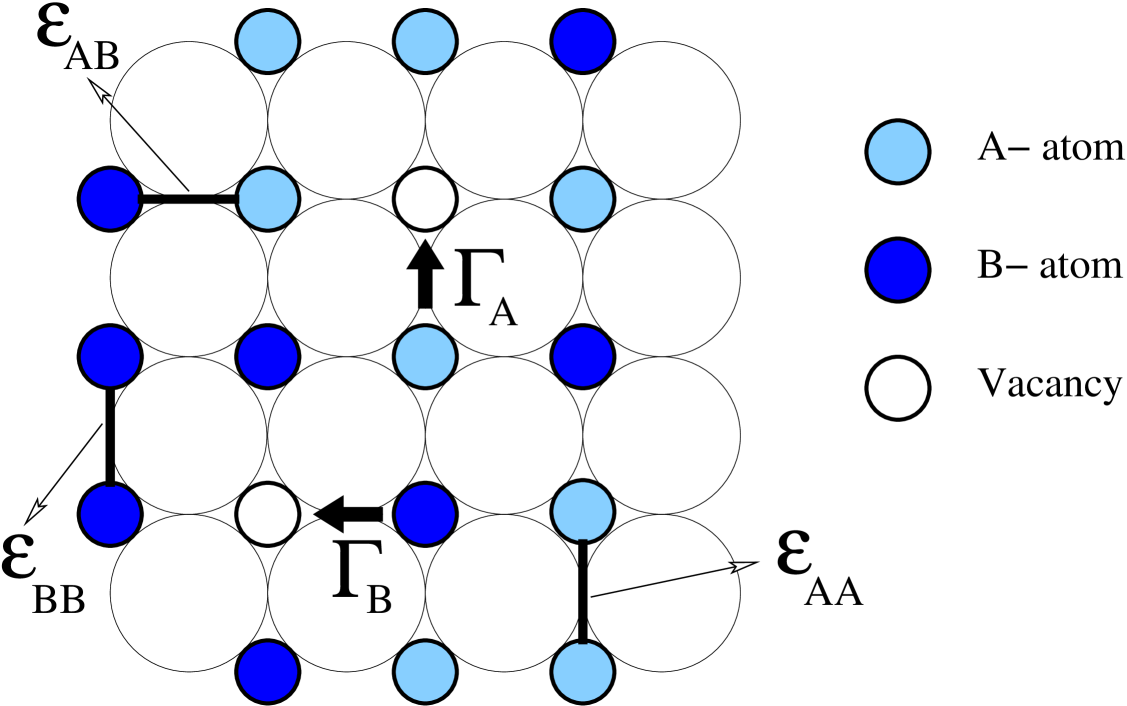
Figure 1: Schematic view of the $(100)$ surface of a substrate (shown as large open circles), whose periodic potential provides a square lattice of prefered adsorption sites (which here are assumed in the center of the square formed by the substrate atoms). $A$-atoms are shown as black circles, $B$-atoms are shown as grey circles, and vacancies ($V$) are shown as empty circles. The energies of the nearest-neighbor interactions between different kind of atoms (indicated by thick lines) are labeled by $\epsilon_{AA}$, $\epsilon_{BB}$ and $\epsilon_{AB}$ respectively. The simple choice $\epsilon_{AB}\equiv\epsilon$, $\epsilon_{AA}=\epsilon_{BB}\equiv 0$ is taken througout. This means that $A-$atoms prefer $B-$atoms as nearest neighbors, but it does not matter whether its nearest neighbors are also $A-$atoms or vacancies, respectively. The jump rates for $A-V$ and $B-V$ exchanges are labeled by $\Gamma_{A}$ and $\Gamma_{B}$, respectively. For simplicity, the $B-$atoms are considered as the faster particles ($\Gamma_{B}\equiv 1$), and $\Gamma_{A}<\Gamma_{B}$.

Having in mind the application of our work to two-dimensional surface alloys, we assume a perfect square lattice of adsorption sites (Fig. 1). These adsorption sites can either be taken by an A-atom, a B-atom, or a vacancy. Therefore this model traditionally is also referred to as the ABV model 17 ; 21 . It can also be viewed as an extension of simple lattice gas models, where diffusion of a single species (A) occurs by hopping to vacant sites, to two components. Diffusion in lattice gases with a single species has been extensively studied 5 ; 22 ; 23 ; 24 ; 25 ; 26 ; 27 ; 28 ; 29 ; 30 , but diffusion in a two-component lattice gas so far has been thoroughly examined only in the noninteracting case 17 . Here we restrict attention to a model with strictly pairwise interactions between nearest neighbors only, which we denote as $\epsilon_{AA},\epsilon_{AB}$ and $\epsilon_{BB}$ pairs. However, in general one can consider also energy parameters between pairs of lattice sites involving one ($\epsilon_{AV}$, $\epsilon_{BV}$) or two ($\epsilon_{VV}$) vacancies, but here we do not consider the $ABV$ model in full generality, but only the special case $\epsilon_{AV}=\epsilon_{BV}=\epsilon_{VV}=0$, although from first principles electronic structure calculations there is evidence that nonzero $\epsilon_{AV},\epsilon_{BV},\epsilon_{VV}$ may occur bes . While all these parameters affect the diffusion behavior of the model, actually only a subset of them controls the static behavior. With respect to static properties of this model, the well-known transcription to the spin$-1$ Blume-Emery-Griffiths model shows (see e.g. ecm ), that for constant concentrations only three interaction parameters would be needed. Note that although there are three concentration variables, $c_{A},c_{B},$ and $c_{V}$, due to the constraint $c_{A}+c_{B}+c_{V}=1$ only two of them are independent. Actually, the physically most interesting case is the limit $c_{V}\rightarrow 0$, since in thermal equilibrium the concentration of vacancies is very small. In the noninteracting case 17 , it was found that many aspects of this limiting behavior $c_{V}\rightarrow 0$ are already reproduced if the vacancy concentration is of the order of a few percent only, e.g. $c_{V}=0.04$, and in fact we shall adopt this choice in the case of the present simulations. Also for the interacting case the limit $c_{V}\rightarrow 0$ greatly simplifies matters, since then, with respect to static properties, we have to consider only a single energy parameter $\epsilon$, defined by

$$\epsilon\equiv\epsilon_{AB}-(\epsilon_{AA}+\epsilon_{BB})/2.$$ (1)

If $\epsilon<0$, the model in thermal equilibrium will exhibit ordering, while for $\epsilon>0$, phase separation occurs 14 ; 15 ; 31 . In the case of a square lattice, the model in the limit $c_{V}\rightarrow 0$ is equivalent to the two-dimensional Ising model, for which some static properties of interest are exactly known 32 ; 33 ; 34 . In particular, for $c_{A}=c_{B}=1/2$ the critical temperature $T_{c}$ is known exactly, namely

$$k_{B}T_{c}^{max}/|\epsilon|=[\ln(1+\sqrt{2})]^{-1}\approx 1.1345.$$ (2)

This is the maximum value of the critical temperature curve $T_{c}(c_{A})$ at which the order-disorder phase transition occurs. According to the well-known Bragg-Williams mean-field approximation, one would rather obtain $k_{B}T_{c}^{MF}/\epsilon=2$ than the result implied by Eq. (2), $k_{B}T_{c}/\epsilon\approx 1.1345$ 35 . Here and in the following, the maximum value $T_{c}(c_{A}=0.5)$ of the pure model without vacancies is simply denoted as $T_{c}$. However, an even more important failure of the mean field theory is the prediction that an order-disorder transition from the disordered phase to a phase with long-range checkerboard order occurs over the entire concentration range, with $T_{c}(c_{A}\rightarrow 0)\rightarrow 0,\;T_{c}(c_{A}\rightarrow 1)\rightarrow 0$, see 35 for a more detailed discussion of mean field theory. As a matter of fact, long range order is only possible for a much more restricted range of concentrations, namely 35 $0.375\leq c_{A}\leq 0.625$ (note that the pairwise character of the interactions implies a symmetry of the phase diagram around the line $c_{A}=1/2$, in the limit $c_{V}\rightarrow 0$ 14 ; 15 ; 31 ).

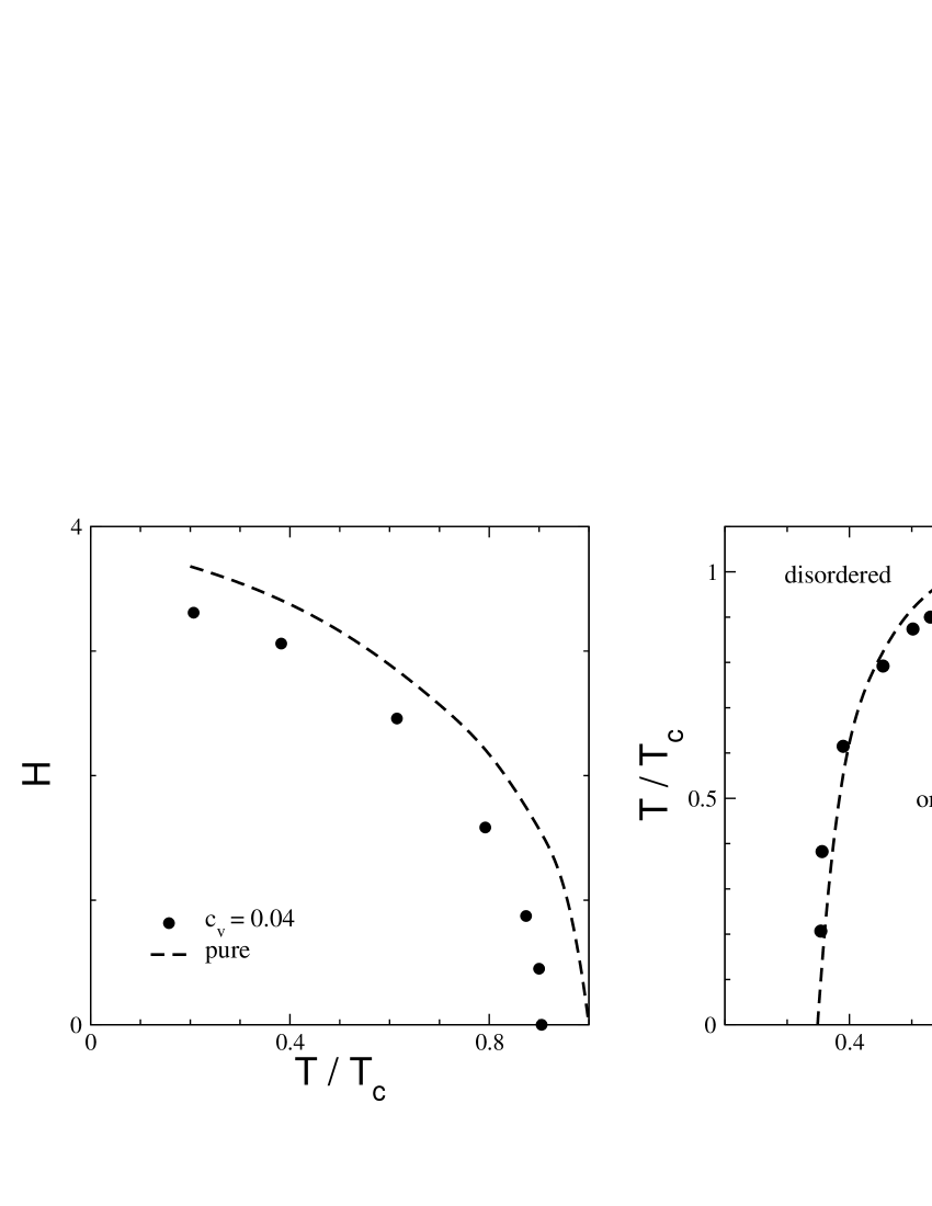
Figure 2: ($a$) Phase boundary for the order-disorder transition of the $ABV$ model with $c_{V}=0.04$. The phase boundary of the pure Ising antiferromagnet 35 (equivalent to the case $c_{V}=0$) is also included for comparison, as a dashed line. ($b$) Critical curve $T$ vs. $c_{A}$, where $c_{A}=1-c_{V}-c_{B}$. The critical curve of the pure Ising antiferromagnet 35 is also included for comparison, as a dashed line. Temperature $T$ is always measured in units of the maximal critical temperature $T_{c}$ of the pure model (no vacancies, $c_{V}=0$ and $c_{A}=c_{B}=0.5)$, cf. text.

If we work with a small but nonzero concentration of vacancies $c_{V}$, the maximum critical temperature no longer occurs at $c_{A}=c_{B}=1/2$, but rather at $c^{*}=c_{A}=c_{B}=(1-c_{V})/2$, and the phase diagram is in this case symmetric around this concentration $c^{*}$. Apart from this statement, there are no longer any exact results available, but it is fairly straightforward to obtain the phase diagram from standard Monte Carlo methods 19 with an accuracy that is sufficient for our purposes. Fig.2 shows our estimates of the phase boundary for $c_{V}=0.04$, in comparison with previous results for $c_{V}=0$. As has been well documented in the literature 19 ; 31 ; 35 , such phase diagrams are conveniently mapped out by transforming the model to a magnetic Ising spin model (representing the cases that lattice site $i$ is taken by an $A-$atom by spin up, $B-$atom by spin down, respectively) and considering the transition from the paramagnetic to the antiferromagnetic phase for various magnetic fields $H$ ($2\;H=\mu_{A}-\mu_{B}$, if $\epsilon_{AA}=\epsilon_{BB}$, and with $\mu_{A}$ and $\mu_{B}$ being the chemical potentials of $A$ and $B-$ particles, respectively). Estimating then the magnetization $m_{c}(H)=m(H,T=T_{c}(H))$ at the phase boundary, one then obtains the corresponding critical concentrations from

$$c^{crit}_{A}(T)=(1\pm m_{c}(T)-c_{V})/2$$ (3)

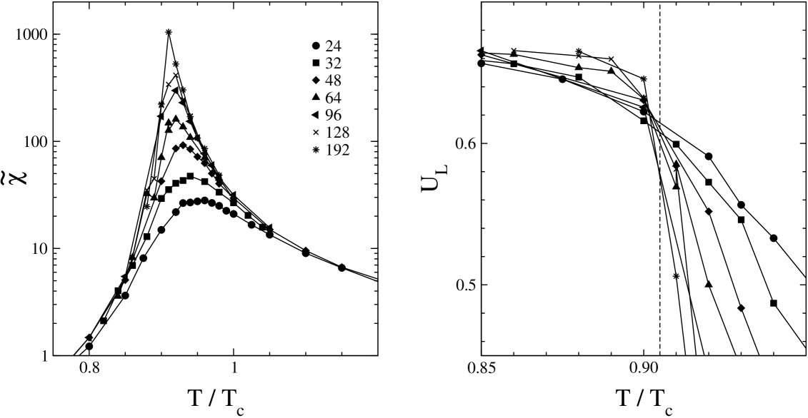
Figure 3: Dependence of the staggered susceptibility $\tilde{\chi}$ ($a$) and the fourth order cumulant $U_{L}$ ($b$) on the temperature, along the critical line $H=0$ corresponding to the critical concentration $c_{A}=0.48$. Several system sizes are considered, as indicated. Here $T_{c}$ denotes the maximal critical temperature of the model without vacancies ($H=0$ then corresponds to $c_{A}=0.5$).

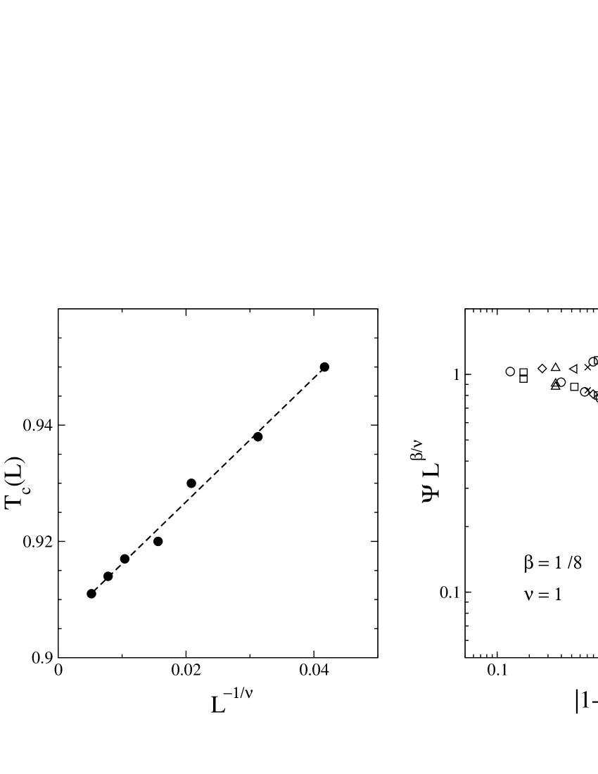
Figure 4: ($a$) Plot of the size-dependent critical temperature $T_{c}(L)$ (defined as the maximum of $\tilde{\chi}(T,L)$), in terms of the scaled variable $L^{1/\nu}$. The critical Ising exponent $\nu=1$ is employed. The linear extrapolation to the thermodynamic limit, shown as a dashed line, provides an estimation of $T_{c}(c_{V}=0.04)=0.905(5)$ for the $ABV$ model with $c_{V}=0.04$. ($b$) Scaling plot of the order parameter $\psi$. The estimated critical temperature and the Ising critical exponents $\nu=1$ and $\beta=1/8$ are employed.

Fig. 2 shows that for $c_{V}=0.04$ the maximum critical temperature occurs for $T_{c}(c_{V}=0.04)/T_{c}\approx 0.905$, and for $T\rightarrow 0$ the phase boundary ends at the concentrations $c_{A,1}^{crit}\approx 0.375,\;c_{A,2}^{crit}\approx 0.585$. As it should be, the phase diagram is symmetric around $c_{A,max}^{crit}=(1-c_{V})/2=0.48$. The analysis indicates that the order-disorder transition stays second order throughout, also in the presence of this small vacancy concentration. Although it is clear that a vacancy concentration of $c_{V}=0.04$ does have some clearly visible effects, in comparison to the model with $c_{V}\rightarrow 0$, these changes do not affect the qualitative character of the phase behavior, but cause only minor modifications of quantitative details. For obtaining accurate results on the dynamic behavior of the model with a modest amount of computing time, working with sufficiently many vacancies on the lattice is mandatory. Note that for the diffusion studies we use a lattice of linear dimensions $L=1024$, while the static phase diagram was extracted from a standard finite size scaling analysis 19 , see Figs. 3, 4 for an example, using sizes $24\leq L\leq 192$. Periodic boundary conditions are applied throughout. The static quantities that were analyzed in order to obtain the phase boundary are the antiferromagnetic order parameter $\Psi$ (we refer here to the transformation of the model to the Ising spin representation again)

$$\Psi=\langle|\phi|\rangle,\;\;\;\phi=L^{-2}\sum\limits^{L}_{k=1}\sum\limits_{\ell=1}^{L}(-1)^{k+\ell}S_{k,\ell}\,\,,$$ (4)

where $k,\ell$ label the lattice sites in $x-$ and $y-$ direction, respectively. Similarly, the magnetization $m$ is given by averaging all the spins without a phase factor

$$m=\langle M\rangle,\quad M=L^{-2}\sum\limits_{k=1}^{L}\sum\limits_{\ell=1}^{L}S_{k,\ell}\,\,,$$ (5)

and the susceptibility $\chi$ and staggered susceptibility $\tilde{\chi}$ are obtained from the standard fluctuation relations

$$\chi=L^{2}(\langle M^{2}\rangle-\langle M\rangle^{2})/k_{B}T\;,$$ (6)

$$\tilde{\chi}=L^{2}(\langle\phi^{2}\rangle-\langle|\phi|\rangle^{2})/k_{B}T\,\,.$$ (7)

Note that in a finite system in the absence of symetry-breaking fields one needs to work with the average of the absolute value $\langle|\phi|\rangle$ rather than $\langle\phi\rangle$ in order to have a meaningful order parameter 19 .

A further quantity useful for finding the location of the transition is the fourth order cumulant of the order parameter 36

$$U_{L}=1-\langle\phi^{4}\rangle/[3\langle\phi^{2}\rangle^{2}]\,,$$ (8)

since the critical temperature can be found from the intersection of the cumulants plotted versus temperature for different lattice sizes. For the two-dimensional Ising universality class, this intersection should occur for a value $U^{*}\approx 0.6107$ 37 .

Fig. 3 shows that this expectation is only rather roughly fulfilled. To some extent this may be attributed to statistical errors, but in addition probably for $c_{V}\neq 0$ there are somewhat larger corrections to finite size scaling than for the “pure” model (i.e., the model without vacancies). We have hence estimated $T_{c}(c_{V}=0.04)$ alternatively from a plot of the temperatures $T_{c}(L)$, where the maximum of $\tilde{\chi}(T,L)$ for finite $L$ occurs, versus the finite size scaling variable $L^{-1/\nu}=L^{-1}$ (remember $\nu=1$ in the two-dimensional Ising model 34 ), see Fig. 4a. The quality of the finite size scaling “data collapse” of the order parameter (fig. 4b) gives us confidence in the reliability of our procedures.

We emphasize that the present paper concerns only the choice of the symmetric case, $\epsilon_{AA}=\epsilon_{BB}$. While any asymmetry between $A$ and $B$, leading to $\epsilon_{AA}\neq\epsilon_{BB}$, has little effect on static properties for small $c_{V}$, the distribution of the vacancies and their dynamics may get strongly affected by such an asymmetry ecm ; 21 .

Finally, we mention a static quantity that plays a role in discussing the self-diffusion coefficient of particles in lattice gas models, the so-called “vacancy availability factor” 5 ; 23 ; 29

$$V=c_{V}(1-\alpha_{1})$$ (9)

Here $\alpha_{1}$ is the standard Cowley-Warren short range order parameter 14 ; 15 ; 16 ; 31 for the nearest neighbor shell of a particle: $\alpha_{1}=0$ if there is a random occupation of the lattice sites by any particles and vacancies (note that here we are not concerned with short range order describing the non-random occupation of $A$ versus $B$ particles on the lattice. Due to the symmetry $\epsilon_{AA}=\epsilon_{BB}$, there is also no need to consider separate vacancy availability factors for $A$ and $B$ particles). Actually, we expect that in the limit $c_{V}\rightarrow 0$ also $\alpha_{1}\rightarrow 0$, and then $V=c_{V}$. Hence a calculation of $\alpha_{1}$ can serve as a test whether the chosen vacancy concentration is small enough in order to reproduce the desired limit $c_{V}\rightarrow 0$.

III SIMULATION METHODOLOGY TO STUDY TRANSPORT PHENOMENA

The Monte Carlo simulations consist of an initial part, necessary to equilibrate the system for the desired conditions, and a final part, where the transport coefficients of interest are “measured” in the simulation. While in the case of the completely random $ABV$ alloy studied in 17 the generation of an initial configuration is straightforward, this is not so here, because depending on where the chosen state point $(T,c_{A})$ is in the phase diagram, Fig. 2, we have long range order or not. If the system in equilibrium is in a state where long range order occurs, it is important to prepare the system in a monodomain sample: otherwise the presence of antiphase domain boundaries 31 might spoil the results. In particular, at very low temperature interdiffusion could be strongly enhanced near such boundaries, in comparison with the bulk. Although such effects are interesting in their own right, they need separate study from bulk behavior, and are out of consideration here.

Actually the best way to prepare the equilibrated initial configurations, in cases where long range order is present, is the use of the “magnetic” representation of the model as an Ising antiferromagnet in a field $H$ (remember that $H$ physically corresponds to the chemical potential difference between $A$ and $B$ particles 31 ). Recording the magnetization $m(T,H)$ as function of the field, one can choose the field such that states with the desired value of $m$ and hence $c_{A}=(1-c_{V}-m)/2$ result. The initial spin configuration is that of a perfect antiferromagnetic structure, from which a fraction $c_{V}$ of sites chosen at random is removed. The Monte Carlo algorithm that was used is the standard single spin flip Metropolis algorithm 19 , mixed with random exchanges of the vacancies with randomly chosen neighbors. Note that during this equilibration part the concentration $c_{A}$ is not strictly constant, but slightly fluctuating: this lack of conservation of $c_{A}$ is desirable, however, since “hydrodynamic slowing down” 19 of long wavelength concentration fluctuations would otherwise hamper the equilibration of concentration correlations at long distances.

In the final stage of the Monte Carlo runs, of course, the spin flip Monte Carlo moves are shut off, since for the analysis of the diffusion constants the concentrations $c_{A},c_{B}=1-c_{V}-c_{A}$ need to be strictly conserved. Most straightforward is the estimation of the self-diffusion coefficients (also called “‘tracer diffusion coefficients”) $D_{t}$ of tagged $A$ and $B$ particles, since there one simply can apply the Einstein relation

$$\langle r^{2}\rangle=2\,d\,D_{t}\,t,\;\;\;\;\;\;t\rightarrow\infty,\;\;\;\;\;\;r=\vec{r}_{i}(t)-\vec{r}_{i}(0),$$ (10)

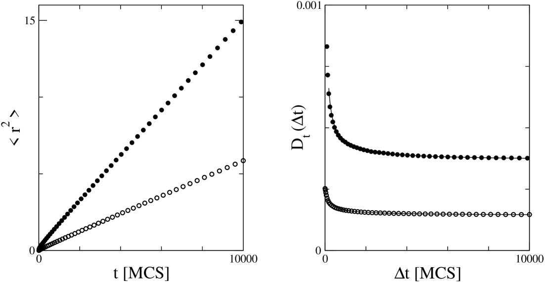
Figure 5: Determination of the tracer diffusion coefficients. ($a$) Mean square displacements of tagged $A$ particles (open dots) and $B$ particles (full dots) as a function of Monte Carlo steps per particle. The temperature is $T=1.2$ (in units of the Ising critical temperature), and the concentrations are $c_{A}=0.4$, $c_{B}=0.56$. The ratio of jump rates is $\Gamma_{A}/\Gamma_{B}=0.01$. ($b$) Estimates of the tracer diffusion coefficients as a function of the time interval used. The lines represent the fits of the data after using Eq. (11).

$d$ being the dimensionality of the lattice ($d=2$ here), and $\vec{r}_{i}(t)$ being the position of the $i$-th particle at time $t$. Fig. 5 illustrates the application of this method for a typical example, in the case $\Gamma_{A}/\Gamma_{B}=0.01$, temperature $T=1.2$ (in units of $T_{c}$, Eq. 2), and concentrations $c_{A}=0.40,c_{B}=0.56$, respectively. While the plot of $\langle r^{2}\rangle$ vs. $t$, for a total time of $t=10^{4}$ MCS, look at first sight almost linear (Fig. 5, left part), a closer look reveals a slight but systematic decrease of the slope of the $\langle r^{2}\rangle$ vs. $t$ curve with increasing time. A similar observation was already reported by Kehr et al. 17 , who attributed this decrease of slope to the presence of a logarithmic correction.

Specifically, it was shown that in $d=2$ the estimate $D_{est}(\Delta t)$ of the tracer diffusion constants depend on the time interval $\Delta t$ of estimation as

$$D_{est}(\Delta t)=A+B\ln(\Delta t)/\Delta t+C/\Delta t\;,$$ (11)

where $A,B,C$ are phenomenological constants. Therefore we have analyzed $D_{est}(\Delta t)$ as a function of $\Delta t$ in the present case (Fig. 5, right part). We found rather generally that there is a significant dependence of $D_{est}(\Delta t)$ on $\Delta t$ for $\Delta t\leq 2.10^{3}$, while for $\Delta t\geq 5.10^{3}$ the dependence on $\Delta t$ can safely be neglected. A remarkable feature of the results also is that the faster B particles exhibit (in the example shown in Fig. 5) a diffusion constant that is only about a factor of three larger than the slower A particles, while the jump rate is a factor of 100 larger. This fact already indicates that there is no straightforward relation between the tracer diffusion constants and the jump rates.

In the description of collective diffusion, the Onsager coefficients $\Lambda_{AA}$, $\Lambda_{AB}$, $\Lambda_{BA}$ and $\Lambda_{BB}$ play a central role, since they appear as coefficients in the linear relations between particle currents $\vec{j}_{A},\vec{j}_{B}$ and the corresponding driving forces, the gradients of the potential differences between A (or B) particles and vacancies V, respectively 17 :

$$\vec{j}_{A}=-(\Lambda_{AA}/k_{B}T)\nabla(\mu_{A}-\mu_{V})-(\Lambda_{AB}/k_{B}T)\nabla(\mu_{B}-\mu_{V}),$$ (12)

$$\vec{j}_{B}=-(\Lambda_{BA}/k_{B}T)\nabla(\mu_{A}-\mu_{V})-(\Lambda_{BB}/k_{B}T)\nabla(\mu_{B}-\mu_{V})\;.$$ (13)

Note that due to the symmetry relation

$$\Lambda_{BA}=\Lambda_{AB}$$ (14)

only three of these four Onsager coefficients are thought to be independent. There is no simple relation between the two jump rates $\Gamma_{A},\Gamma_{B}$ (and temperature T and the concentrations $c_{A},c_{B}$) and these three Onsager coefficients $\Lambda_{AA},\Lambda_{AB},\Lambda_{BB}$, of course. Hence it is a task of the simulation to estimate these Onsager coefficients, and it is well known 17 ; 22 that this can be done by applying a force to the particles, which acts in the same way as a chemical potential gradient. Due to the periodic boundary conditions, particles that leave the box at one side will reenter at the opposite one, and hence a chemical potential gradient causes a steady state flux of particles through the simulation box in the direction of this driving force. Care is needed in two respects:

• One must average long enough to make sure that slow transients after the imposition of the force have died out and steady-state conditions are actually reached.

• One must make sure that the applied force is small enough so one works in the region where the response of the system to this force is strictly linear, as written in Eqs. (12), (13), and nonlinear corrections can be completely neglected.

This method of estimating Onsager coefficients was pioneered by Murch and Thorn 22 for one-component lattice gases and extended to random alloy models in 17 ; 38 . We refer the reader to these papers for a more detailed justification and discussion of this method. Following 17 we implement this force on species of particles $\gamma$ ($\gamma=A$ or $B$) by taking the jump rates in the $x-$ direction as

$$\Gamma_{x}^{(\gamma)}=b\,\Gamma_{\gamma},\;\;\Gamma_{-x}^{(\gamma)}=b^{-1}\,\Gamma_{\gamma},\;\;b>1$$ (15)

while the jump rate in the $\pm y-$ directions remains $\Gamma_{\gamma}$. If we would have a single particle (s.p.) only, the mean velocity in the $+x-$ direction would be $v_{x}^{s.p.}=\Gamma_{\gamma}(b-b^{-1})$, which should correspond to $v_{x}^{s.p.}=(\Gamma_{\gamma}/k_{B}T)F_{x}$, $F_{x}$ being the force in $x-$ direction, in the regime of linear response. Hence one concludes that from the velocity of species $\alpha$ one can deduce the Onsager coefficient $\Lambda_{\alpha\gamma}$ if a force $F_{x}$ is exerted on species $\gamma$ via

$$v_{x}^{(\alpha)}/v^{s.p.}_{x}=(\Gamma_{\alpha}c_{\alpha})^{-1}\Lambda_{\alpha\gamma}.$$ (16)

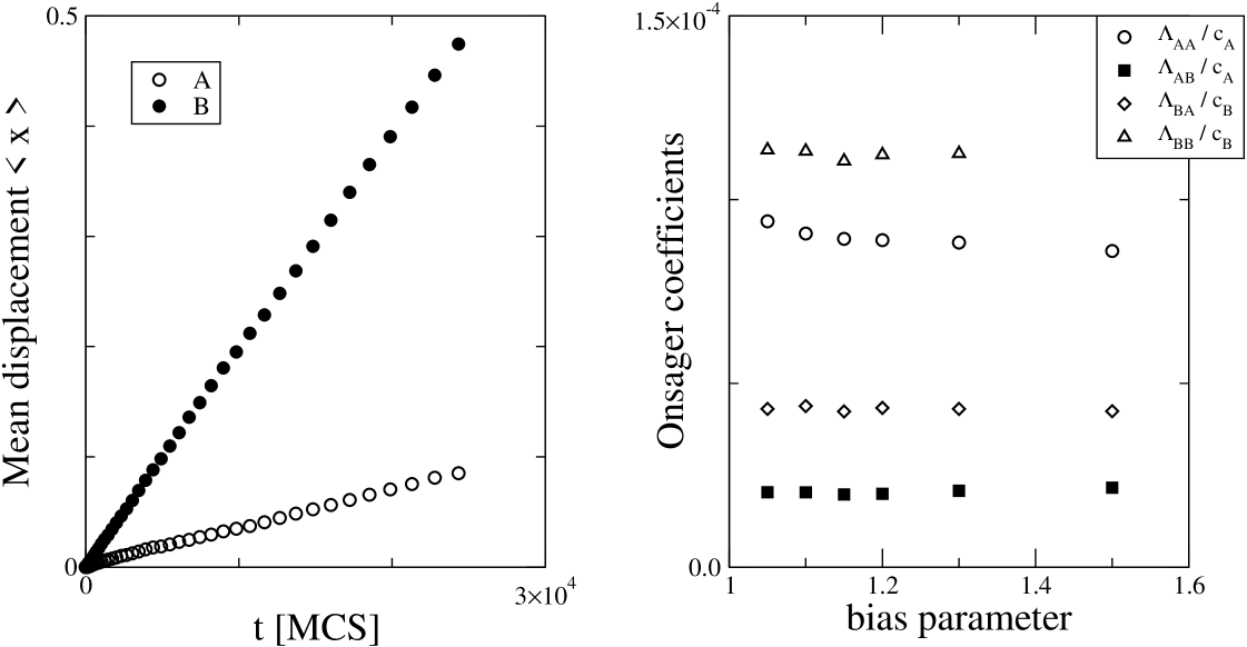
Figure 6: Determination of the Onsager coefficients. ($a$) Mean displacements along the $x-$ direction of $A$ and $B$ particles as a function of Monte Carlo steps per particle. The temperature is $T=0.6$, and the concentrations are $c_{A}=0.71$, $c_{B}=0.25$. The ratio of jump rates is $\Gamma_{A}/\Gamma_{B}=0.01$, and the bias parameter is $b=1.1$. ($b$) Estimates of the Onsager coefficients $\Lambda_{ij}/c_{i}$ by extrapolation to bias parameter $b=1$.

The application of this method is illustrated in Fig. 6. There the mean displacement $\langle x\rangle$ of $A-$ and $B-$ particles is followed over $2.5\times 10^{4}$ Monte Carlo steps (MCS) per site, and a very good linearity of $\langle x\rangle$ vs. $t$ is observed (left part). In order to check for nonlinear effects, the bias parameter $b$ is varied in the range $1.05\leq b\leq 1.5$, and the results are extrapolated to $b\rightarrow 1$. (right part of Fig. 6). Consistent with previous work on the random $ABV$ model 17 , nonlinear effects are rather weak, and in this way we are able to estimate Onsager coefficients with a relative error of a few percent.

Still a different approach was followed to estimate the interdiffusion constant $D_{int}$. We prepare a system in thermal equilibrium in the presence of a wavevector-dependent chemical potential difference $\delta\mu(x)$ defined as

$$\delta\mu(x)\equiv\mu_{A}(x)-\mu_{B}(x)\equiv\hat{\delta}\cos(\frac{2\pi}{\lambda}x),$$ (17)

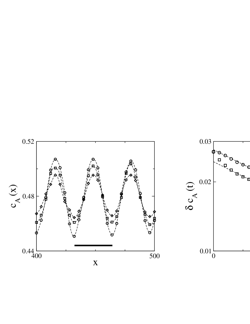
Figure 7: Determination of the interdiffusion coefficients. For $t<0$ we impose a cosine-like varying bulk field $H(x)$ which introduces a modulation in the concentration of $A$ and $B$ particles. The characteristic length of this perturbation is $\lambda=32$ lattice spacings. ($a$) Temporal evolution of the concentration of $A$ particles along the $x-$ direction in the lattice. Times correspond to $t=0$ (circles), $t=10000$ (squares) and $t=20000$ (diamonds), respectively. The thick line marks the wavelenght $\lambda=32$ of the applied bulk field. The temperature is $T=1.5$, and the concentrations are $c_{A}=c_{B}=0.48$. The ratio of jump rates is $\Gamma_{A}/\Gamma_{B}=0.01$. ($b$) Amplitude of concentration profiles as a function of time, for $A$ particles (circles) and $B$ particles (squares). The dashed lines correspond to fits of the data to single exponential functions, characterized by a decay constant $D_{int}$.

$\hat{\delta}$ being an amplitude that needs to be chosen such that the resulting concentration variation is still in the regime where linear response holds, and $\lambda$ is the wavelength of the modulation (which is chosen such that the linear dimension $L$ of the lattice is an integer multiple of $\lambda$). Note that in the Ising spin representation $\delta\mu(x)$ simply translates in a wavelength-dependent magnetic field, of course. The system then is equilibrated in the presence of this perturbation for a large number of Monte Carlo steps (of the order of $10^{6}$ MCS). This causes a corresponding periodic concentration variation, see Fig. 7, left part. The sinusoidal shape of this initial concentration variation provides a confirmation that the linear response description is applicable otherwise the presence of higher harmonics in the concentration variation would indicate the presence of nonlinear effects. Then a “clock” is set to time $t=0$ and the perturbation $\delta\mu(x)$ is put to zero for times $t>0$. As a consequence, the concentration variation decays to zero as the time $t\rightarrow\infty$. It turns out that this decay with time can be described by a superposition of two simple exponential decays, one governing the decay of the concentration difference $\delta c(x)=c_{A}(x)-c_{B}(x)$ of the particles, the other corresponding to the decay of the total density. As discussed in detail for the random $ABV$ model 17 , the concentration variation can be described therefore as ($k=2\pi/\lambda$, and $D_{+}>D_{-}$ are two diffusion constants)

$$\delta c_{A}(t)=\hat{c}_{A}^{+}\exp(-D_{+}k^{2}t)+\hat{c}_{A}^{-}\exp(-D_{-}k^{2}t)\;,$$ (18)

$$\delta c_{B}(t)=\hat{c}_{B}^{+}\exp(-D_{+}k^{2}t)+\hat{c}_{B}^{-}\exp(-D_{-}k^{2}t)\;,$$ (19)

where $\hat{c}_{A}^{+},\hat{c}_{A}^{-},\hat{c}_{B}^{+},\hat{c}_{B}^{-}$ are amplitude prefactors, which one can estimate from the treatment that will be outlined in the following section. Here we only mention that $\hat{c}_{A}^{+}+\hat{c}_{A}^{-}=\delta c_{A}(0),\;\hat{c}_{B}^{+}+\hat{c}_{B}^{-}=\delta c_{B}(0)$, and in the limit $c_{V}\rightarrow 0$ we have $\hat{c}_{A}^{+},\hat{c}_{B}^{+}\propto c_{V}\rightarrow 0$, while $\hat{c}_{A}^{-},\hat{c}_{B}^{-}$ stay finite (of the order of $\hat{\delta}$). In this limit the two diffusion constants $D_{+},D_{-}$ are of very different order of magnitude, since $D_{-}\propto c_{V}$, while $D_{+}$ stays of order unity 17 . Thus density variations have a very small amplitude (of order $c_{V}$) and decay fast, while concentration variations decay much slower. This consideration leads us to identify $D_{-}$ as the interdiffusion constant $D_{int}$ in this limit. For finite nonzero $c_{V}$, however, in principle both density and concentration variations are coupled, and both diffusion constants $D_{+},D_{-}$ contribute to the interdiffusion of $A$ and $B$ particles 17 .

The right part of Fig. 7 illustrates that even for $c_{V}$ as large as $c_{V}=0.04$ there is already a reasonable separation between density and concentration fluctuations: both $\delta c_{A}(t)$ and $\delta c_{B}(t)$ reach their asymptotic decay (where only the same factor $\exp(-D_{-}k^{2}t)$ matters, as is evident from the fact that there are two parallel straight lines on the semilog plot) already at a time $t\approx 2000$, long before the concentration variations have decayed to zero.

IV THEORETICAL PREDICTIONS

A basic ingredient of all analytical theories are the conservation laws for the numbers of A and B particles, which lead to continuity equations for the local concentrations $c_{A}(\vec{r},t),c_{B}(\vec{r},t)$

$$\frac{\partial c_{A}(\vec{r},t)}{\partial t}+\nabla\cdot\vec{j}_{A}(\vec{r},t)=0,$$ (20)

$$\frac{\partial c_{B}(\vec{r},t)}{\partial t}+\nabla\cdot\vec{j}_{B}(\vec{r},t)=0,$$ (21)

Note that these equations hold rigorously, if a local concentration field $c_{\alpha}(\vec{r},t)$ $\{\alpha=A,B\}$ can be defined, unlike the so-called constitutive relations, Eqs. (12),(13), which are only approximately true: these equations only are supposed to hold in the case that the gradients $\nabla(\mu_{A}-\mu_{V}),\nabla(\mu_{B}-\mu_{V})$ are sufficiently small, otherwise the relation between currents and gradients is non linear. In addition, a second requirement is that statistical fluctuations can be neglected; otherwise a random force term needs to be added on the right hand side of Eqs. (12),(13) 39 . We also note that in our model (unlike real alloys, where vacancies can be created by hopping of atoms from lattice sites to interstitial sites, and where vacancies can be destroyed by hopping of interstitial atoms to a neighboring vacant site of the lattice 1 ; 2 ; 3 ) also vacancies are conserved, and hence

$$\frac{\partial c_{V}(\vec{r},t)}{\partial t}+\nabla\cdot\vec{j}_{V}(\vec{r},t)=0.$$ (22)

However, as discussed in 17 there is no need to include $c_{V}(\vec{r},t)$ and $\vec{j}_{V}(\vec{r},t)$ as additional dynamical variables in the problem: the condition that every lattice site is either occupied by an A-atom, B-atom or vacant (V) translates into the constraint $c_{A}(\vec{r},t)+c_{B}(\vec{r},t)+c_{V}(\vec{r},t)=1$. Similarly, one finds that $\vec{j}_{V}=-(\vec{j}_{A}+\vec{j}_{B})$ 17 .

In order to be able to relate the chemical potentials in Eqs. (12),(13) to the concentration variables, we use the thermodynamic relation

$$\mu_{\alpha}=\left(\frac{\partial F}{\partial N_{\alpha}}\right)_{{T,N}_{\beta(\neq\alpha)}}\;,$$ (23)

$N_{\alpha}$ being the number of particles of species $\alpha$, and $F$ being the total free energy of the system. We decompose $F$ into the internal energy $U$ and the entropic contribution $-TS$, with $S$ being simply the entropy of mixing

$$S=-k_{B}[N_{A}\ln N_{A}+N_{B}\ln N_{B}+N_{V}\ln N_{V}-N\ln N]\;,$$ (24)

where $N=N_{A}+N_{B}+N_{V}$ then is the total number of sites on the lattice, and $c_{\alpha}=N_{\alpha}/N$ then is the concentration of species $\alpha$. While Eq. (24) is exact in the non-interacting $ABV$ model, it still holds in the disordered phase of the interacting model in the framework of the Bragg-Williams mean field approximation. In the disordered phase, no sublattices need to be introduced, and then the concentration variables on average are the same for all lattice sites. Then $U$ can be written as

$$U=\frac{1}{2}Nz(\epsilon_{AA}c_{A}^{2}+2\epsilon_{AB}c_{A}c_{B}+\epsilon_{BB}c^{2}_{B}),$$ (25)

where $z$ is the coordination number of the lattice, and consistent with the simulated model (Sec.II) a nearest neighbor interaction is assumed. Note that the basic approximation of Eq. (25) is the neglect of any correlation in the occupancy of neighboring lattice sites.

With some algebra 17 one can reduce Eqs. (12), (13), (20)-(25) to a set of two coupled diffusion equations

$$\frac{\partial c_{\alpha}}{\partial t}=\sum\limits_{\beta}D_{\alpha\beta}\nabla^{2}c_{\beta}\;,$$ (26)

where the elements $D_{\alpha\beta}$ of the diffusion matrix are given by

$$D_{AA}=\Lambda_{AA}(\frac{1}{c_{A}}+\frac{1}{c_{V}}+\frac{z\epsilon_{AA}}{k_{B}T})+\Lambda_{AB}(\frac{1}{c_{V}}+\frac{z\epsilon_{AB}}{k_{B}T})\;,$$ (27)

$$D_{AB}=\Lambda_{AA}(\frac{1}{c_{V}}+\frac{z\epsilon_{AB}}{k_{B}T})+\Lambda_{AB}(\frac{1}{c_{B}}+\frac{1}{c_{V}}+\frac{z\epsilon_{AA}}{k_{B}T})\;,$$ (28)

$$D_{BA}=\Lambda_{AB}(\frac{1}{c_{A}}+\frac{1}{c_{V}}+\frac{z\epsilon_{AA}}{k_{B}T})+\Lambda_{BB}(\frac{1}{c_{V}}+\frac{z\epsilon_{AB}}{k_{B}T})\;,$$ (29)

$$D_{BB}=\Lambda_{AB}(\frac{1}{c_{V}}+\frac{z\epsilon_{AB}}{k_{B}T})+\Lambda_{BB}(\frac{1}{c_{B}}+\frac{1}{c_{V}}+\frac{z\epsilon_{BB}}{k_{B}T})\;.$$ (30)

Note that $D_{AB}\neq D_{BA}$. Introducing Fourier transforms and diagonalizing the diffusion matrix the solution indeed can be cast into the form of Eqs. (18),(19). As has already been mentioned in this context, for $c_{V}\rightarrow 0$ the two eigenvalues $D_{+},D_{-}$ of the diffusion matrix adopt very different orders of magnitude 17 :

$$D_{+}\approx(\Lambda_{AA}+2\Lambda_{AB}+\Lambda_{BB})/c_{V},$$ (31)

$$D_{-}\approx\frac{\Lambda_{AA}\Lambda_{BB}-\Lambda^{2}_{AB}}{\Lambda_{AA}+2\Lambda_{AB}+\Lambda_{BB}}(\frac{1}{c_{A}}+\frac{1}{c_{B}}-\frac{2z\epsilon}{k_{B}T}).$$ (32)

Since in this limit the $\Lambda_{\alpha\beta}\propto c_{V}$, the coefficient $D_{+}$ reaches a finite limit for $c_{V}\rightarrow 0$, while $D_{-}\propto c_{V}$. We also recognize that $D_{-}$ can be decomposed into a product of two factors: a “kinetic factor” $\Lambda_{int}$, composed by a combination of Onsager coefficients, and a “thermodynamic factor”, which is nothing but an effective inverse “susceptibility” $\chi^{-1}$ describing concentration fluctuations, normalized per lattice site,

$$\chi^{-1}=c_{A}^{-1}+c_{B}^{-1}-2z\epsilon/k_{B}T=[c_{A}(1-c_{A})]^{-1}-2z\epsilon/k_{B}T$$ (33)

In the last step, we used the fact that $c_{B}=1-c_{A}$ for $c_{V}\rightarrow 0$. We call $\chi$ a “susceptibility” because in the translation to the Ising spin representation $\chi$ simply becomes proportional to the derivative of the “magnetization” with respect to the field. Note that for $\epsilon>0$ (i.e., a mixture with unmixing tendency) Eq. (33) exhibits a vanishing of $\chi^{-1}$ and hence of the interdiffusion constant $D_{-}$ at the mean field spinodal curve, defined by

$$k_{B}T_{s}(c_{A})/\epsilon=2c_{A}(1-c_{A})z\;.$$ (34)

The mean field spinodal touches the coexistence curve of such a phase-separating mixture at its maximum in the critical temperature, i.e. $k_{B}T_{c}^{MF}/\epsilon=z/2=2$, for a square lattice. Actually, the symmetry of the Ising Hamiltonian in zero field implies that the maximum critical temperature of the Ising antiferromagnet, which occurs at zero field as well, then is also given by

$$k_{B}\,T_{\,c,max}^{\,MF}/|\epsilon|=z/2=2,\quad\epsilon<0$$ (35)

Comparing this estimate to the exact result, Eq.( 2), we notice that the mean field approximation actually overestimates the maximum critical temperature of the ordering alloy by almost a factor of two, as is well known. Note that this error increases for $c_{A}\neq 1/2$ 35 . So Eq. (32) cannot be assumed to be quantitatively reliable. Note that for ordering alloys (where $\epsilon<0$) the interdiffusion constants gets enhanced (rather than reduced, as it happens for alloys with unmixing tendency) as an effect of the interactions. Beside that, Eq. (32) does not predict any singularity of $D_{-}$ as one approaches the order-disorder phase boundary $T_{c}(c_{A})$ from the disordered side.

Discussing now the kinetic factor $\Lambda_{int}$, we recall the popular approximation to neglect the off-diagonal Onsager coefficient in comparison to the diagonal ones. This leads to

$$\Lambda_{int}\approx\Lambda_{AA}^{-1}+\Lambda_{BB}^{-1}$$ (36)

With this approximation, Eq. (32) reduces to the well-known “slow mode theory ” of interdiffusion, which has been much debated in the case of fluid polymer mixtures 40 -45 . A mean field type approximation for self-diffusion 17 ; 40 ; 41 ; 42 ; 43 then relates the Onsager coefficients $\Lambda_{AA},\Lambda_{BB}$ and tracer diffusion coefficients $D_{t}^{A},D_{t}^{B}$,

$$\Lambda_{AA}=D_{t}^{A}c_{A}\;,\quad\Lambda_{BB}=D_{t}^{B}c_{B}$$ (37)

and thus the “slow mode” theory predicts the following relation between tracer diffusion coefficients and the interdiffusion constant (remember $c_{B}=1-c_{A}$ for $c_{V}\rightarrow 0$)

$$D_{int}^{s.m.}=\{(D_{t}^{A}c_{A})^{-1}+[D_{t}^{B}(1-c_{A})]^{-1}\}\{[c_{A}(1-c_{A})]^{-1}-2z\epsilon/k_{B}T\}.$$ (38)

A rather different result, the so-called “fast mode” theory 44 ; 45 , can be obtained by several distinct arguments. We mention only one of these arguments here, which starts from the assumption 44 that everywhere the vacancy concentration $c_{V}(\vec{r},t)$ is in thermal equilibrium, i.e.

$$\nabla\mu_{v}=0.$$ (39)

Of course, in our model Eq. (39) cannot be justified, in view of the constraints $c_{V}(\vec{r},t)=1-c_{A}(\vec{r},t)-c_{B}(\vec{r},t)$, $\vec{j}_{V}=-(\vec{j}_{A}+\vec{j}_{B})$ and Eqs. (22)-(24) there is no freedom to make additional assumptions on $\mu_{V}$ at all, $\nabla\mu_{V}(\vec{r},t)$ already is determined from these other equations. However, the motivation for Eq. (39) is that for real systems there is no strict conservation for the number of vacancies: in real (three-dimensional) alloys, vacancies can be created and destroyed by formation or annihilation of interstitial atoms, or by interaction with other lattice imperfections such as dislocations, grain boundaries, etc. For two-dimensional surface alloys 20 , vacancies can be created and destroyed if an atom from the considered surface monolayer becomes an adatom on top of this monolayer, or an adatom executing surface diffusion 18 ; 30 becomes incorporated into the monolayer via a jump to a vacant site inside the monolayer. In view of these physical mechanisms which are forbidden in our model, Eq. (39) may represent a physically interesting limiting case. A priori, it is not clear for a particular system, whether for the time scales of interest it is closer to a situation where vacancies are in equilibirum (Eq. (39)) or conserved (Eq. (22)). Our numerical studies are concerned with the latter case exclusively. Nevertheless it is of interest to mention that Eq. (39) yields also a structure $D_{-}=\Lambda_{int}\chi^{-1}$ but with $\Lambda_{int}=c_{B}D_{t}^{A}+c_{A}D_{t}^{B}$ and hence one finds instead of Eq. (38) 17

$$D_{int}^{f.m.}=[(1-c_{A})D_{t}^{A}+c_{A}D_{t}^{B}]\{[c_{A}(1-c_{A})]^{-1}-2z\epsilon/k_{B}T\}.$$ (40)

While for $D_{t}^{B}\gg D_{t}^{A}$ (a case expected if $\Gamma_{A}\ll\Gamma_{B}$, as used in our simulation) one expects from Eq. (40) that the faster diffusing $B$ species dominates interdiffusion, the opposite is true according to Eq. (38): therefore the names “fast mode” and “slow mode” theory have been chosen. In both equations (and in Eq. (32), where the off-diagonal Onsager coefficient is not neglected, unlike in both these theories) the thermodynamic factor is treated by a simple Bragg-Williams mean field approximation, however, which is no problem for the random alloy $ABV$ problem treated in Ref. 17 , but clearly will introduce additional shortcomings in the present case.

As a final disclaimer of this section we emphasize that Eqs. (20)-(40) were meant to provide a brief review of “chemical diffusion” (or “collective diffusion”) in the context of the present lattice gas model only, and hence many interesting and important facets of this topic have not been mentioned at all and we direct the interested reader to the rich literature on this subject 1 ; 2 ; 3 ; 4 ; 5 ; 6 ; 7 ; 8 ; 9 ; 46 ; 47 .

V SIMULATION RESULTS

V.1 Tracer diffusion

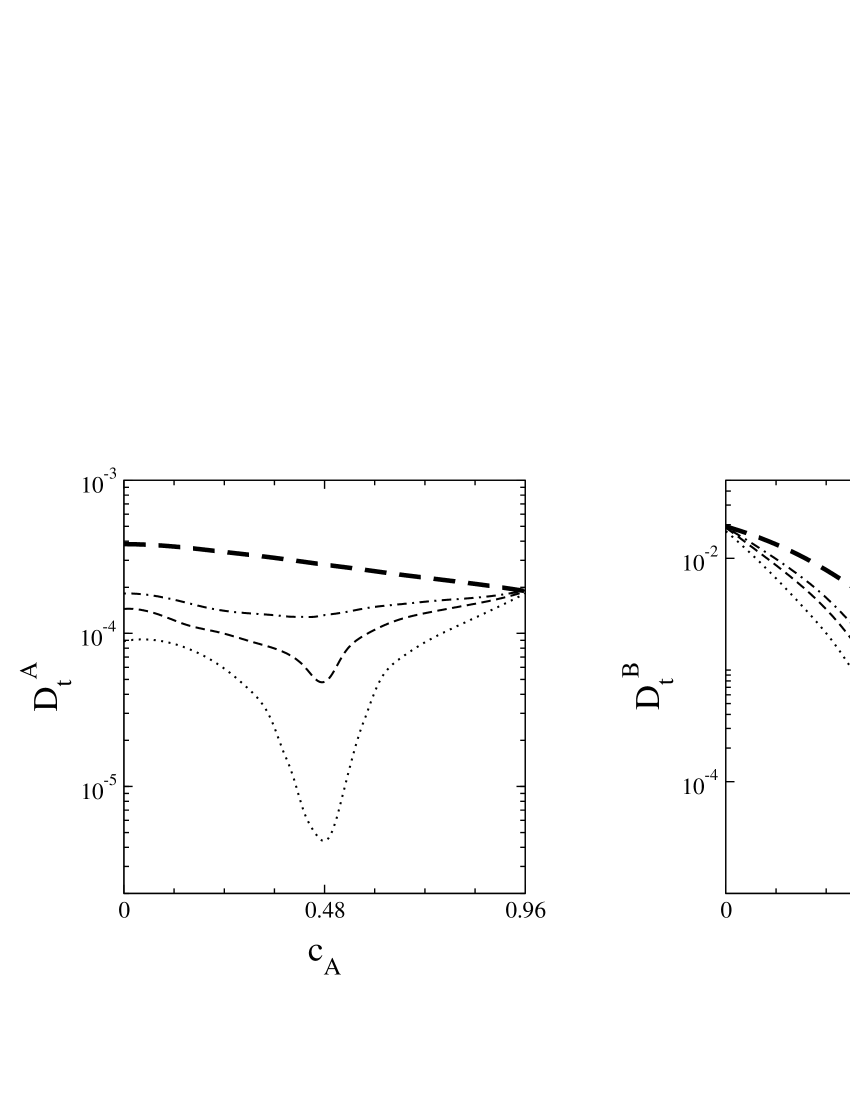
Figure 9: Tracer diffusion coefficients for $A$ particles (left) and $B$ particles (right), as a function of the concentration $c_{A}$. The jump rates are $\Gamma_{A}/\Gamma_{B}=0.01$ and several temperatures are considered: $T=0.6$ (dotted line), $T=0.912$ (dashed line) and $T=1.2$ (dot-dashed line). The thick line indicates in both cases the noninteracting, infinite temperature limit (random alloy model).

We start with a discussion of the tracer diffusion coefficients (Figs. 8, 9). The simplest case refers to equal jump rates $\Gamma_{A}=\Gamma_{B}=1$ of both types of particles $A$ and $B$ (Fig. 8). In the infinite temperature limit then there is no longer any physical difference between $A$ and $B$ particles, they simply differ only by their labels: then $D_{t}^{A}=D_{t}^{B}$, and become independent of concentration $c_{A}$ (thick horizontal straight line in Fig. 8). Note that for $c_{A}=0.96$ there are no $B$ particles since $c_{V}=0.04$ and then $D_{t}^{A}$ becomes independent of temperature, similarly as $D_{t}^{B}$ becomes independent of temperature for $c_{A}=0$. Of course, the curves for $D_{t}^{B}$ are simply the mirror images of those for $D_{t}^{A}$ around the symmetry line $c_{A,max}^{crit}=(1-c_{V})/2=0.48$ of the static phase diagram, Fig. 2b, since an interchange of $A$ and $B$ means that $c_{A}$ gets replaced by $1-c_{V}-c_{B}$.

It is seen that the onset of ordering depresses self-diffusion very strongly, while short range order (as it occurs for $T=1.2$) has a minor effect only. For $T=0.6$, however,the ordering near $c_{A}=0.48$ is rather perfect and there deep minima of $D_{t}^{A},D_{t}^{B}$ occur, the tracer diffusion coefficients decrease by about two orders of magnitude. Of course, since $D_{t}^{A},D_{t}^{B}$ are not symmetric around $c_{A,max}^{crit}=c_{B,max}^{crit}=(1-c_{V})/2=0.48$, due to the choice of a kinetic Monte Carlo algorithm which lacks the symmetry between the motion of an $A$ particle, mediated by a vacancy, in a $B$ environment and in an $A$ environment at finite temperatures, the minimum of $D_{t}^{A}$ does not occur precisely at $c_{A,max}^{crit}$, as is seen from Fig. 8 (left part). In our algorithm, an $A$ particle jumps to a vacant site with a jump rate $\Gamma_{A}\exp(-\Delta n|\epsilon_{AB}|/k_{B}T)$ when the difference between the number of $AB$ bonds involving an energy $\epsilon_{AB}$ each between the initial and final state is $\Delta n>0$, and with a jump rate $\Gamma_{A}$ else. It is easy to be convinced that this algorithm satisfies detailed balance with the canonic equilibrium distribution, as it should be 19 . In the limit $c_{A}\rightarrow 1-c_{V}$, we always have $\Delta n=0$, so there is no temperature dependence. In the limit $c_{A}\rightarrow 0$, however, every $A$ atom not having a vacancy as nearest neighbors will have four $B$ neighbors on the square lattice, while an $A$ atom with a vacancy neighbor has only three $B$ neighbors. As a result, the jump of an $A$ atom that has a $B$ neighbor, to a vacant site involves “breaking” an $AB$ bond, and hence this rate is suppressed by a factor $\exp(-|\epsilon_{AB}|/k_{B}T)$. This effect is responsible for the temperature dependence of $D_{t}^{A}$ for $c_{A}\rightarrow 0$.

Kehr et al. 17 presented arguments to relate the tracer diffusion coefficients to Onsager coefficients which take a simple form in the case of identical jump rates $\Gamma_{A},\Gamma_{B}$, namely

$$D_{t}^{A}=\Lambda_{AA}/c_{A}-\Lambda_{BA}/c_{B},\quad D_{t}^{B}=\Lambda_{BB}/c_{B}-\Lambda_{AB}/c_{A}$$ (41)

Using our estimates for the Onsager coefficients at $T=0.6$ (see below) in Eq. (41), one sees that the trend of the concentration dependence of $D_{t}^{A}$ is reproduced rather well. However, one should note that the derivation of Eq. (41) is rigorous only for the special case $\epsilon_{AB}/k_{B}T=0$, because only then the distinction between $A$ and $B$ particles forming the environment of a tagged $A$ particle can be neglected.

When $\Gamma_{A}\neq\Gamma_{B}$ the self-diffusion coefficients $D_{t}^{A}$ and $D_{t}^{B}$ lack any symmetric relation of their concentration dependence already in the random alloy limit 17 , and for $\epsilon_{AB}/k_{B}T<0$ we are not aware of any theoretical treatment to which our simulation results (Fig. 9) could be compared. Interestingly, for not too low temperatures (such as $T=0.912$, $T=1.2$) the concentration dependence of $D_{t}^{A}$ (the slower diffusing species, since $\Gamma_{A}/\Gamma_{B}=0.01$ has been chosen in Fig. 9) is rather weak throughout, while for $D_{t}^{B}$ we have a strong decrease when $c_{A}$ increases up to about $c_{A,max}^{crit}=0.48$. For $c_{A}>c_{A,max}^{crit}$ again a very weak concentration dependence results. For $T=0.6$ again pronounced minima near $c_{A,max}^{crit}$ are seen. Now, for $D_{t}^{B}$ we have a strong decrease when $c_{A}$ increases up to about $c_{A,max}^{crit}$, while for $c_{A}>c_{A,max}^{crit}$ again a very weak concentration dependence results.

Moreover, when for $c_{A}=c_{A,max}^{crit}$ the order of the $AB-$ checkerboard structure is perfect (apart from a four per cent of vacant sites in the system), a jump of an atom to a vacant site occurs with rates $\Gamma_{A}\exp(3\epsilon_{AB}/k_{B}T)$ or $\Gamma_{B}\exp(3\epsilon_{AB}/k_{B}T)$, respectively, while the backward jump occurs at rates $\Gamma_{A},\Gamma_{B}$. As a result, a high probability for backward jumps is expected, and this is borne out by a study of the correlation factor $f$ for self-diffusion (Fig. 10, right part). Following standard treatments 1 ; 2 ; 3 ; 4 ; 5 ; 6 ; 23 we decompose tracer diffusion coefficients $D_{t}$ as

$$D_{t}=VWf\;,$$ (42)

where $V$ is the vacancy availability factor already defined in Eq. (9), and $W$ is the average jump rate for the considered particle species. $W$ is easily estimated in the simulation from the ratio of the number of performed jumps to the number of all attempted jumps. The product $V_{A}W_{A}$ is plotted in Fig. 10 (left part) versus $c_{A}$ at various temperatures. For $\epsilon_{AB}/k_{B}T\rightarrow 0$ we simply expect a horizontal straight line, $V_{A}W_{A}=0.04$, since then $W_{A}=1$, $V_{A}=c_{V}$ ($\alpha_{1}=0$). There is no independent way to determine $f$, however. Therefore Eq. (42) is taken as a definition of $f$, to be derived from $D_{t}$, while the tracer diffusion constants are estimated from the mean square displacements of the tagged particles, as explained in Sec. III of this paper. For $c_{A}\rightarrow 0.96$, when no $B$ particles are present, the temperature dependence drops out and $f$ reduces to the value $f=0.487$ known from studies of a one-component non-interacting lattice gas on a square lattice with concentration $c_{A}=0.96$ 28 . Note that our data for $D_{t}$, $V$, $W$ and $f$ at the higher temperatures (where no order-disorder transition occurs) resemble analogous results of Murch 25 for a simple cubic alloy.

As a final comment about self-diffusion, we consider the temperature dependence of $D_{t}^{A}$ and $D_{t}^{B}$ for the critical concentration $c_{A}^{crit}=c_{B}^{crit}=0.48$ (Fig. 11). One sees that at high temperatures ($T\geq 2T_{c}$) the temperature dependence is very weak, and the tracer diffusion coefficients settle down at their infinite temperature asymptotes. Approaching the critical point one sees a more rapid decrease of both $D_{t}^{A}$ and $D_{t}^{B}$, with a maximum slope presumably right at $T_{c}$, while for $T$ below $T_{c}$ a crossover to the expected thermally activated behavior at low temperatures occurs. In fact, one expects that $D_{t}-D_{t}^{*}\propto(T-T_{c})^{1-\alpha}$ 24 , where $D_{t}^{*}$ is the value of the tracer diffusion coefficient at the critical point, and $\alpha$ is the specific heat exponent of the model. However, for the two-dimensional Ising model $\alpha=0$ 32 ; 33 ; 34 , i.e. the specific heat has a logarithmic singularity only. The insert of Fig. 11 shows a log-log plot of $D_{t}-D_{t}^{*}$ versus $(T-T_{c})/T_{c}$, and one sees that the data are compatible with a power law with slope of unity; presumably the accuracy of our simulations does not suffice to identify the presence of a logarithmic singularity in our data.

V.2 Onsager coefficients

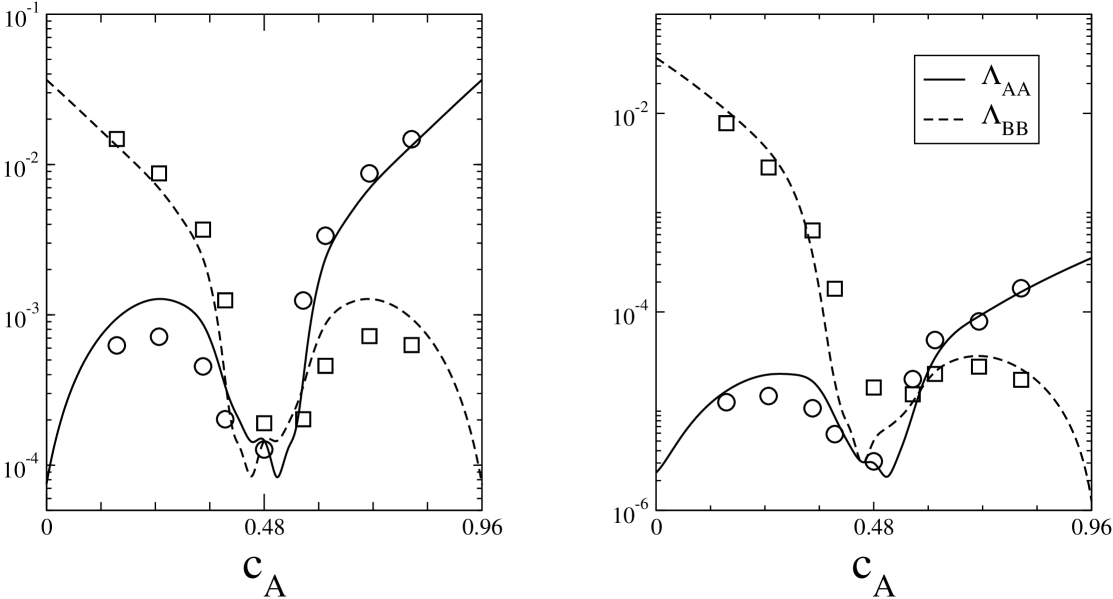
Figure 12: Plot of the Onsager coefficients $\Lambda_{ii}$ as a function of the concentration $c_{A}$, for a fixed temperature $T=0.6$. The jump rates are $\Gamma_{A}=\Gamma_{B}=1$ (left) and $\Gamma_{A}/\Gamma_{B}=0.01$ (right). The lines correspond to data obtained directly from the simulations, while the points correspond to the estimates obtained after using the aproximation of Eq. (43) for the random alloy model.

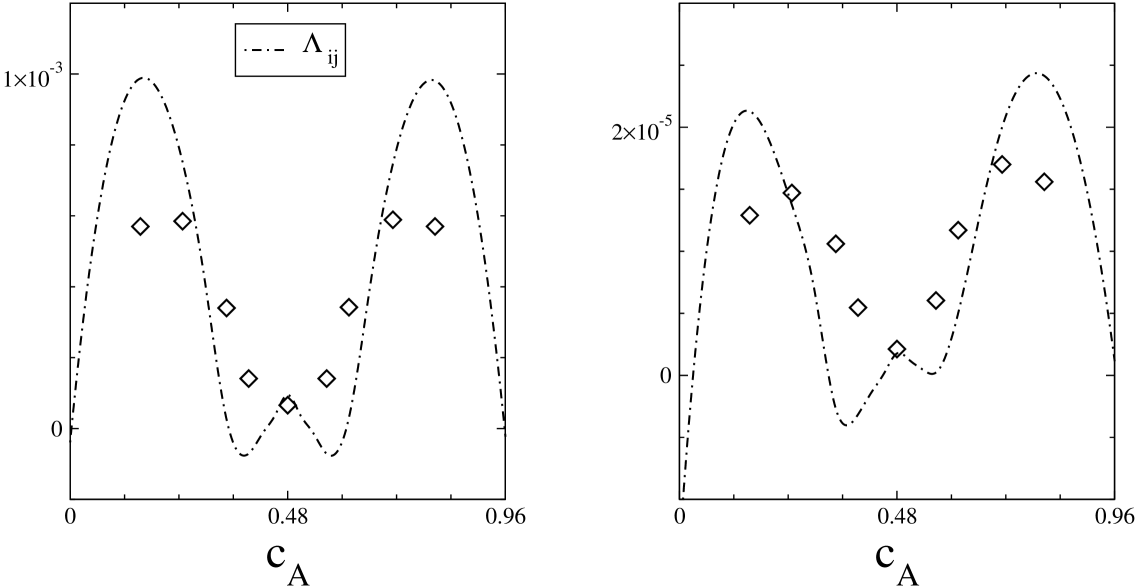
Figure 13: The same as figure 12 but here the crossed coefficient $\Lambda_{ij}$ is shown.

As a first issue of this subsection, we turn to the concentration dependence of the Onsager coefficients (Figs. 12, 13). For $\Gamma_{A}=\Gamma_{B}$ all Onsager coefficients are symmetric around $c_{A}=c_{B}=(1-c_{V})/2$, as it must be, while for $\Gamma_{A}\neq\Gamma_{B}$ they are not. We have also included an approximate relation suggested by Kehr et al. 17 between Onsager coefficients and tracer diffusion coefficients, namely

$$\Lambda_{\alpha\beta}=c_{\alpha}D_{t}^{\alpha}\;\left[\delta_{\alpha\beta}+\frac{1-f(c)}{f(c)}\,\frac{c_{\beta}D_{t}^{\beta}}{\sum\limits_{\gamma}c_{\gamma}D_{t}^{\gamma}}\right],$$ (43)

where $c=c_{A}+c_{B}$, $f(c)$ being the correlation factor for tagged-particle diffusion in a lattice gas with summary concentration $c$. It is seen that this relation accounts for the general trend of the diagonal Onsager coefficients rather well, although for the off-diagonal Onsager coefficient it seems to work only qualitatively (Fig. 13). In the regime of the ordered phase the diagonal Onsager coefficients (note the logarithmic ordinate scale) are distinctly smaller than for $c_{A}\rightarrow 0$ or $c_{B}\rightarrow 0$, respectively, when $\Gamma_{A}=\Gamma_{B}$.

An interesting aspect of the off-diagonal Onsager coefficient $\Lambda_{AB}=\Lambda_{BA}$ (Fig. 13) is that it is essentially zero for $c_{A}\rightarrow 0$ if $\Gamma_{A}=\Gamma_{B}$ while for $\Gamma_{A}/\Gamma_{B}=0.01$ it is essentially negative in this limit. A negative Onsager coefficient means that the currents of $A$ and $B$ particles are oriented in the opposite direction. A further change of sign of this off-diagonal coefficient is found near the phase boundary of the order-disorder transition; but near $c_{A}=c_{B}=(1-c_{V})/2$ the Onsager coefficient seems to be positive again, although its absolute value seems to be very small. We do not have any clear physical interpretation for this surprising behavior. Note also, that Eq. (43) can never yield a negative Onsager coefficient, since $0\leq f(c)\leq 1$ by definition, and hence all terms in Eq. 43 are non-negative.

Finally Fig. 14 shows the temperature dependence of the Onsager coefficients for the concentration $c_{A}=c_{B}=(1-c_{V})/2$ where the critical temperature $T_{c}$ of the order-disorder transition is maximal. Note that for $\Gamma_{A}/\Gamma_{B}=0.01$ the magnitude of the off-diagonal Onsager coefficient $\Lambda_{AB}$ is comparable to the smaller ($\Lambda_{AA}$) of the diagonal ones, both at very high and at very low temperatures. This finding confirms the conclusion of Kehr et al. 17 , that in general the off-diagonal Onsager coefficient must not be neglected. We also note that the general trend of the temperature dependence of the Onsager coefficients is very similar to the behavior of the self-diffusion coefficient, see Fig. 11. Both quantities reflect the strong decrease of mobility of the particles at low temperatures.

V.3 Interdiffusion

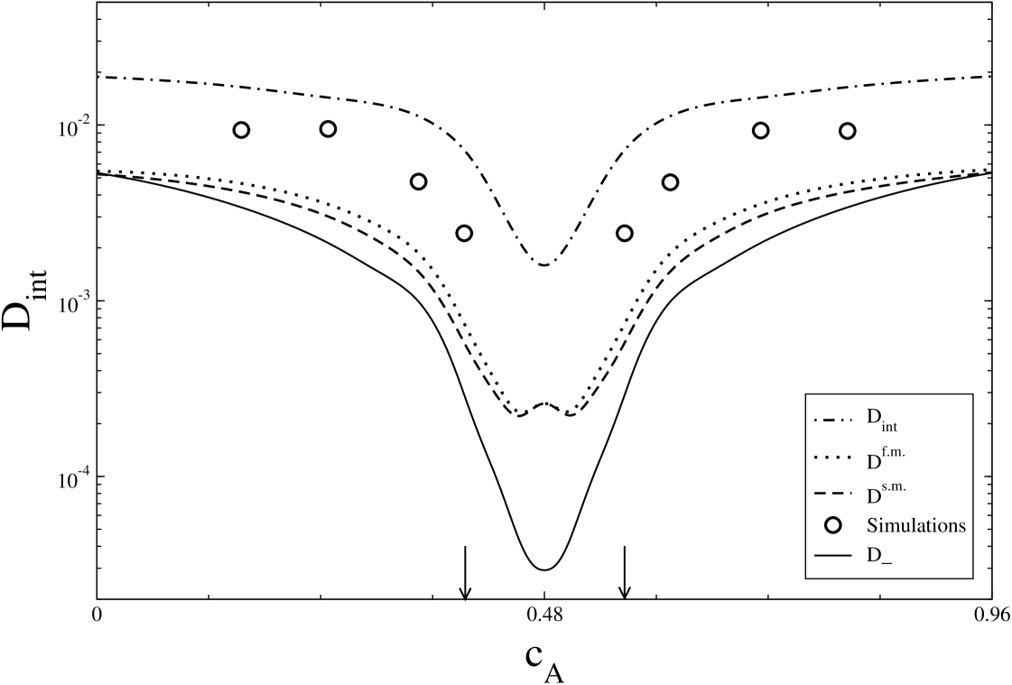
Figure 15: Plots of the interdiffusion coefficient as a function of the concentration $c_{A}$, for a temperature $T=0.6$. The jump rates are $\Gamma_{A}=\Gamma_{B}=1$. The arrows mark the corresponding critical values of $c_{A}$ for this temperature. Simulation results are compared to different theoretical approaches, for a discussion see the text.

Fig 15 presents a plot of the interdiffusion constant $D_{int}$ vs. concentration for the case of equal jump rates ($\Gamma_{A}=\Gamma_{B}=\Gamma=1$) at $T=0.6$ and compares the results to various analytical approximations: $D_{-}$ (Eq. (32)), the “slow mode” expression $D_{int}^{s.m.}$ (Eq. (38)), the “fast mode” expression $D_{int}^{f.m.}$ (Eq. (40)), and a very simple result justified by Kehr et al. 17 for the non-interacting random alloy model,

$$D_{int}^{n.i.}=(1-c)\,f(c)\,\Gamma\;.$$ (44)

While this last expression overestimates the numerical results, all other expressions underestimate them significantly. It is seen that in this case there is not much difference between the slow mode and fast mode theory, but both are off from the data. In this case using the full expression (Eq. (32)) presents no improvement, unlike the non-interacting case. Of course, at finite temperature in $d=2$ the mean field theory implicit in Eq. (32) is not expected to be accurate at all.

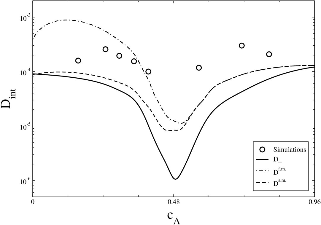
Figure 16: Plots of the interdiffusion coefficient as a function of the concentration $c_{A}$, for a temperature $T=0.6$. The jump rates are $\Gamma_{A}/\Gamma_{B}=0.01$.

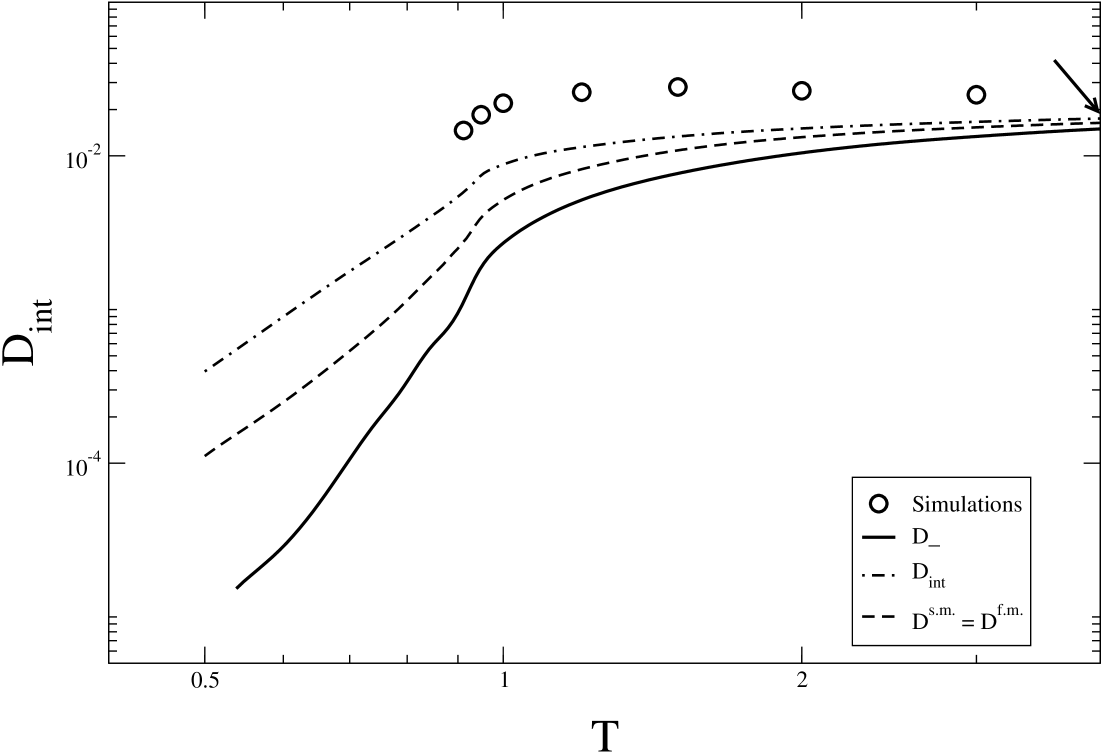
Figure 17: Logarithmic plot of the interdiffusion coefficient as a function of the temperature, for a concentration $c_{A}=c_{B}=0.48$. The jump rates are $\Gamma_{A}=\Gamma_{B}=1$. The arrow marks the infinite temperature result, where all the quantities showed in the plot coincide.

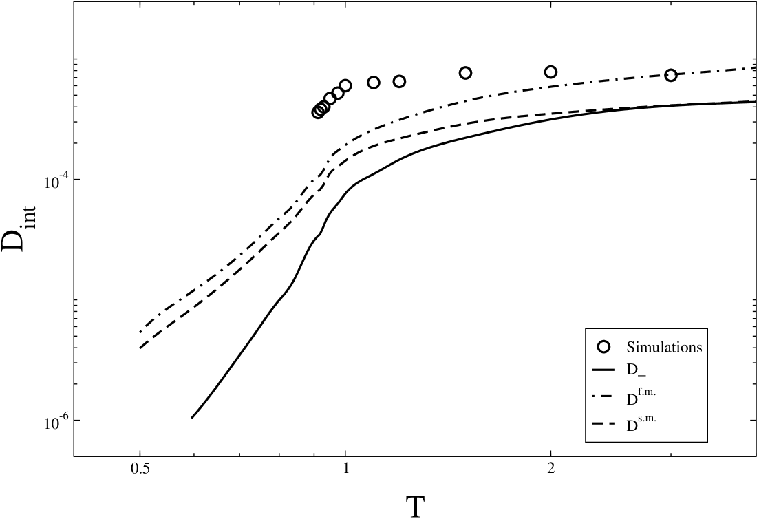
Figure 18: Logarithmic plot of the interdiffusion coefficient as a function of the temperature, for a concentration $c_{A}=c_{B}=0.48$. The jump rates are $\Gamma_{A}/\Gamma_{B}=0.01$.

It now is no surprise any longer that in the asymmetric case $\Gamma_{A}/\Gamma_{B}=0.01$ the various approximate expressions are not reliable either (Fig. 16). In particular, for concentrations near $c_{A}=c_{B}=(1-c_{V})/2=0.48$ a pronounced minimum is predicted, while the actual simulation results reveal a rather shallow minimum only. Again the conclusion is that there is no reliable simple relation between self-diffusion and interdiffusion coefficients, and the temperature dependence of $D_{int}$ at $c_{A}=c_{B}=0.48$ at higher temperatures (Figs. 17,18) confirms this conclusion. Again, for $\Gamma_{A}=\Gamma_{B}=\Gamma=1$ Eq. (44) is closest to the data, while Eq. (32) is worst. For $T\rightarrow\infty$, however, in this limit for $c_{A}=c_{B}=(1-c_{V})/2$ and $\Gamma_{A}=\Gamma_{B}=1$ all expressions coincide (at a value highlighted by an arrow in Fig. 17), and the numerical data have been found in good agreement with this prediction 17 . Thus it is clear that including interactions among the particles destroys the applicability of the simple theories.

VI CONCLUSIONS

In this paper, the study of mobility of particles, interdiffusion and tracer diffusion coefficients of a lattice model for a binary alloy, that was presented in Ref. 17 for the simple non-interacting limit only, has been extended to the case where an attractive nearest-neighbor interaction between unlike particles leads to an order-disorder transition on the considered square lattice. While most theoretical considerations of the previous work 17 can be simply extended to the present case, the mean-field character of the approximations that are involved clearly emerges as a severe limitation of the usefulness of all these approaches. On the other hand the Monte Carlo techniques described in Ref. 17 , suitable for the direct estimation of all Onsager coefficients and the interdiffusion constant $D_{int}$ as function of the ratio of jump rates $\Gamma_{A}/\Gamma_{B}$, temperature $T$ and concentration $c_{A}$, are rather straightforward to apply. Exploring this rather large parameter space numerically is however somewhat tedious, and an understanding of diffusion phenomena within the framework of lattice models for interacting particles by simple analytical expressions clearly would be desirable. However, the approximate expressions discussed in the present paper clearly do not give qualitatively accurate results.

Of course, the present study is a first step only: in order to make closer contact with possible experiments in surface layers of metallic alloys, it would be interesting to consider other lattice symmetries (triangular and centered rectangular lattice rather than square lattices), further neighbors interactions, etc..

A very important extension would also be the inclusion of asymmetric effects ($\epsilon_{AA}\neq\epsilon_{BB}$) and nonzero energy parameters involving vacancies ($\epsilon_{AV},\epsilon_{BV},\epsilon_{VV}$). Thus effects could be described that vacancies occupy preferentially sites at interfaces 21 or in one of the sublattices ecm . Such effects are expected to modify the diffusion behavior significantly.

We thus hope the present study will stimulate the development of more accurate theoretical descriptions of diffusion phenomena in alloys that undergo order-disorder transitions. Also corresponding experiments studying a wide range of temperature and composition, would be desirable. Then it might be worthwhile to combine the present kinetic Monte Carlo methodology with “ab initio” calculation of jump rates, ordering energies $\epsilon_{\alpha\beta}$, etc.

Acknowledgements: One of us (A.D.V.) is grateful to the German Academic Exchange Service (DAAD) and to the Deutsche Forschungsgemeinschaft (DFG), grant No SFB TR6/A5, for financial support.

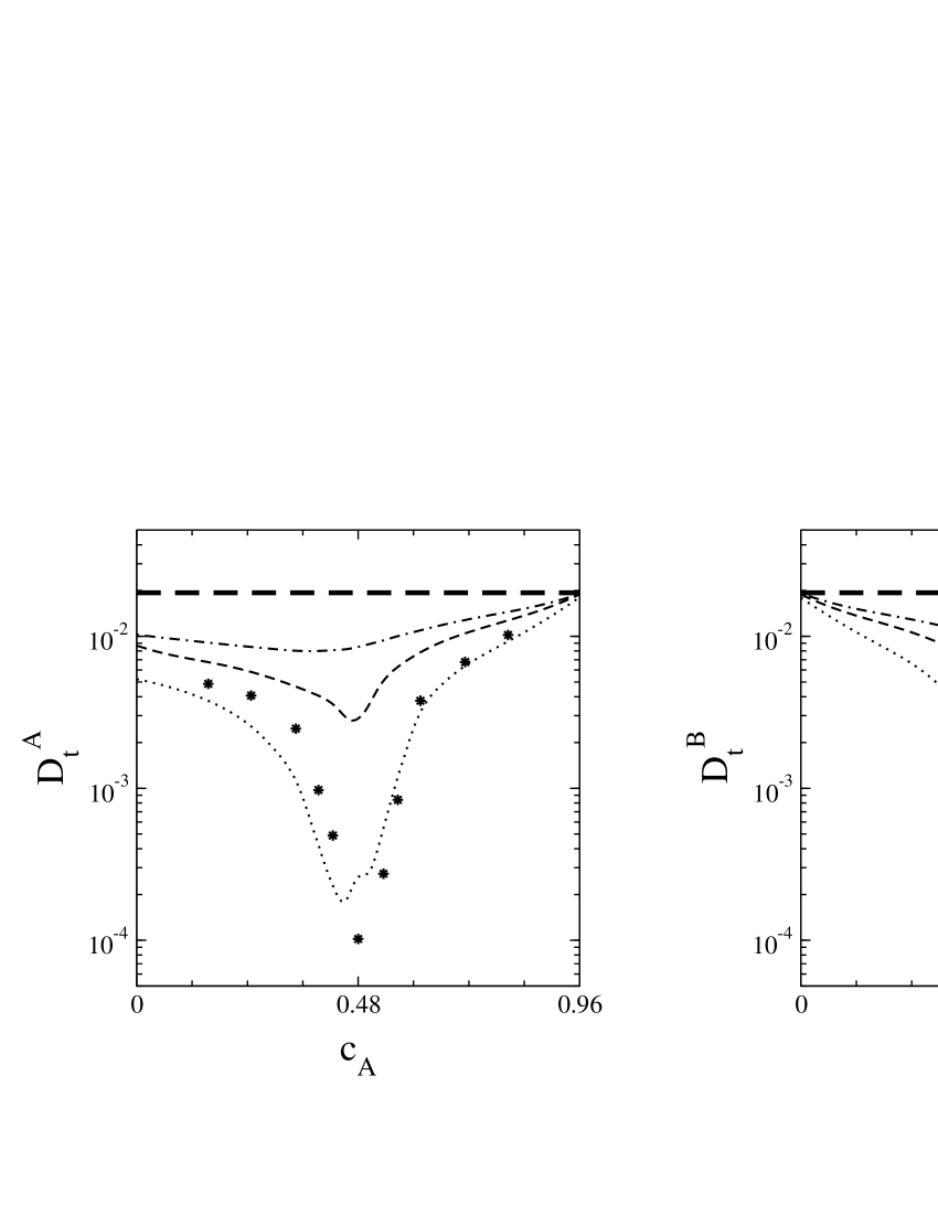
Figure 8: Tracer diffusion coefficients for $A$ particles (left) and $B$ particles (right), as a function of the concentration $c_{A}$. The jump rates are $\Gamma_{A}=\Gamma_{B}=1$ and several temperatures are considered: $T=0.6$ (dotted line), $T=0.912$ (dashed line) and $T=1.2$ (dot-dashed line). The thick line indicates in both cases the noninteracting, infinite temperature limit (random alloy model). Dots represent results obtained from Eq. (41).

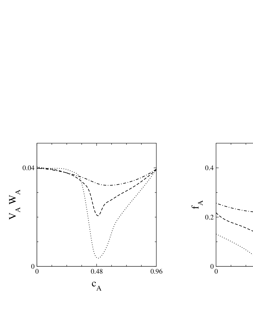
Figure 10: Effective jump rate (left) and correlation factor (right) for $A$ particles, as a function of the concentration $c_{A}$ and for different temperatures: $T=0.6$ (dot line), $T=0.91$ (dashed line) and $T=1.2$ (dot-dashed line). The jump rates are $\Gamma_{A}=\Gamma_{B}=1$.
The first quantity provides an idea of the rate at which jumps actually occur at a certain temperature and composition. It is defined as the product of the vacancy availability factor $V_{A}$ (related to the short-range order parameter $\alpha_{1}$) and the average jump rate $W_{A}$ (defined as the quotient of the number of performed jumps to the number of all attempted jumps). The $T\rightarrow\infty$ limit is given by $V=c_{v}\equiv 0.04$, because in this case $\alpha_{1}\equiv 0$.
Once we obtain $VW$ we can estimate the correlation factor $f$ applying the definition $D_{t}=VWf$ and using $D_{t}$ from Fig 8. See Refs. 23 ; 24 ; 25 ; 26 for details on the effect of correlations on tracer diffusion in lattice gas models.
The limit value $f=0.487$ for $c_{A}\rightarrow 0.96$ is known from Ref. 28 . This corresponds to a noninteracting, one-component lattice gas in a square lattice with concentration $c=0.96$.

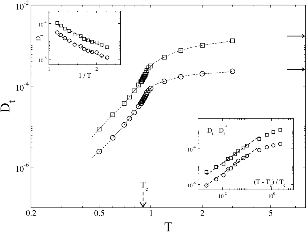
Figure 11: Dependence of the tracer diffusion coefficients on the temperature, for a stoichiometric composition $c_{A}=c_{B}=0.48$. The ratio of jump rates is $\Gamma_{A}/\Gamma_{B}=0.01$. Circles are $A$ particles and squares are $B$ particles.
The dashed arrow marks the critical temperature $T_{c}=0.905$ (in units of the Ising critical temperature), while the thick arrows indicate the asymptotic, infinite temperature values for both coefficients.
Inset (up): Arrhenius plot of $D_{t}$ for $T\ll T_{c}$. Inset (bottom): scaling plot of $|D_{t}-D_{t}^{*}|\sim|T-T_{c}|^{1-\alpha}$ with $\alpha=0$ (specific heat exponent of the Ising model). The dashed line has a slope of unity.

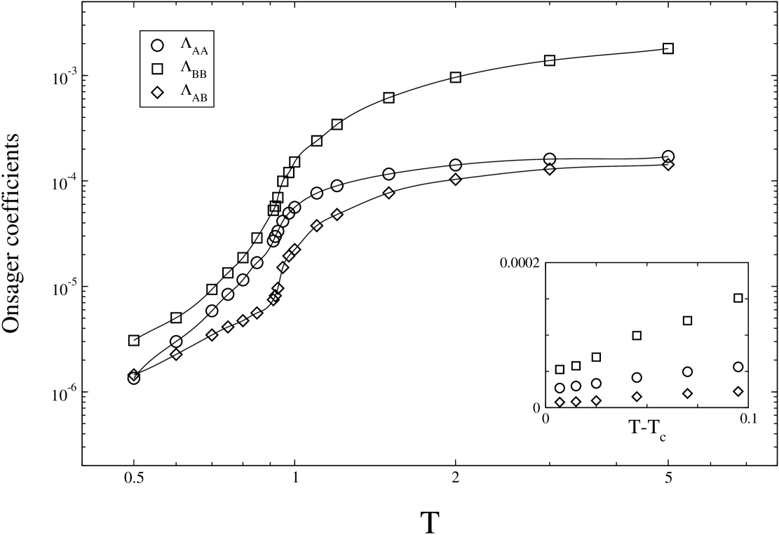
Figure 14: Plot of the Onsager coefficients $\Lambda_{ij}$ as a function of the temperature, for a stoichiometric concentration $c_{A}=c_{B}=0.48$ and jump rates $\Gamma_{A}/\Gamma_{B}=0.01$. The lines are drawn to guide the eyes.
Inset: plot of the same coefficients in the vicinity of the critical temperature, showing the linear approach to finite values right at $T_{c}$.

References

- (1) R. E. Howard and B. B. Lidiard, Rep. Progr. Phys. 27, 161 (1964)
- (2) J. R. Manning, Diffusion Kinetics for Atoms in Crystals (Van Nostrand, Princeton, 1968)
- (3) C. P. Flynn, Point Defects and Diffusion (Clarendon, Oxford 1972)
- (4) W. van Gool (ed.) Fast Ion Transport in Solids (North-Holland, Amsterdam, 1973)
- (5) G. E. Murch, Atomic Diffusion Theory in Highly Defective Solids (Trans Tech House, Adermannsdorf, 1980)
- (6) A. R. Allnatt and A. B. Lidiard, Rep. Prog. Phys. 50, 373 (1987)
- (7) R. J. Borg and G. J. Dienes, An Introduction to Solid-State Diffusion (Academic Press, NY, 1988)
- (8) G. E. Murch (Ed.) Diffusion in Solids: Unsolved Probems (Trans Tech Publ. Zürich, 1992)
- (9) J. Kärger, P. Heitjans, and R. Haberlandt (Eds.) Diffusion in Condensed Matter (Vieweg, Wiesbaden, 1998)
- (10) R. van Gastel, E. Somfai, S. B. van Albada, W. van Saarloos, and J. W. M. Frenken, Phys. Rev. Lett. 86, 1562 (2001)
- (11) M. L. Grant, B. S. Swartzentruber, N. C. Bartelt, and S. B. Hannon, Phys. Rev. Lett. 86, 4588 (2001)
- (12) M. L. Anderson, M. J. D’Amato, P. J. Feibelmann, and B. S. Swartzentruber, Phys. Rev. Lett. 90, 126102 (2003)
- (13) A. van der Ven and G. Ceder, Phys. Rev. Lett. 94, 045901 (2005)
- (14) D. DeFontaine, in Solid State Physics, Vol. 34, p. 73 (Academic Press, New York, 1979)
- (15) K. Binder, in Materials Science and Technology, Vol. 5 (P. Haasen, ed.) (Wiley, Weinheim, 1991) p. 143
- (16) G. Kostorz (ed.) Phase Transformations in Materials (Wiley-VCH, Berlin, 2001); P. E. A. Turchi and A. Gonis (eds.) Statics and Dynamics of Alloy Phase Transformations (Plenum Press, New York, 1996)
- (17) K. W. Kehr, K. Binder, and S. M. Reulein, Phys. Rev. B 39, 4891 (1989)
- (18) M. C. Tringides (Ed.) Surface Diffusion. Atomistic and Collective Processes (Plenum, New York, 1997)
- (19) D. P. Landau and K. Binder, A Guide to Monte Carlo Simulations in Statistical Physics, 2nd ed. (Cambridge, Univ. Press, Cambridge, 2005)
- (20) M. Porta, E. Vives and T. Castan, Phys. Rev. B 60, 3920 (1999) and references therein
- (21) J. Yuhara, M. Schmid, and P. Varga, Phys. Rev. B 67, 195407 (2003), and references therein
- (22) K. Yaldram and K. Binder, Acta Metall. 39, 707 (1991); J. Stat. Phys. 62, 161 (1991); Z. Physik B 82, 405 (1991)
- (23) G. E. Murch and R. J. Thorn, Philos. Mag. 35, 493 (1977); Philos. Mag. 35, 1441 (1977)
- (24) K. W. Kehr, R. Kutner, and K. Binder, Phys. Rev. B 23, 4931 (1981)
- (25) K. W. Kehr, R. Kutner, and K. Binder, Phys. Rev. B 26, 2967 (1982)
- (26) G. E. Murch, Philos. Mag. A 45, 941 (1982); Ibid. 46, 565 (1982)
- (27) K. W. Kehr, R. Kutner and K. Binder, Phys. Rev. B 28, 1846 (1983)
- (28) A. Sadiq and K. Binder, Surf. Sci. 128, 350 (1983)
- (29) For an early review, see K. W. Kehr and K. Binder, in Applications of the Monte Carlo Method in Statistical Physics (K. Binder, ed.) p. 181 (Springer, Berlin, 1984)
- (30) L. Zhang, W. A. Oates and G. E. Murch, Phil. Mag. A 58, 937 (1989)
- (31) A. Ala-Nissila, R. Ferrando, and S. C. Ying, Adv. Phys. 51, 949 (2002)
- (32) G. Bester, B. Meyer and M. Fähnle, Phys. Rev. B 57, R11019 (1998); B. Meyer and M. Fähnle, Phys. Rev. B 59, 6072 (1999)
- (33) K. Binder, in Statics and Dynamics of Alloy Phase Transformations (P. E. A. Turchi and A. Gonis, eds) p. 467 (Plenum Press, New York, 1996)
- (34) L. Onsager, Phys. Rev. 65, 117 (1944)
- (35) B. M. McCoy and T. T. Wu, The Two-dimensional Ising Model (Harvard Univ. Press, Cambridge, 1973)
- (36) R. J. Baxter, Exactly Solved Models in Statistical Mechanics (Academic Press, London, 1982)
- (37) K. Binder and D. P. Landau, Phys. Rev. B 21, 1941 (1980)
- (38) K. Binder, Z. Phys. B 43, 119 (1981)
- (39) G. Kamienarz and H. W. J. Blöte, J. Phys. A: Math. Gen. 26, 201 (1993)
- (40) G. E. Murch, Phil. Mag. A 46, 151 (1982)
- (41) P. C. Hohenberg and B. I. Halperin, Rev. Mod. Phys. 49, 435 (1977)
- (42) F. Brochard, J. Jouffray and P. Levinson, Macromolecules 16, 1638 (1983)
- (43) K. Binder, J. Chem. Phys. 79, 6387 (1983); Colloid Polym. Sci. 265, 273 (1987)
- (44) K. Binder and H. Sillescu, in Encyclopaedia of Polymer Science and Engineering, 2nd ed. Suppl. Volume, edited by J. L. Kroschwitz (Wiley, New York, 1989)
- (45) W. Hess, G. Nägele, and A. Z. Akcasu, J. Poly. Sci. B: Pol. Phys. 28, 2233 (1990)
- (46) E. J. Kramer, P. Green, and C. J. Palmstrom, Polymer 25, 473 (1984)
- (47) H. Sillescu, Macromol. Chem. Rapid Comun. 5, 519 (1984); ibid 8, 393 (1983)
- (48) B. C. H. Steele, in Ref. 4, p. 103
- (49) J. W. Cahn and F. C. Larche, Scripta Met. 17, 927 (1983)