Orientational ordering in hard rectangles: the role of three-body correlations

Abstract

We investigate the effect of three-body correlations on the phase behavior of hard rectangle two-dimensional fluids. The third virial coefficient, $B_{3}$, is incorporated via an equation of state that recovers scaled particle theory for parallel hard rectangles. This coefficient, a functional of the orientational distribution function, is calculated by Monte Carlo integration, using an accurate parameterized distribution function, for various particle aspect ratios in the range $1-25$. A bifurcation analysis of the free energy calculated from the obtained equation of state is applied to find the isotropic (I)-uniaxial nematic (N_u) and isotropic-tetratic nematic (N_t) spinodals and to study the order of these phase transitions. We find that the relative stability of the N_t phase with respect to the isotropic phase is enhanced by the introduction of $B_{3}$. Finally, we have calculated the complete phase diagram using a variational procedure and compared the results with those obtained from scaled particle theory and with Monte Carlo simulations carried out for hard rectangles with various aspect ratios. The predictions of our proposed equation of state as regards the transition densities between the isotropic and orientationally ordered phases for small aspect ratios are in fair agreement with simulations. Also, the critical aspect ratio below which the N_t phase becomes stable is predicted to increase due to three-body correlations, although the corresponding value is underestimated with respect to simulation.

I Introduction

The (two-dimensional) hard-rectangle (HR) model has recently received some attention due to the possibility that a dense film of these particles exhibits spontaneous tetratic orderSchaklen ; Martinez-Raton ; Frenkel1 ; Donev . Additional interest originates from the fact that some types of organic molecular semiconductors are made of rectangularly shaped molecules; a notable example is the PTCDA molecule, films of which have recently been studied quite intensely PTCDA . Even though the interactions between these molecules involve high-order polar forces (e.g. quadrupolar forces) it is of interest to investigate theoretically the intrinsic order associated to purely excluded-volume effects with a view to predicting structural and thermodynamic properties of the film by incorporating other interactions via traditional perturbation theories. The system we investigate in the present work mimics an incommensurate film of these molecules with only excluded-volume interactions involved and in the regime where molecules are free to move in the film (i.e. fluid regime). Phases with two-dimensional crystalline order will be left for future work.

Recently monolayers of various macroscopically-sized particles have been studied using mechanical vibrations on the monolayer to induce motion Narayan . Even though this is an athermal, non-equilibrium system reaching steady-state configurations, these configurations are mainly driven by packing effects and should give the trend as to what types of order could be expected. In particular, tetratic order was observed in particles with sufficiently sharp corners, resembling rectangles, in contrast with particles such as discorectangles (projections of spherocylinders on the plane) which only exhibit nematic ordering, or basmati-rice grains, which in addition may have a smectic phase.

Apart from the possible interest in modelling the behaviour of monolayers made of molecules with technological interest, our investigations have the additional, more fundamental aim of elucidating the effect that three-body correlations have on the orientational properties of two-dimensional fluids. Onsager showed that for three-dimensional hard rod fluids in the limit of infinite aspect ratio (hard-needle limit), $\kappa\to\infty$ (with $\kappa\equiv L/\sigma$, $L$ and $\sigma$ being the length and width of the constituent particles), the ratio between the third virial coefficient and the second virial coefficient squared asymptotically vanishes, for the isotropic fluid, as $B_{3}/B_{2}^{2}\sim(\sigma/L)\log(L/\sigma)$ Onsager . Taking this result into account, he used a second-order virial expansion for the free energy as a functional of the orientational distribution function and obtained predictions for the isotropic (I)-nematic (N) phase-transition densities, exact in the above limit. By contrast, in two dimensions the above ratio between virial coefficients has the approximate limiting value of $0.514$ Tarjus , implying that three-body correlations might play a very important role in the isotropic fluid even in the hard-needle limit; this is in sharp contrast with the three-dimensional case. An investigation of the effect of these high-order correlations on orientational ordering seems therefore appropriate.

Since Onsager theory does not account for higher-than-two body correlations, an alternative theoretical approach is required. Scaled particle theory (SPT), first developed for a mixture of hard spheres Reiss and later extended to anisotropic particles Cotter ; Lasher ; Barboy , includes as a main ingredient the exact analytic expression for the second virial coefficient Isihara ; Kihara , but again the third is approximated assuming $B_{3}/B^{2}_{2}\to 0$ in the hard-needle limit, an assumption that is incorrect. Also, it has been shown that, for a variety of particle shapes in two dimensions, the fourth and fifth virial coefficients tend to negative values in the same limit Tarjus ; Rigby . Thus it may very well occur that in these cases the virial series exhibits poor convergence, and a natural question arises: how does the phase behavior of anisotropic hard convex two-dimensional fluids change when three- and higher-body correlations, neither of which are included in the standard Onsager and SPT approaches, are taken into account? One of the aims of the present article is to shed some light on this question. For this purpose we develop an equation of state (EOS) for HR which exactly includes two- and three-body correlations in the nematic fluid and recovers SPT in the case of perfectly aligned particles.

Recent investigations of the HR system have used the SPT approach Schaklen ; Martinez-Raton and Monte Carlo (MC) simulations Frenkel1 ; Donev to study its phase behavior. Aside from the usual isotropic-uniaxial nematic (N_u) transition, these works have shown that this peculiar system exhibits a continuous transition between the isotropic phase and a tetratic nematic (N_t) phase. The latter is an orientationally ordered phase but with $D_{4h}$ symmetry, i.e., the system is invariant under rotation of $\pi/2$. The SPT predicts that this phase is stable up to an aspect ratio $\kappa\approx 2.21$ and that the packing fraction values of the I-N_t transition are around 0.85. This is in disagreement Martinez-Raton with the I-N_t transition densities obtained from simulation for $\kappa=1$ and $2$ Frenkel1 ; Donev , which predicts values around 0.7. Considering the importance that high-body correlations may have on the phase behavior of two-dimensional hard-convex bodies, it is the second purpose of this article to apply our model (which includes three-body correlations) to calculate the phase diagram of HR and compare the results with those of SPT and MC simulations. The main features of the phase diagram are calculated using bifurcation theory for the I-N transition and also minimizing the nematic free energy functional resulting from our proposed EOS.

The article is organized as follows. In Section II we describe the theoretical model for a general two-dimensional hard-convex fluid as applied to the isotropic and nematic fluids. Section III is devoted to the results obtained from the analysis of the theory, and comparison is made with simulation results; also, the complete liquid-crystal phase diagram is presented. Finally, some conclusions are drawn in Section IV. The Appendix contains a detailed account of the bifurcation analysis and the minimization method used to analyse the phase behaviour of the model, together with some details on the computer simulations.

II Theory

In the present section we introduce the theoretical formalism necessary for the study of the phase behavior of the HR fluid. This includes the derivation of the EOS for the isotropic and nematic fluids, along with the corresponding free energy density. The phase behaviour of the model, to be presented in the next section, is analysed by means of two complementary techniques: a bifurcation analysis of the free energy density, and a full minimization using an accurate functional form for the orientational distribution function. Details on these techniques are given in the Appendix.

II.1 EOS for the isotropic fluid

In this section an equation of state for the isotropic phase, to be extended later to the nematic phase, is proposed, on a somewhat ad-hoc, but at the same well-founded, basis. The virial coefficients are intimately related to geometric properties of the planar objects making up the fluid. The second virial coefficient of planar hard particle has the analytic form Kihara

$$B_{2}=v+\frac{{\cal L}^{2}}{4\pi},$$ (1)

where $v$ and ${\cal L}$ are the area and perimeter of the particle. Some approximate analytic expressions for third virial coefficients of isotropic fluids made of three-dimensional bodies, as a function of their volume, surface area and mean curvature, have been proposed Boublik . When compared with results from numerical calculations Boublik , some of these expressions are seen to constitute accurate approximations. In two dimensions volume has to be substituted by area, area by perimeter and mean curvature by a function proportional to the perimeter (the latter is true for the most representative two-dimensional convex bodies, i.e. rectangles, discorectangles, and ellipses). Following some of the most successful approximations Boublik but translated to the two-dimensional case, we write the following analytic expression for the third virial coefficient

$$B_{3}=v^{2}+\frac{\alpha}{4\pi}v{\cal L}^{2}+\frac{\beta}{(4\pi)^{2}}{\cal L}^{4}$$ (2)

where the numerical coefficients $\alpha$ and $\beta$ are chosen in such a way as to guarantee i) the correct asymptotic hard-needle limit, and ii) a good comparison with well-known EOS for some isotropic fluids, such as hard disks. For the latter we have ${\cal L}^{2}=4\pi v$ so that the three terms in the right-hand side of Eqn. (2) can be unified into the single term $(1+\alpha+\beta)v^{2}$. The SPT for hard disks is recovered by choosing $\alpha+\beta=2$, whereas the SPT form for $B_{3}$ for a general anisotropic particle is obtained from (2) with $\alpha=2$ and $\beta=0$. Note, from Eqns. (1) and (2), that

$$B_{2}\sim\frac{{\cal L}^{2}}{4\pi},\quad B_{3}\sim\frac{\beta}{(4\pi)^{2}}{\cal L}^{4},$$ (3)

in the infinite aspect-ratio limit, as the particle area is proportional to the product of the two characteristic lengths of the particle (the width $\sigma$ and the length $L$, the latter being the larger one), while the perimeter is proportional to their sum. Therefore we obtain the asymptotic limit $B_{3}/B_{2}^{2}\to\beta$ when $L/\sigma\to\infty$ and a sensible choice is $\beta=0.514$, the exact asymptotic value of this ratio Tarjus .

The EOS is obtained by imposing two requirements: (i) the divergence of pressure at high packing fractions is of the form $\sim(1-\eta)^{-2}$ as stated by SPT, and (ii) the second and third virial coefficients are obtained from the exact virial expansion

$$\beta P = \rho+\rho^{2}B_{2}+\rho^{3}B_{3},$$ (4)

(where $\rho$ is the density of particles). In other words, we require that the third-order virial expansion of the interaction part of the EOS,

$$\beta P_{\rm{exc}}v=\beta Pv-\eta=\frac{a_{2}\eta^{2}+a_{3}\eta^{3}}{(1-\eta)^{2}},$$ (5)

($\eta=\rho v$ being the packing fraction) coincides with the exact one (4). This allows us to obtain $a_{k}$ ($k=1,2$) as $a_{2}=1+b_{2}$, and $a_{3}=b_{3}-2a_{2}-1$, where the new coefficients

$$b_{k}=\frac{B_{k}}{v^{k-1}}-1,\quad k=2,3,$$ (6)

have been defined in terms of the virial coefficients $B_{k}$. The resulting EOS has the form

$$\beta Pv=\frac{\eta}{1-\eta}+\frac{\eta^{2}}{(1-\eta)^{2}}+\frac{\eta^{3}}{(1-\eta)^{2}}\left(b_{3}-2b_{2}\right)$$ (7)

From this EOS the free energy density can be obtained: we first write

$$\rho^{2}\frac{\partial\varphi}{\partial\rho}=\beta P(\rho),$$ (8)

where $\varphi=\varphi_{\rm{id}}+\varphi_{\rm{ex}}$ is the free energy per particle and $\varphi_{\rm{id}}$ and $\varphi_{\rm{ex}}$ the corresponding ideal and excess contributions. Now using $\beta P$ from (7), Eqn. (8) can be integrated to give

$$\varphi_{\rm{exc}} = -\ln(1-\eta)+\frac{\eta}{1-\eta}b_{2}+(b_{3}-2b_{2})\theta(\eta),$$ (9)

$$\theta(\eta) = \frac{\eta}{1-\eta}+\ln(1-\eta)$$ (10)

The first two terms of (7) and (9) are SPT-like terms. Eq. (7), with the exact second and third virial coefficients for the particular case of parallel hard rectagles, recovers the SPT result [this is easily obtained if we substitute the exact values $B_{2}=2v$ ($b_{2}=1$) and $B_{3}=3v^{2}$ ($b_{3}=2$) in Eq. (7)].

Inserting $B_{2}$ and the approximation for $B_{3}$ from (1) and (2), respectively, in Eqns. (7) and (9), we obtain our proposed EOS and the excess part of the free energy per particle for the isotropic fluid as

$$\beta Pv = \frac{\eta}{1-\eta}+\frac{\eta^{2}}{(1-\eta)^{2}}\gamma\left[1+(\alpha-2+\beta\gamma)\eta\right],$$ (11)

$$\varphi_{\rm{ex}} = -\ln(1-\eta)+\frac{\gamma\eta}{1-\eta}+\gamma(\alpha-2+\beta\gamma)\theta(\eta),$$

where the anisometric parameter $\gamma={\cal L}^{2}/(4\pi v)$ was defined. Note that for $\alpha=2$, $\beta=0$, this equation recovers the SPT expression for hard convex bodies. From (11) the following expression for the reduced virial coefficients is obtained:

$$B_{n}^{*}\equiv\frac{B_{n}}{B_{2}^{n-1}}=\frac{1+\left[1+(\alpha-1)(n-2)\right]\gamma+\beta(n-2)\gamma^{2}}{(1+\gamma)^{n-1}}$$

(13)

II.2 EOS for the nematic fluid

The EOS for the nematic fluid is now obtained from Eqn. (7) by substituting the virial coefficients of the isotropic fluid $B_{n}$ ($n=2,3$) by their functional versions $B_{n}[h]$ for the nematic fluid; here $h(\phi)$ is the orientational distribution function. The latter coefficients are obtained from the definitions of $B_{2}$ and $B_{3}$, in terms of integrals over the Mayer function:

$$B_{k}[h]=\frac{1}{k}\left[\prod_{l=1}^{k}\int d\phi_{l}h(\phi_{l})\right]{\cal K}(\phi_{1},\dots,\phi_{k}),$$ (14)

$${\cal K}(\phi_{1},\phi_{2})=-\int d{\bf r}f({\bf r},\phi_{12}),$$ (15)

$${\cal K}(\phi_{1},\phi_{2},\phi_{3})=-\int d{\bf r}\int d{\bf r}^{\prime}f({\bf r},\phi_{12})f({\bf r}^{\prime},\phi_{23})$$

$$\times f({\bf r}-{\bf r}^{\prime},\phi_{13}),$$ (16)

where $\phi_{\alpha\beta}=\phi_{\alpha}-\phi_{\beta}$ is the relative angle between axes of particles $\alpha$ and $\beta$, and $f({\bf r},\phi_{\alpha\beta})$ the Mayer function. The corresponding free-energy functional $\varphi[h]=\varphi_{\rm{id}}[h]+\varphi_{\rm{ex}}[h]$ is obtained from Eqns. (9):

$$\varphi_{\rm{exc}}[h]=-\ln(1-\eta)+\frac{\eta}{1-\eta}b_{2}[h]+\left(b_{3}[h]-2b_{2}[h]\right)\theta(\eta)$$

(17)

with the ideal part exactly calculated from

$$\varphi_{\rm{id}}[h]=\ln\eta-1+\int_{0}^{2\pi}d\phi h(\phi)\ln\left[2\pi h(\phi)\right].$$ (18)

The remaining virial coefficients are approximated from Eq. (7) by

$$B_{n}[h]=v^{n-3}\left\{(n-2)B_{3}[h]-(n-3)B_{2}[h]v\right\}.$$ (19)

The integral over spatial variables in the definition of $B_{2}[h]$ is known analytically for most convex bodies. In particular, for HR we have

$${\cal K}(\phi_{1},\phi_{2})=\left(L^{2}+\sigma^{2}\right)|\sin\phi_{12}|+2L\sigma\left(1+|\cos\phi_{12}|\right),$$

which is the excluded area between particles with relative orientation $\phi_{12}$. However, the required double angular average over $h(\phi)$ has to be estimated numerically (we used Gaussian quadrature). Also, in the case of $B_{3}[h]$, all integrals have to be calculated numerically (using MC integration). For this purpose we found it convenient to use a parameterized orientational distribution function

$$h(\phi)=C\exp{\left(\sum_{\tau=1}^{n}\lambda_{\tau}\cos(2\tau\phi),\right)}$$ (21)

in terms of the $n$ parameters $\lambda_{\tau}$ ($\tau=1,\dots,n$). $C$ is a normalization constant. In practice two variational parameters ($n=2$) were used. Details on how this calculation was realized in practice are relegated to the Appendix.

III Results

In this section we present the main results obtained from the inclusion of three-body correlations into the EOS for the isotropic and the nematic fluids, as proposed in Section II. The results from bifurcation analysis and from numerical minimization of the free-energy functional are presented in Section III B. In the latter case we compare the results from the present theory with those obtained from SPT and from simulations. But before presenting the results, we show in Fig. 1 a series of particle snapshots extracted from our simulation runs. Details on the simulations are given later on. The three configurations are representative of an isotropic phase [Fig. 1(a)], a tetratic phase [Fig. 1(b)], and a crystalline phase [Fig. 1(c)].

Figure 1: Typical particle configurations as obtained from MC simulations. (a) isotropic phase; (b) tetratic phase; and (c) crystalline phase with particles arranged in one of the possible configurations. See text for details on the simulations.

III.1 Isotropic fluid

Let us first compare the different approximations for $B_{3}$ and assess their quality according to the degree of agreement with MC-integration results for isotropic fluids made of different hard-convex bodies. Our own MC calculations have been carried out for hard rectangles, while those of Ref. Rigby were focussed on hard discorectangles and hard ellipses. All the results are plotted in Fig. 2 along with two different analytic approximations for the reduced virial coefficient $B_{3}^{*}$. One of them (solid line) is calculated from Eqn. (13) with $\beta=0.514$ [which gives the correct value of $B_{3}$ in the Onsager limit Rigby –see Eqn. (3)], and setting $\alpha=1.611$, which gives the correct third virial coefficient for hard disks ($B_{3}^{*}\approx 3.125$). The other (dotted) line is also calculated from Eqn. (13), but choosing $\alpha=2$ and $\beta=1/8$, which reduces to the proposal made by Boublik in Ref. Boublik1 . As will be shown below, this proposal approximates the EOS for the isotropic phase of hard convex bodies reasonably well. Also plotted in Fig. 2 with dashed lines are the best fits calculated from

$$B_{3}=\delta_{\rm{HB}}v^{2}+\frac{\alpha_{\rm{HB}}}{4\pi}v{\cal L}^{2}+\frac{\beta_{\rm{HB}}}{(4\pi)^{2}}{\cal L}^{4}$$ (22)

with values for the coefficients $\delta_{\rm{HB}}$, $\alpha_{\rm{HB}}$, and $\beta_{\rm{HB}}$ depending on the particle geometry ($\rm{HB}\equiv HR,HDR,HE$), i.e. hard rectangles, hard discorectangles, and hard ellipses. Note that Eqn. (22) is the same as Eqn. (2), but with a new numerical coefficient $\delta_{\rm{HB}}$ as a prefactor of $v^{2}$. From Fig. 2 we can see that the present approximation ($\alpha=1.611,\beta=0.514$) describes the behavior of $B_{3}$ as a function of the anisometric parameter $\gamma$ much better than Boublik’s proposal which, in the Onsager limit, gives the (wrong) value $B_{3}^{*}=1/8$. Also, if one is to describe the correct behavior of $B_{3}^{*}$ for different particle geometries in the whole range of $\gamma$, it is necessary to take $\delta_{\rm{HB}}\neq 1$.

Numerical values for the coefficients $B_{4}^{*}$ and $B_{5}^{*}$ have been calculated in Ref. Rigby , for three different particle geometries, using MC integration. The results for $B_{4}^{*}$ are shown in Fig. 3. Also plotted are our analytic proposal (solid line) and that of Boublik (dotted line). For HR with small anisometry values our approximation is better than that of Boublik, while the opposite occurs for high anisometries. For hard ellipses, Boublik’s approach describes reasonably well the behavior of $B_{4}^{*}$ in the whole range of $\gamma$ (except for very long particles which have negative values of $B_{4}^{*}$).

Figure 2: Reduced virial coefficient $B_{3}^{*}$ as a function of the anisometric parameter $\gamma$. Simulation results are shown for hard rectangles (squares), discorectangles (asterisk), and ellipses (triangles). The solid and dotted lines are the results from Eq. (13) with $(\alpha,\beta)=(1.611,0.514)$, and $(\alpha,\beta)=(2,1/8)$ respectively. Also are shown with dashed lines the best fits from Eq. (22).

Figure 3: Reduced virial coefficient $B_{4}^{*}$ as a function of the anisometric parameter $\gamma$. All the lines and symbols label the same as in Fig. 2.

The EOS obtained from the above approximations can be checked against MC simulations of systems of HR particles. In order to realize this comparison we have carried out constant-pressure MC simulations on systems of HR with different aspect ratios in the range of pressures where the isotropic fluid is the stable phase. The results for $\kappa=3$ and 9 are shown in Figs. 4 (a) and (b), respectively. Simulations were done on systems of $\sim 10^{3}$ particles, equilibrated along typically $\sim 10^{6}$ MC steps, and averaging over $\sim 4\times 10^{6}$ MC steps. The system was prepared in each case in a crystalline low-density configuration with perfectly aligned particles at low pressure. This configuration rapidly turned into a disordered configuration, which was then equilibrated. After averaging, the system was subject to a higher pressure and then equilibrated, and the process was repeated increasing the pressure. In this way the EOS in the entire region of isotropic stability was obtained. For comparison we also show in Figs. 4 (a) and (b) the EOS corresponding to the SPT (dashed line), Boublik proposal (dotted line), our proposal (solid line) and the EOS [Eqn. (7)] with the virial coefficient $B_{3}$ calculated from MC integration. As can be seen the SPT and Boublik’s proposal approximate better the simulation results. However, given that both theories make wrong predictions of the behavior of the third and fourth virial coefficients of HR as a function of the anisometric parameter, these results are to be taken with caution in the sense that they could be a mere coincidence. We can also see from the figures that our proposal overestimates the pressure. This kind of behavior is typical of fluids composed of hard-core particles which exhibit poorly convergent virial series; this seems to be the case for HR particles since their fourth and fifth virial coefficients become negative for high anisometries.

Figure 4: Results from MC simulations (filled circles) on a system of 10800 HRs with $\kappa=3$ (a), and $\kappa=9$ (b). Dot-dashed line: Eq. (7) with $B_{3}$ calculated from MC integration, dashed line: SPT, dotted line: Boublik proposal, and solid line: our proposal [The $B3$ from Eq. (2) with $\{\alpha=1.611,\beta=0.514\}$].

III.2 Bifurcation to nematic fluid

We implemented numerically the bifurcation-theory analysis, described in detail in the Appendix, to calculate the spinodal instabilities from the isotropic phase to the N_u and N_t phases, and elucidated the order of these transitions within the same formalism. These results were checked against a full minimisation of the free-energy functional employing the methodology outlined in Section IIB, which in addition enabled the N${}_{t}-$N_u spinodals, which cannot be easily calculated using bifurcation theory, to be obtained. Also, in order to have essentially exact results for the phase behaviour of this system, we performed constant-pressure MC simulations on systems of $\sim 10^{3}-10^{4}$ HR particles and obtained the equations of state and orientational order (details on these simulations are included in Section D of the Appendix). All of these results are described in the following.

The I-N_u and I-N_t spinodal lines $\eta^{*}(\kappa)$ (the packing fraction at bifurcation as a function of the aspect ratio $\kappa$) were calculated by solving Eqn. (39) for $y=\eta/(1-\eta)$ (or $\eta$) for a discrete set of values of $\kappa$ (see Appendix). All the coefficients $b_{3}^{(k1,k2,k3)}$ that enter this equation were calculated via MC integration; typically $\sim 10^{8}$ MC steps were used to evaluate these coefficients. To elucidate the order of transitions, we solved Eqn. (46) to find (i) the value $\kappa_{1}$ at which the free energy difference between N_u or N_t and isotropic phases changes from negative to positive, which in turn reflects the change of sign of the coefficient $B^{*}$ (see Appendix), and (ii) the value $\kappa_{2}$ for which the inverse of the isothermal compressibility of the $N_{u}$ or $N_{t}$ phases [$\left(\kappa^{-1}_{\rm{N}}v\right)^{*}$] at the bifurcation point becomes zero. Again, all the coefficients $b_{3}$ (the rescaled third virial coefficient) and $b_{3}^{(k1,k2,k3)}$, necessary to solve Eqn. (46), were evaluated using MC integration with the same number of steps as previously. The quantities $B^{*}$ and $\left(\kappa^{-1}_{\rm{N}}v\right)^{*}$ are shown as a function of $\kappa$ in Figs. 4 (a) and (b) for the I-N_u transition, and in Figs. 5 (a) and (b) for the I-N_t transition.

 

Figure 5: The coefficient $B^{*}$ (a), and the inverse of the compressibility factor $\left(\varkappa_{\rm{N}}^{-1}v\right)^{*}$ (b) at the I-N_u bifurcation point as a function of the aspect ratio calculated for a discrete set of values (open circles). The filled circles indicate the value of $\kappa$ for which they become zero. Thus, $\kappa^{*}=\kappa_{2}\approx 4.62$ is the true tricritical point.

Figure 6: The coefficient $B^{*}$ (a), and the inverse of the compressibility factor $\left(\varkappa_{\rm{N}}^{-1}v\right)^{*}$ (b) at the I-N_t bifurcation point as a function of the aspect ratio calculated for a discrete set of values (open circles). Both magnitudes are always greater than zero, so the I-N_t is always of second order. The arrow indicates the maximum aspect ratio of N_t phase stability.

As can be seen from the figures, $\left(\varkappa_{\rm{N}}^{-1}v\right)^{*}$ first changes sign from positive to negative at $\kappa_{2}\approx 4.62$, and then diverges at $\kappa\approx 4.11$, coinciding with $\kappa_{1}$, the zero of $B^{*}$ [see Fig. 5 (a)]. The latter has a pole at $\kappa=3.23$, which is the intersection point between the I-N_u and I-N_t spinodals (for larger values of $\kappa$ the I-N_u spinodal lies below the I-N_t spinodal). This result can be understood from the definition of $B^{*}$ [see Eq. (37)], which diverges at $D^{*}=0$; this in turn coincides with the condition $A^{*}=0$ if we change $k$ to $2k$ in Eqn. (30) to include tetratic symmetry. Thus $B^{*}$ as a function of $\kappa$ should diverge at the point where the I-N_u and I-N_t spinodals intersect. The values of $B^{*}$ and $\left(\varkappa_{\rm{N}}^{-1}v\right)^{*}$ as a function of $\kappa$, calculated this time at the I-N_t spinodal, are shown in Fig. 6 (a) and (b). From the figure we can see that they are always positive, in particular for values of $\kappa$ less than $3.23$. Thus we can conclude that the I-N_t transition is always of second order. We also note the oscillatory behavior of $B^{*}$ as a function of $\kappa$ [see Fig. 6(a)]; this feature has been shown not to be a consequence of numerical errors inherent to our MC integration: MC estimates of the coefficients involved in the definition of $B^{*}$ were obtained by increasing the number of MC steps from $10^{6}$ to $10^{9}$, and the oscillating behavior remained.

III.3 Phase diagram

The resulting spinodal instabilities from the I to the orientationally ordered phases, as calculated from the bifurcation analysis, are shown in Fig. 7. Also shown in the same figure is the complete phase diagram resulting from SPT, already calculated in Ref. Martinez-Raton . As can be seen from the figure, the inclusion of three-body correlations considerably lowers the transition densities between isotropic and the orientationally ordered phases. The new results compare fairly well with those from MC simulations in the region of low particle aspect ratio (our simulations for $\kappa=$3, and simulations for $\kappa=1$ Frenkel1 and $\kappa=2$ Donev ), represented in the figure by open squares. Another interesting point to remark is that the critical value of $\kappa$ below which the N_t phase is stable increases from $\kappa=2.62$ in SPT to $\kappa=3.23$ in the new theory. Finally, the I-N_u tricritical point occurs at $\kappa^{*}=\rm{max}(\kappa_{1},\kappa_{2})\approx 4.62$ [see Fig. 6 (a) and (b)], which is lower than the SPT result ($\kappa^{*}=5.44$). Thus, we can conclude that three-body correlations have the effect of lowering the transition densities, increasing the stability of the N_t phase and making the I-N_u transition weaker. The enhanced stability of the tetratic phase is in agreement with simulation results.

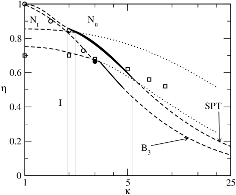
Figure 7: Phase diagram of the HR fluid. Continuous and first-order transitions are indicated by dashed and solid lines, respectively. Dotted lines indicate extension of I-N_t line into region where N_t is preempted by uniaxial nematic phase. SPT transition lines and $B_{3}$ spinodals are indicated by corresponding labels. Circles: minimisation of free-energy functional in $B_{3}$ theory, giving first-order (filled circles) or second-order (open circles) transitions. Open squares: simulation results for the isotropic-to-nematic transition.

It is also apparent from Fig. 7 that the I-N_u transition predicted by the new theory for high values of $\kappa$ occurs at packing fractions below those predicted by SPT. In the Onsager limit, the reduced transition density $\rho_{r}=\rho^{*}L^{2}$ for the I-N_u transition can be calculated within the third virial-coefficient approximation [see Eqn. (47) of the Appendix]. This reduced density depends on the coefficient $\tau^{*}$ defined in Eqn. (48), which can be calculated by extrapolating the data for $\tau(\kappa)$ obtained from simulations. These data, shown in Fig. 8 for high values of $\kappa$, are fitted very accurately by means of a straight line that intersects the vertical axis at $\tau^{*}\approx 0.314$. Inserting this value in (47), we obtain $\rho_{r}^{\rm{B_{3}}}=3.15$, which is less than the SPT result $\rho_{r}^{\rm{SPT}}=4.71$ and much less than the MC simulation value, which has been estimated to be between 7 and 7.5 Frenkel1 . This disagreement is probably due to the poorly convergent character of the virial series. As already pointed out, the fourth and fifth virial coefficients are negative in this limit, so the proper inclusion of higher-order virial coefficients is necessary in order to obtain an accurate approximation for the I-N transition densities.

Another interesting aspect of the phase diagram is the failure of the new theory to reproduce the transition from the isotropic to the nematic phase in the range of large aspect ratios explored by our simulations. Note that, as will be discussed later, the simulations cannot reach any definite conclusion as to the real nature (whether tetratic or uniaxial) of the nematic phase, especially for large aspect ratio. The fact that the isotropic-to-nematic transition line $\eta(\kappa)$ obtained from simulations in the range $\kappa=1-9$ is a smoothly decreasing monotonic curve and that this line is quite close to the spinodal line for the I-N_t transition obtained from the new theory in the same range of aspect ratios, may be indicating that the stability of the uniaxial phase is largely overestimated by the new theory, but that tetratic ordering is relatively well reproduced. This is simply a hypothesis not based on any real evidence.

Figure 8: The coefficient $\tau(\kappa)$ [see Eq. (48)] as a function of $\kappa$ for a discrete set of $\kappa$’s (open circles) calculated via Monte-Carlo integration. The straight line calculated from mean square approximation intersects the ordinate at the value indicated in the figure.

III.4 Further results

In order to appreciate more deeply the differences between the SPT and the new theory, we now compare the EOS for the isotropic and orientationally ordered phases and the behaviour of the order parameters, $q_{1},q_{2}$, with packing fraction. The latter are defined by

$$q_{i}=\int d\phi\cos{\left(2i\phi\right)}h(\phi),\hskip 19.91684pti=1,2$$ (23)

with $q_{1}$ the uniaxial order parameter and $q_{2}$ the tetratic order parameter. The comparison is done in Figs. 9(a-c) for the case $\kappa=3$ and in Figs. 10 (a-c) for $\kappa=9$. Also, the MC simulation results are shown. In the case of the EOS, both theories severely overestimate the pressure in the nematic regime when $\kappa=3$; however, the transition point, as mentioned previously, is much better reproduced when three-body correlations are included in the theory. For the longer particles the pressures are better reproduced, but the location and nature of the transition from the isotropic to the nematic phase are not correct; as already mentioned, if the uniaxial nematic phase is not taken into account, three-body correlations seem to be very important in promoting tetratic order in the isotropic phase. These correlations alone, when higher-order correlations are not considered, probably overemphasise the relative stability of the uniaxial nematic phase with respect to the tetratic phase in the case of long particles, and cause a premature instability of the latter as particles become longer.

Comparison of the orientational distribution functions in the case $\kappa=3$ indicates again the role of three-body correlations. Fig. 10 shows the corresponding function for the uniaxial nematic phase that coexists with the tetratic (new theory) or isotropic (SPT) phase; even though the new theory predicts a much lower transition density than SPT, tetratic ordering is much more pronounced in the new theory since at this value of $\kappa$ the tetratic phase is still stable.

A point worth mentioning is the identification of the value of aspect ratio where the tetratic phase is no longer stable. The nonequilibrium macroscopic experiments by Narayan et al. Narayan find substantial tetratic correlations in cylindrical particles with aspect ratio $\kappa=12.6$. Our present simulation data are not sufficiently detailed to give conclusive results. However, data for $\kappa=7$ (not shown) and $\kappa=9$ seem to be compatible with N_t stability: the value of the uniaxial order parameter $q_{1}$ is compatible with zero in the whole density range studied. In the case $\kappa=9$ [Fig. 10(b)], however, there seems to be some tendency in the uniaxial order parameter to increase from zero.

Nevertheless, it is very difficult within our present analysis, to settle this question. It is in fact difficult to distinguish between the N_t and N_u nematic phases, since the latter exhibits substantial tetratic correlations even for the longer particles considered ($\kappa=9$). Before further work is undertaken, all we can say conclusively from the simulation results is that at some packing fraction the isotropic phase begins to display substantial tetratic order in a rather abrupt manner; whether this order corresponds to uniaxial or strictly tetratic nematic phases is a matter that would require more simulation work using e.g. larger systems. Our limited study is only intended to provide approximate phase boundaries for systems of particles with various aspect ratios (note that previous simulation work on this and related systems Frenkel ; Frenkel1 ; Donev were more detailed, but restricted to a particular aspect ratio).

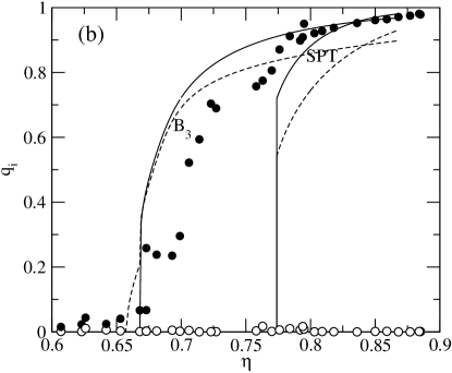
Figure 9: Results from the SPT, the present model and computer simulation for HR fluid with $\kappa=3$. (a) equation of state resulting from SPT (dashed line), our proposal (solid line) and MC simulation results (filled circles). The arrow indicates the packing fraction of the I-N transition as estimated by simulation, while the filled square indicates the location of the I-N bifurcation point predicted by the present model; (b) behaviour of the uniaxial (solid line) and tetratic (dashed line) order parameters with packing fraction. Results from SPT and our model are indicated by the corresponding label. Symbols are simulation results for the order parameters (open symbols: uniaxial, filled symbols: tetratic); (c) orientational distribution functions at the coexistence packing fraction for the uniaxial nematic phase, from SPT (dashed line) and the present model (solid line).

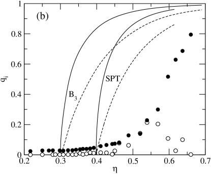
Figure 10: Same as in Fig. 9 but for $\kappa=9$. In (c) are shown the orientational distribution functions calculated at packing fractions separated from the bifurcation packing fraction a relative distance ($\Delta=0.01467$) equal to that between the isotropic and nematic coexisting packing fractions for $\kappa=3$.

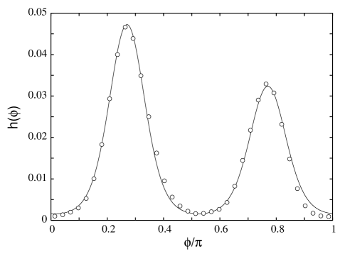
Figure 11: Orientational distribution function $h(\phi)$ from simulation for the case $\kappa=9$ and packing fraction $\eta=0.618$. Symbols: simulation data. Line: best fit to Eqn. (49). Resulting values for the order parameters are $q_{1}=0.153$ and $q_{2}=0.628$.

III.5 Dependence on EOS adopted

It should be noted that the packing fraction values of the I-N_u,t phase transitions depend sensitively on the approximation used for the EOS of the HR fluid. This can be easily shown if we approximate the third virial coefficient as a function of the second virial coefficient using the relations

$$\gamma=b_{2},\quad\beta\gamma^{2}=b_{3}-\alpha b_{2},$$ (24)

which can be easily obtained from (1) and (2) and are only valid for the isotropic fluid. From (24) we obtain

$$b_{3}=\alpha b_{2}+\beta b_{2}^{2},$$ (25)

which can be used as an approximation of the third virial coefficient of the nematic fluid. Thus, inserting the above expression in Eq. (9), and carrying out the bifurcation analysis described in Section IIC, we arrive at

$$\Delta\varphi_{k}\approx\frac{h_{k}^{2}}{4}\left[1-\Psi(y)b_{2}^{(k,k,0)}\right],\quad k=1,2$$ (26)

$$\Psi(y)=y+\left[\alpha-2+2\beta\frac{(\kappa+1)^{2}}{\pi\kappa}\right]\theta(y),$$ (27)

for the second order expansion of the free-energy difference between the I and N phases at the bifurcation point; here the subindex $k=1,2$ labels the N_u and N_t phases, respectively. Solving equation $\Delta\varphi_{k}=0$ for $\eta(\kappa)$, we find the spinodals shown in Fig. 12 for different values of $(\alpha,\beta)$ corresponding to those of SPT, Boublik’s proposal, and our proposal for the EOS of the isotropic fluid. In the same figure the spinodal line resulting from the EOS with the exact third virial coefficient is also plotted. Comparing the latter with those obtained from the different approximations embodied in (25), we conclude that the location of the I-N_u tricritical point changes only if one uses the exact three-body correlations. The reason for this behavior can be elucidated from Eqn. (26): the values of $(\eta^{*},\kappa^{*})$ calculated from $\Delta\varphi_{1}=\Delta\varphi_{2}=0$ gives us $\kappa^{*}=(3+\sqrt{5})/2$, independent on the choice of $(\alpha,\beta)$ as the function $\Psi(y)$ does not depends on $k$.

Figure 12: Spinodals of the transitions between the isotropic and orientational ordered phases. From top to bottom are shown the results from the SPT, the EOS with the approximated $b_{3}$ (the Boublik, and our proposal), and from the EOS with the exact $b_{3}$. The dotted lines represent the position of the tricritical points common to all the approximations and that corresponding to the exact $B_{3}$. Also are shown the simulation results.

IV Conclusions

The main results presented in this article can be summarized as follows. (i) The inclusion of many- (higher-than-two) body correlations in two-dimensional systems of hard anisotropic bodies is of crucial importance in order to adequately describe the phase behavior of these systems. In two-dimensions two-body interactions are not enough to make quantitative predictions of their phase behavior, a crucial difference with respect to three-dimensional systems. This conclusion is supported by simulation results. ii) We have proposed an EOS and a corresponding free energy density functional for fluids of hard rectangles that incorporates three-body correlations. While predicting pressures for the isotropic and nematic fluids which are too high when compared with simulation values, the theory gives values for the coexistence densities of the I-N_t transition that compare fairly well with the simulation results for small values of $\kappa$. A shortcoming of the theory is that the third virial coefficient, which is incorporated exactly, has to be evaluated numerically beforehand. This is a practical, not fundamental, limitation of the theory, which can be circumvented in all cases (i.e. for all different particle geometries in two dimensions).

A striking prediction of the theory is the stability of a tetratic phase, in good quantitative agreement with simulations for low particle aspect ratio. We conclude from this that the four-fold correlations present in this phase are basically taken care of by our third-virial coefficient based theory, but not by the usual scaled-particle theory, which incorporates only two-body correlations. More at variance with simulation results is the case of high aspect ratios. In this regime the stability of the uniaxial nematic phase is overestimated with respect to the isotropic fluid.

As a final comment, we must say that no attention has been paid to non-uniform phases (smectic, columnar or solid) in the present work. Previous studies by our group Martinez-Raton , based on a density-functional theory which recovers SPT in the limit of spatially uniform phases and combines Onsager and fundamental-measure theories, indicate that the tetratic phase is preempted (in the sense of bifurcation theory, i.e. spinodal lines) by a spatially ordered phase. Inclusion of three-body correlations could severely affect this result since these correlations may affect both phases differently. In fact, simulations available so far support the conclusion that the tetratic phase may be stabilised prior to crystallisation. However, even in the case that it were possible to construct a density functional, suitable for such non-uniform phases, and incorporating three-body correlations, the effort involved in the minimization with respect to the full density profile $\rho({\bf r},\phi)$ would be rather huge. Work along this avenue is now in progress in our group.

V Appendix

V.1 Bifurcation analysis

In this section we introduce the formalism that allowed us to calculate the spinodal instabilities and the order of the phase transitions between the isotropic and orientational ordered phases. This formalism is quite general, in the sense that it is independent of the geometry of particles, and includes two- and three-particle correlations. As usual, the analysis starts from an order-parameter expansion of the free-energy difference ($\Delta\varphi$) between the bifurcated (orientationally ordered) and the parent (isotropic) phases about the bifurcation point, and then the evaluation of the inverse isothermal compressibility ($\varkappa^{-1}$) of the bifurcated phase at the same point. The existence of a tricritical point, at which the order of the transition changes from second to first order, is predicted from the first change of sign (from positive to negative) of $\Delta\varphi$ or $\varkappa^{-1}$. The starting point of the bifurcation analysis is to assume that the orientational distribution function near the I-N bifurcation point can be approximated as a Fourier series in small amplitudes $h_{k}\sim\epsilon^{k}$ (where $\epsilon$ is an small parameter), truncated at second order, i.e.

$$h(\phi)\approx\frac{1}{\pi}\left(1+h_{1}\cos 2\phi+h_{2}\cos 4\phi\right).$$ (28)

Inserting this expression into (9) and (18), we obtain the difference between the nematic and isotropic free energies per particle as

$$\Delta\varphi\equiv\varphi_{\rm{N}}-\varphi_{\rm{I}}\approx Ah_{1}^{2}+Ch_{1}^{2}h_{2}+Dh_{2}^{2}+Eh_{1}^{4},$$ (29)

where the coefficients $A,C,D,E$ have the form

$$A = \frac{1}{4}\left[1-yb_{2}^{(1,1)}-\theta(y)\left(b_{3}^{(1,1,0)}-2b_{2}^{(1,1)}\right)\right],$$ (30)

$$C = -\frac{1}{8}\left[1+2\theta(y)b_{3}^{(1,1,2)}\right],$$ (31)

$$D = \frac{1}{4}\left[1-yb_{2}^{(2,2)}-\theta(y)\left(b_{3}^{(2,2,0)}-2b_{2}^{(2,2)}\right)\right],$$ (32)

$$E = \frac{1}{32},$$ (33)

and we have defined $y=\eta/(1-\eta)$. $\theta(y)=y-\ln(1+y)$ is the same function as in (10), but here in terms of the new variable $y$. The coefficients

$$b_{i}^{(k_{1},\dots,k_{i})} = -\frac{4}{\pi^{i}v^{i-1}}\left[\prod_{l=1}^{i}\int_{0}^{\pi}d\phi_{l}\cos 2k_{l}\phi_{l}\right]$$ (34)

$$\times {\cal K}(\phi_{1},\dots,\phi_{i}),\quad i=2,3,\quad k_{j}\in\mathbb{N},$$

have also been defined, which originate from two- ($i=2$) and three- ($i=3$) body correlations. For $i=2$ one can obtain analytic results which, for the specific case of HR, give

$$b_{2}^{(k,k)}=\frac{2}{(4k^{2}-1)\pi}\frac{\left(L+(-1)^{k}\sigma\right)^{2}}{v}$$ (35)

If we set $\theta(y)=0$ in (30)-(32) the SPT result is recovered. Minimizing the free energy difference (29) with respect to $h_{2}$, we obtain $h_{2}$ as a function of $h_{1}$ [$h_{2}=-Ch_{1}^{2}/(2D)$] which, inserted in (29), results in

$$\Delta\varphi = Ah_{1}^{2}+Bh_{1}^{4},$$ (36)

$$B = E-\frac{C^{2}}{4D}$$ (37)

where $A$ and $B$ are functions of the variable $y$. Minimizing Eq. (36) with respect to $h_{1}$, and taking into account the expansion of $y$ about its bifurcation value $y^{*}$, i.e. $y\approx y^{*}+y^{(2)}h_{1}^{2}$, we arrive at

$$\frac{\partial\Delta\varphi}{\partial h_{1}}=2h_{1}\left[A^{*}+\left(2B^{*}+A_{y}^{*}y^{(2)}\right)h_{1}^{2}\right]=0,$$ (38)

where $A_{y}$ is the first derivative of $A$ with respect to $y$, and the asterisk on $A,B$, and $A_{y}$ means that these functions are evaluated at the bifurcation point $y^{*}$. Solving (38) order by order, we obtain two equations:

$$A^{*} = 0,$$ (39)

$$y^{(2)} = -\frac{2B^{*}}{A_{y}^{*}},$$ (40)

the first one allowing to find $y^{*}$, and hence the packing fraction $\eta^{*}(\kappa)$, as a function of the particle aspect ratio $\kappa=L/\sigma$, i.e the spinodal line of the I-N phase transition. Expanding (36) about the bifurcation point, and using (39) and (40), we obtain

$$\Delta\varphi=-B^{*}h_{1}^{4},$$ (41)

which indicates that the I-N transition is of first order if $B^{*}<0$. Eqn. (41) can be written in a different, more convenient form, with use of $h_{1}^{2}=(y-y^{*})/y^{(2)}$ and Eqn. (40), which results in

$$\varphi_{\rm{N}}=\varphi_{\rm{I}}^{*}-\frac{\left(A_{y}^{*}\right)^{2}}{4B^{*}}(y-y^{*})^{2}.$$ (42)

Using the definition of the inverse isothermal compressibility, $\varkappa^{-1}=\rho\partial(\beta P)/\partial\rho$, in terms of the $y$ variable,

$$\varkappa^{-1}v=y(1+y)\frac{\partial}{\partial y}\left(y^{2}\frac{\partial\varphi}{\partial y}\right),$$ (43)

together with Eqn. (42), we find

$$\left(\varkappa^{-1}_{\rm{N}}v\right)^{*}=\left(\varkappa^{-1}_{\rm{I}}v\right)^{*}-\left(y^{*}\right)^{3}(1+y^{*})\frac{\left(A_{y}^{*}\right)^{2}}{2B^{*}},$$ (44)

where

$$\left(\varkappa_{\rm{I}}^{-1}v\right)^{*} = y^{*}\left(1+y^{*}\right)\left(1+2y^{*}b_{2}\right)$$ (45)

$$+ \frac{\left(y^{*}\right)^{3}\left(3+2y^{*}\right)}{1+y^{*}}(b_{3}-2b_{2}).$$

The existence of a tricritical point, at which the I-N transition changes from second to first order as particles change from large to small aspect ratios, can be found for a value of the aspect ratio $\kappa^{*}$ satifying $\kappa^{*}=\rm{max}\left(\kappa_{1},\kappa_{2}\right)$, where $\kappa_{j}$ ($j=1,2$) are the solutions to the equations

$$B^{*}(\kappa_{1})=0,\quad\left(\varkappa_{\rm{N}}^{-1}v\right)^{*}(\kappa_{2})=0$$ (46)

The preceding analysis with $h_{k}\neq 0$ ($k=1,2$) corresponds to the bifurcation analysis of the transition between the isotropic and the uniaxial nematic phase N_u. If $h_{1}=0,h_{2}\neq 0$, the bifurcating phase is a tetratic nematic phase N_t. To carry out the bifurcation analysis for the I-N_t transition, we can use exactly the same formalism, except that we have to make the substitutions $h_{k}\to h_{2k}$, and $b_{i}^{(k_{1},\dots,k_{i})}\to b_{i}^{(2k_{1},\dots,2k_{i})}$ in Eqns. (29)- (32).

Taking the Onsager limit $\kappa\to\infty$ in Eqn. (30) and considering that, in the asymptotic limit [see Eqn. (3)], the coefficients $b_{2}^{(1,1)}$ and $b_{3}^{(1,1,0)}$ are of order $\kappa$ and $\kappa^{2}$, respectively, the condition (39) is equivalent to solving a second-order equation with respect to the reduced density $\rho_{r}\equiv\rho^{*}L^{2}$, with the solution

$$\rho_{r}=\frac{1}{\tau^{*}}\left(\sqrt{1+3\pi\tau^{*}}-1\right),$$ (47)

where we have defined the coefficient

$$\tau^{*}=\lim_{\kappa\to\infty}\tau(\kappa),\quad\tau(\kappa)=\frac{3\pi}{2}\frac{b_{3}^{(1,1,0)}(\kappa)}{\kappa^{2}}.$$ (48)

The limit $\tau^{*}\to 0$ of Eq. (47) recovers the SPT result $\rho_{r}=3\pi/2$. Also $\rho_{r}(\tau^{*})$ as a function of $\tau^{*}$ is a monotonically decreasing function whose domain and image are $[-1/3\pi,\infty)$ and $(0,3\pi]$, respectively. Thus if $\tau^{*}>0$ ($\tau^{*}<0$), the I-N transition in a two-dimensional hard-needle fluid occurs at a reduced density in the interval $(0,3\pi/2]$ ($[3\pi/2,3\pi)$).

V.2 Calculation of $B_{3}$

The third virial coefficient $B_{3}(\{\lambda_{\tau}\})$ was obtained by MC integration using, for the orientational distribution function, the form

$$h(\phi)=C\exp{\left(\lambda_{1}\cos{2\phi}+\lambda_{2}\cos{4\phi}\right)}$$ (49)

which contains two free parameters, $\lambda_{1}$ and $\lambda_{2}$. The MC data for $B_{3}$ were obtained for each value of $\kappa$ explored and for fixed values of $\lambda_{1}$ and $\lambda_{2}$. The technique followed was a generalization of the standard method for isotropic fluids Hoover : each step involved generating angles for the three rectangles [see Eqn. (16)] and positions for two of them [the first rectangle is placed at the origin, see Eqn. (16)]. Since the $B_{3}$ coefficient involves a single irreducible cluster integral where all three rectangles overlap, the positions of the second and third rectangles were chosen within their respective excluded volumes with the first rectangle to insure overlap, and only one overlap condition (second with third rectangles) had to be checked. Angles were generated using an acceptance-rejection method according to the angular distribution function $h(\phi)$ corresponding to the values of $\lambda_{1}$ and $\lambda_{2}$ (the method was checked by computing the second virial coefficient $B_{2}$ for the isotropic case, which can be compared with the exact result, and also the third virial coefficient for some special particle orientations where this coefficient is analytic; in this case the computed values of $B_{2}$ and $B_{3}$ for high values of $\lambda_{1}$ and $\lambda_{2}=0$ tended to the correct value). A single MC step involves generating one chain of rectangles, and $1-2\times 10^{7}$ MC steps were used in the calculations for each set of values of $\lambda_{1},\lambda_{2}$.

We generated numerical values of $B_{3}$ at a collection of mesh points on a rectangular region of the $\lambda_{1}-\lambda_{2}$ plane. The extension of this region was chosen according to the values of the packing fraction. In any case it contained the origin ($\lambda_{1}=\lambda_{2}=0$) to allow for the isotropic phase. In some cases the region $[-1,1]\times[-1,1]$ did suffice; in others, higher minimum and maximum values for the parameters were needed, especially when a first-order transition was detected. The mesh interval was typically $\Delta\lambda=0.1$, with finer meshes when required. In order to use these data in a practical way, the data were fitted in two different ways. One involves constructing a polynomial $P_{N}(\lambda_{1},\lambda_{2})=\sum_{n=0}^{N}\sum_{m=0}^{n}c_{nm}\lambda_{1}^{m}\lambda_{2}^{n-m}$ by a least-square procedure. Symmetry considerations require some terms of this polynomial expansion not to appear, and the corresponding coefficients $c_{nm}$ were taken to be zero. The degree of the polynomial was typically in the range $8-10$. In the case of the I-N_t transition, which only involves $q_{2}$ (and hence $\lambda_{2}$), calculations were also done using fits to a polynomial depending only on $\lambda_{2}$ (since necessarily $\lambda_{1}=0$). Results are consistent with the previous results based on a full fitting.

For high packing fractions a fit to a function in the order parameters $(q_{1},q_{2})$ is more suitable since their values are close to one, whereas the $\lambda$ parameters grow without limit. However, the dependence of $B_{3}$ on $(q_{1},q_{2})$ is strong. We found it useful to use a combination of polynomials in the $q$’s and factors of the form $(q_{i}\pm 1)^{n}$, with $n$ a power whose value is optimized in the fit.

V.3 Minimization of the free-energy functional

The minimizations were done using a variational scheme. An important question is how accurate is the variational function (49). We can assess the quality of this function by comparing with simulation results for the distribution function $h(\phi)$. Fig. 11 shows a distribution-function histogram obtained from a constant-pressure MC simulation, over $2\times 10^{6}$ steps, of a fluid with $\kappa=5$ at pressure $P\sigma^{2}/kT=1.4$. This is clearly a nematic phase with tetratic order (whether this corresponds to a uniaxial or purely tetratic phase is a different matter; extremely long runs are probably needed to fully equilibrate the system. For the present purpose this is of no importance). A least-square fitting to the variational function gives $\lambda_{1}=0.033$, $\lambda_{2}=1.217$ ($q_{1}=0.008$, $q_{2}=0.523$), which results in the function represented in the figure. Histograms exhibiting more structured orientational order can be similarly fitted with comparable accuracy. The function (49) is therefore suitable as a variational function.

The nematic order parameters can be related to the variational parameters via Eqn. (23). There is a one-to-one correspondence between the sets $(q_{1},q_{2})$ and $(\lambda_{1},\lambda_{2})$. In our calculations the function $\varphi(q_{1},q_{2};\kappa,\eta)$ was then minimized with respect to $q_{1},q_{2}$, using a standard Newton-Raphson technique. All transitions are obtained as second-order transitions, except in the approximate interval $3\lesssim\kappa\lesssim 5$ where discontinuous transitions were found. Of course these results are consistent with those from bifurcation theory, which is otherwise better suited for the calculation of the tricritical points since it is not tied to any variational scheme. The value of the functional minimization can be better appreciated in the case of the N_t-N_u transition, which cannot easily be obtained using bifurcation theory.

The results of the minimisation using the resulting fitted function for $B_{3}$ are very sensitive to details such as mesh interval and degree of fitting polynomial. A detailed study of the whole procedure, including fine tuning of the above parameters, was therefore necessary. The accuracy of the results is sufficient to locate the phase transitions with respect to packing fraction, and to discriminate between first- and second-order phase transitions when the system is far from the tricritical points, but the exact density gap in first-order transitions (which is otherwise small) could not be obtained with the present numerical implementation.

V.4 Some details on MC simulations

Our constant-pressure MC simulations were performed on systems of $\sim 10^{3}-10^{4}$ HR particles, using rectangular cells and periodic boundary conditions. The equation of state, orientational distribution function and nematic order parameters were obtained during the course of these simulations. The simulations were run typically over $\sim 10^{7}$ MC steps for equilibration and $\sim 2\times 10^{7}$ MC steps for averaging (slow orientational dynamics, especially in the case of long particles, require longer runs than in the isotropic phase). The value of the pressure is fixed at some constant value. The average density (or packing fraction $\eta$) is obtained, which gives the equation of state $P(\eta)$.

The orientational order is obtained from the eigenvalues and eigenvectors of the order matrix, defined for a given particle configuration as

$$S_{ij}=\frac{1}{N}\sum_{k=1}^{N}\left(2\hat{n}_{i}^{k}\hat{n}_{j}^{k}-\delta_{ij}\right)$$ (50)

where $\hat{\bf n}^{k}$ is a unit vector along the long axis of the $k$th particle. These is to be averaged over MC configurations. The eigenvector associated with the largest eigenvalue gives the direction of the primary director, and this eigenvalue is the uniaxial order parameter, $q_{1}$, which can also be calculated from the average

$$q_{1}=\frac{1}{N}\sum_{k=1}^{N}\left<\cos{2\left(\phi_{k}-\phi_{0}\right)}\right>$$ (51)

where $\phi_{0}$ is the polar angle of the director (which depends on the configuration) and $\phi_{k}$ the polar angle of the particle long axis, both with respect to some fixed direction in the plane. The tetratic order parameter can now be calculated from a similar equation, with the factor 2 in the cosine substituted by 4. Also, the orientational distribution function $h(\phi)$ was calculated as a histogram, using the angle $\phi_{0}$ as the origin. From this the order parameters $q_{i}$ can also be obtained from Eqns. (23). Yet another route is provided by the asymptotic value of the orientational correlation functions. No attempt was made at calculating these functions in the present work.

The function $h(\phi)$ is always seen to have two maxima: a primary and a secondary maximum, separated by $\pi/2$; in the uniaxial nematic phase these maxima should have different heights, whereas in the tetratic phase their heights should be statistically equal. Due to many effects that affect the simulations, distinguishing these two situations is a rather delicate problem and our limited study did not allow identification of the true nature of the nematic phase. Questions such as effect of boundary conditions, system size, etc, may be of paramount importance in this analysis. For example, the rectangular periodic boundary conditions used in this work could be artificially promoting tetratic ordering in the system.

As is characteristic of two-dimensional systems with continuous symmetries, the orientationally ordered phases of the present model seem to exhibit quasi-long-range order at long distances Donev . This means, in particular, that the order parameters may show a strong system-size dependence. This point has not been considered at all, since our only aim was to establish approximate phase-stability boundaries that could serve as a test bed against which the (otherwise approximate) theories could be tested.

Finally, since this was not the aim of this work, and also due to the difficulties involved in dealing with possibly multiply degenerate structures, both periodic and nonperiodic, crystalline configurations have not been studied in any detail; however, freezing into glassy states in compression runs were observed to occur (these states were characterised by extremely low particle diffusion) at high density. These densities at quite close to those at which melting into a nematic phase from crystalline configurations are observed to occur in expansion runs (starting from crystals with various types of packing –particles perfectly aligned on a rectangular lattice, square clusters on square lattices, various random tilings, etc.) A full discussion of this issue can be found in Ref. Donev .

References

- (1) H. Schlacken, H. -J. Mogel, and P. Schiller, Mol. Phys. 93, 777 (1998).
- (2) Y. Martínez-Ratón, E. Velasco, and L. Mederos, J. Chem. Phys. 122, 064903 (2005).
- (3) K. W. Wojciechowski and D. Frenkel, Comp. Meth. Sci. Tech. 10, 235 (2004).
- (4) A. Donev, J. Burton, F. H. Stillinger, and S. Torquato, Phys. Rev. B 73, 054109 (2006).
- (5) M. Möbus, N. Karl and T. Kobayashi, J. Crys. Growth 116, 495 (1992); L. Nony, R. Bennewitz, O. Pfeiffer, E. Gnecco, A. Baratoff, E. Meyer, T. Eguchi, A. Gourdon and C. Joachin, Nanotechnology 15, S91-S96 (2004); H. Proehl, T. Dienel, R. Nitsche and T. Fritz, Phys. Rev. Lett. 93, 097403 (2004).
- (6) V. Narayan, N. Menon, and S. Ramaswamy, J. Stat. Mech. P01005 (2006)
- (7) L. Onsager, Ann. N. Y. Acad. Sci. 51, 627 (1949).
- (8) G. Tarjus, P. Viot, S. M.Ricci, and J. Talbot, Mol. Phys. 73, 773 (1991).
- (9) H. Reiss, H. L. Frisch, and J. L. Lebowitz, J. Chem. Phys. 31, 369 (1959).
- (10) M. A. Cotter and D. E. Martire, J. Chem. Phys. 52, 1902 (1970); J. Chem. Phys. 53, 4500 (1970); M. A. Cotter and D. C. Wacker, Phys. Rev. A 18, 2669 (1978).
- (11) G. Lasher, J. Chem. Phys. 53, 4141 (1970).
- (12) B. Barboy and W. Gelbart, J. Chem. Phys. 71, 3053 (1979).
- (13) A. Isihara, J. Chem. Phys. 18, 1446 (1950).
- (14) T. Kihara, Rev. Mod. Phys. 25, 831 (1953).
- (15) T. Boublik and I. Nezbeda, Coll. Czech. Chem. Comm. 51, 2301 (1986).
- (16) T. Boublik, Molec. Phys. 63, 685 (1988).
- (17) M. Rigby, Mol. Phys. 78, 21 (1993).
- (18) D. Frenkel and R. Eppenga, Phys. Rev. A 31, 1776 (1985).
- (19) F. H. Ree and W. G. J. Hoover, J. Chem Phys. 40, 939 (1964); D. Frenkel, J. Phys. Chem. 91, 4912 (1987).