Quantum Shot Noise

“The noise is the signal” was a saying of Rolf Landauer, one of the founding fathers of mesoscopic physics. What he meant is that fluctuations in time of a measurement can be a source of information that is not present in the time-averaged value. A physicist may actually delight in noise.

Noise plays a uniquely informative role in connection with the particle-wave duality. It was Albert Einstein who first realized (in 1909) that electromagnetic fluctuations are different if the energy is carried by waves or by particles. The magnitude of energy fluctuations scales linearly with the mean energy for classical waves, but it scales with the square root of the mean energy for classical particles. Since a photon is neither a classical wave nor a classical particle, the linear and square-root contributions coexist. Typically, the square-root (particle) contribution dominates at optical frequencies, while the linear (wave) contribution takes over at radio frequencies. If Newton could have measured noise, he would have been able to settle his dispute with Huygens on the corpuscular nature of light — without actually needing to observe an individual photon. Such is the power of noise.

The diagnostic property of photon noise was further developed in the 1960’s, when it was discovered that fluctuations can tell the difference between the radiation from a laser and from a black body: For a laser the wave contribution to the fluctuations is entirely absent, while it is merely small for a black body. Noise measurements are now a routine technique in quantum optics and the quantum mechanical theory of photon statistics (due to Roy Glauber) is textbook material.

Since electrons share the particle-wave duality with photons, one might expect fluctuations in the electrical current to play a similar diagnostic role. Current fluctuations due to the discreteness of the electrical charge are known as “shot noise”. Although the first observations of shot noise date from work in the 1920’s on vacuum tubes, our quantum mechanical understanding of electronic shot noise has progressed more slowly than for photons. Much of the physical information it contains has been appreciated only recently, from experiments on nanoscale conductors.Bla00

Types of electrical noise

Not all types of electrical noise are informative. The fluctuating voltage over a conductor in thermal equilibrium is just noise. It tells us only the value of the temperature $T$. To get more out of noise one has to bring the electrons out of thermal equilibrium. Before getting into that, let us say a bit more about thermal noise — also known as “Johnson-Nyquist noise” after the two physicists who first studied it in a quantitative way.

Thermal noise extends over all frequencies up to the quantum limit at $kT/h$. In a typical experiment one filters the fluctuations in a band width $\Delta f$ around some frequency $f$. Thermal noise then has an electrical power of $4kT\Delta f$, independent of $f$ (“white” noise). One can measure this noise power directly by the amount of heat that it dissipates in a cold reservoir. Alternatively, and this is how it is usually done, one measures the (spectrally filtered) voltage fluctuations themselves. Their mean squared is the product $4kTR\Delta f$ of the dissipated power and the resistance $R$.

Theoretically, it is easiest to describe electrical noise in terms of frequency-dependent current fluctuations $\delta I(f)$ in a conductor with a fixed, nonfluctuating voltage $V$ between the contacts. The equilibrium thermal noise then corresponds to $V=0$, or a short-circuited conductor. The spectral density $S$ of the noise is the mean-squared current fluctuation per unit band width:

$$S(f)=\langle\delta I(f)^{2}\rangle/\Delta f.$$ (1)

In equilibrium $S=4kTG$, independent of frequency. If a voltage $V\neq 0$ is applied over the conductor, the noise rises above that equilibrium value and becomes frequency dependent.

At low frequencies (typically below 10 kHz) the noise is dominated by time-dependent fluctuations in the conductance, arising from random motion of impurities. It is called “flicker noise”, or “$1/f$ noise” because of the characteristic frequency dependence. Its spectral density varies quadratically with the mean current $\bar{I}$. At higher frequencies the spectral density becomes frequency independent and linearly proportional to the current. These are the characteristics of shot noise.

The term “shot noise” draws an analogy between electrons and the small pellets of lead that hunters use for a single charge of a gun. The analogy is due to Walter Schottky, who predicted in 1918 that a vacuum tube would have two intrinsic sources of time-dependent current fluctuations: Noise from the thermal agitation of electrons (thermal noise) and noise from the discreteness of the electrical charge (shot noise).

In a vacuum tube, electrons are emitted by the cathode randomly and independently. Such a Poisson process has the property that the mean squared fluctuation of the number of emission events is equal to the average count. The corresponding spectral density equals $S=2e\bar{I}$. The factor of 2 appears because positive and negative frequencies contribute identically.

Measuring the unit of transferred charge

Schottky proposed to measure the value of the elementary charge from the shot noise power, perhaps more accurately than in the oil drop measurements which Robert Millikan had published a few years earlier. Later experiments showed that the accuracy is not better than a few percent, mainly because the repulsion of electrons in the space around the cathode invalidates the assumption of independent emission events.

It may happen that the granularity of the current is not the elementary charge. The mean current can not tell the difference, but the noise can: $S=2q\bar{I}$ if charge is transferred in independent units of $q$. The ratio $F=S/2e\bar{I}$, which measures the unit of transferred charge, is called the “Fano factor”, after Ugo Fano’s 1947 theory of the statistics of ionization.

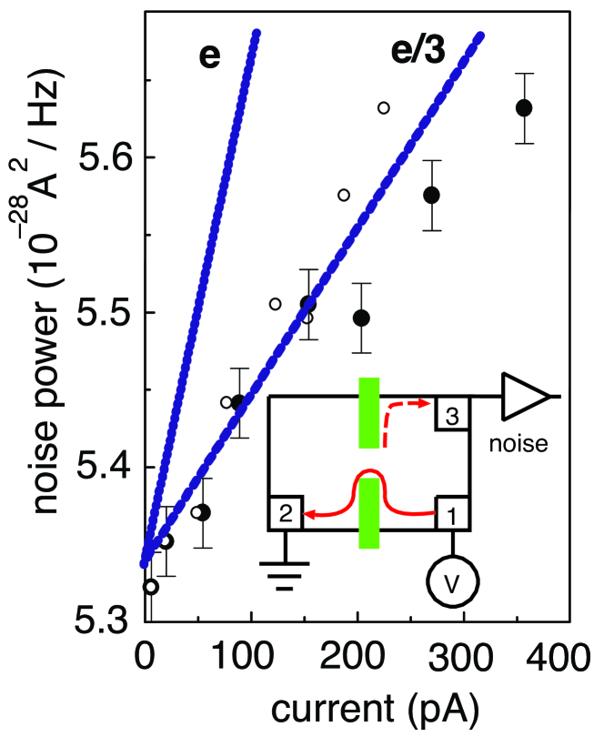
Figure 1: Current noise for tunneling across a Hall bar on the 1/3 plateau of the fractional quantum Hall effect. The slopes for $e/3$ charge quasiparticles and charge $e$ electrons are indicated. The data points with error bars (from the experiment of Saminadayar et al.Sam97 ) are the measured values at 25 mK, the open circles include a correction for finite tunnel probability. The inset shows schematically the setup of the experiment. Most of the current flows along the lower edge of the Hall bar from contact 1 to contact 2 (solid red line), but some quasiparticles tunnel to the upper edge and end up at contact 3 (dashed). The tunneling occurs predominantly at a narrow constriction, created in the Hall bar by means of a split gate electrode (shown in green). The current at contact 3 is first spectrally filtered, then amplified, and finally the mean squared fluctuation (the noise power) is measured.

A first example of $q\neq e$ is the shot noise at a tunnel junction between a normal metal and a superconductor. Charge is added to the superconductor in Cooper pairs, so one expects $q=2e$ and $F=2$. This doubling of the Poisson noise has been measured very recently.Lef02 (Earlier experiments Koz00 in a disordered system will be discussed later on.)

A second example is offered by the fractional quantum Hall effect. It is a non-trivial implication of Robert Laughlin’s theory that tunneling from one edge of a Hall bar to the opposite edge proceeds in units of a fraction $q=e/(2p+1)$ of the elementary charge.Kan94 The integer $p$ is determined by the filling fraction $p/(2p+1)$ of the lowest Landau level. Christian Glattli and collaborators of the Centre d’Études de Saclay in France and Michael Reznikov and collaborators of the Weizmann Institute in Israel independently measured $F=1/3$ in the fractional quantum Hall effectSam97 (see figure 1). More recently, the Weizmann group extended the noise measurements to $p=2$ and $p=3$. The experiments at $p=2$ show that the charge inferred from the noise may be a multiple of $e/(2p+1)$ at the lowest temperatures, as if the quasiparticles tunnel in bunches. How to explain this bunching is still unknown.

Quiet electrons

Correlations reduce the noise below the value

$$S_{\rm Poisson}=2e\bar{I}$$ (2)

expected for a Poisson process of uncorrelated current pulses of charge $q=e$. Coulomb repulsion is one source of correlations, but it is strongly screened in a metal and ineffective. The dominant source of correlations is the Pauli principle, which prevents double occupancy of an electronic state and leads to Fermi statistics in thermal equilibrium. In a vacuum tube or tunnel junction the mean occupation of a state is so small that the Pauli principle is inoperative (and Fermi statistics is indistinguishable from Boltzmann statistics), but this is not so in a metal.

An efficient way of accounting for the correlations uses Landauer’s description of electrical conduction as a transmission problem. According to the Landauer formula, the time-averaged current $\bar{I}$ equals the conductance quantum $2e^{2}/h$ (including a factor of two for spin), times the applied voltage $V$, times the sum over transmission probabilities $T_{n}$:

$$\bar{I}=\frac{2e^{2}}{h}V\sum_{n=1}^{N}T_{n}.$$ (3)

The conductor can be viewed as a parallel circuit of $N$ independent transmission channels with a channel-dependent transmission probability $T_{n}$. Formally, the $T_{n}$’s are defined as the eigenvalues of the product $t\cdot t^{\dagger}$ of the $N\times N$ transmission matrix $t$ and its Hermitian conjugate. In a one-dimensional conductor, which by definition has one channel, one would have simply $T_{1}=|t|^{2}$, with $t$ the transmission amplitude.

The number of channels $N$ is a large number in a typical metal wire. One has $N\simeq A/\lambda_{F}^{2}$ up to a numerical coefficient for a wire with cross-sectional area $A$ and Fermi wave length $\lambda_{F}$. Due to the small Fermi wave length $\lambda_{F}\simeq 1\,{\rm\AA}$ of a metal, $N$ is of order $10^{7}$ for a typical metal wire of width $1\,\mu{\rm m}$ and thickness $100\,{\rm nm}$. In a semiconductor typical values of $N$ are smaller but still $\gg 1$.

At zero temperature the noise is related to the transmission probabilities byKhl87

$$S=2e\frac{2e^{2}}{h}V\sum_{n=1}^{N}T_{n}(1-T_{n}).$$ (4)

The factor $1-T_{n}$ describes the reduction of noise due to the Pauli principle. Without it, one would have simply $S=S_{\rm Poisson}$.

The shot noise formula (4) has an instructive statistical interpretation.Lev93 Consider first a one-dimensional conductor. Electrons in a range $eV$ above the Fermi level enter the conductor at a rate $eV/h$. In a time $\tau$ the number of attempted transmissions is $\tau eV/h$. There are no fluctuations in this number at zero temperature, since each occupied state contains exactly one electron (Pauli principle). Fluctuations in the transmitted charge $Q$ arise because the transmission attempts are succesful with a probability $T_{1}$ which is different from 0 or 1. The statistics of $Q$ is binomial, just as the statistics of the number of heads when tossing a coin. The mean-squared fluctuation $\langle\delta Q^{2}\rangle$ of the charge for binomial statistics is given by

$$\langle\delta Q^{2}\rangle=e^{2}(\tau eV/h)T_{1}(1-T_{1}).$$ (5)

The relation $S=(2/\tau)\langle\delta Q^{2}\rangle$ between the mean-squared fluctuation of the current and of the transmitted charge brings us to eq. (4) for a single channel. Since fluctuations in different channels are independent, the multi-channel version is simply a sum over channels.

The quantum shot noise formula (4) has been tested experimentally in a variety of systems. The groups of Reznikov and Glattli used a quantum point contact: A narrow constriction in a two-dimensional electron gas with a quantized conductance. The quantization occurs because the transmission probabilities are either close to 0 or close to 1. Eq. (4) predicts that the shot noise should vanish when the conductance is quantized, and this was indeed observed. (The experiment was reviewed by Henk van Houten and Beenakker in Physics Today, July 1996, page 22.)

A more stringent test used a single-atom junction, obtained by the controlled breaking of a thin aluminum wire.Cro01 The junction is so narrow that the entire current is carried by only three channels ($N=3$). The transmission probabilities $T_{1},T_{2},T_{3}$ could be measured independently from the current–voltage characteristic in the superconducting state of aluminum. By inserting these three numbers (the “pin code” of the junction) into eq. (4), a theoretical prediction is obtained for the shot noise power — which turned out to be in good agreement with the measured value.

Detecting open transmission channels

The analogy between an electron emitted by a cathode and a bullet shot by a gun works well for a vacuum tube or a point contact, but seems a rather naive description of the electrical current in a disordered metal or semiconductor. There is no identifiable emission event when current flows through a metal and one might question the very existence of shot noise. Indeed, for three quarters of a century after the first vacuum tube experiments there did not exist a single measurement of shot noise in a metal. A macroscopic conductor (say, a piece of copper wire) shows thermal noise, but no shot noise.

We now understand that the basic requirement on length scale and temperature is that the length $L$ of the wire should be short compared to the inelastic electron-phonon scattering length $l_{\rm in}$, which becomes longer and longer as one lowers the temperature. For $L>l_{\rm in}$ each segment of the wire of length $l_{\rm in}$ generates independent voltage fluctuations, and the net result is that the shot noise power is reduced by a factor $l_{\rm in}/L$. Thermal fluctuations, in contrast, are not reduced by inelastic scattering (which can only help the establishment of thermal equilibrium). This explains why only thermal noise could be observed in macroscopic conductors. (As an aside, we mention that inelastic electron-electron scattering, which persists until much lower temperatures than electron-phonon scattering, does not suppress shot noise, but rather enhances the noise power a little bit.Nag95 )

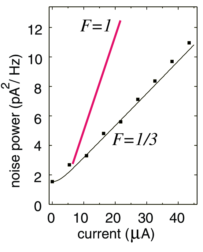
Figure 2: Sub-Poissonian shot noise in a disordered gold wire (dimensions 940 nm $\times$ 100 nm). At low currents the noise saturates at the level set by the temperature of 0.3 K. [Adapted from M. Henny et al.Ste96 ]

Early experimentsLie94 on mesoscopic semiconducting wires observed the linear relation between noise power and current that is the signature of shot noise, but could not accurately measure the slope. The first quantitative measurement was performed in a thin-film silver wire by Andrew Steinbach and John Martinis at the US National Institute of Standards and Technology in Boulder, collaborating with Michel Devoret from Saclay.Ste96

The data shown in figure 2 (from a more recent experiment) presents a puzzle: If we calculate the slope, we find a Fano factor of 1/3 rather than 1. Surely there are no fractional charges in a normal metal conductor?

A one-third Fano factor in a disordered conductor had actually been predicted prior to the experiments. The prediction was made independently by Kirill Nagaev of the Institute of Radio-Engineering and Electronics in Moscow and by one of the authors (Beenakker) with Markus Büttiker of the University of Geneva.Bee92 To understand the experimental finding we recall the general shot noise formula (4), which tells us that sub-Poissonian noise ($F<1$) occurs when some channels are not weakly transmitted. These socalled “open channels” have $T_{n}$ close to 1 and therefore contribute less to the noise than expected for a Poisson process.

The appearance of open channels in a disordered conductor is surprising. Oleg Dorokhov of the Landau Institute in Moscow first noticed the existence of open channels in 1984, but the physical implications were only understood some years later, notably through the work of Yoseph Imry of the Weizmann Institute. The one-third Fano factor follows directly from the probability distribution of the transmission eigenvalues, see figure 3.

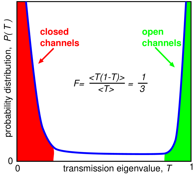
Figure 3: Bimodal probability distribution of the transmission eigenvalues, with a peak at 0 (closed channels) and a peak at 1 (open channels). The functional form of the distribution (derived by Dorokhov) is $P(T)\propto T^{-1}(1-T)^{-1/2}$, with a mean-free-path dependent cutoff at exponentially small $T$. The one-third Fano factor follows directly from the ratio $\int T^{2}P(T)dT/\int TP(T)dT=2/3$. The cutoff affects only the normalization of $P(T)$ and drops out of this ratio, which takes on a universal value.

We conclude this section by referring to the experimental demonstrationsKoz00 of the interplay between the doubling of shot noise due to superconductivity and the 1/3 reduction due to open channels, resulting in a 2/3 Fano factor. These experiments show that open channels are a general and universal property of disordered systems.

Distinguishing particles from waves

So far we have encountered two diagnostic properties of shot noise: It measures the unit of transferred charge in a tunnel junction and it detects open transmission channels in a disordered wire. A third diagnostic appears in semiconductor microcavities known as quantum dots or electron billiards. These are small confined regions in a two-dimensional electron gas, free of disorder, with two narrow openings through which a current is passed. If the shape of the confining potential is sufficiently irregular (which it typically is), the classical dynamics is chaotic and one can search for traces of this chaos in the quantum mechanical properties. This is the field of quantum chaos.

Here is the third diagnostic: Shot noise in an electron billiard can distinguish deterministic scattering, characteristic for particles, from stochastic scattering, characteristic for waves. Particle dynamics is deterministic: A given initial position and momentum fixes the entire trajectory. In particular, it fixes whether the particle will be transmitted or reflected, so the scattering is noiseless on all time scales. Wave dynamics is stochastic: The quantum uncertainty in position and momentum introduces a probabilistic element into the dynamics, so it becomes noisy on sufficiently long time scales.

The suppression of shot noise in a conductor with deterministic scattering was predicted many years agoBee91 from this qualitative argument. A better understanding, and a quantitative description, of how shot noise measures the transition from particle to wave dynamics was developed recently by Oded Agam of the Hebrew University in Jerusalem, Igor Aleiner of the State University of New York in Stony Brook, and Anatoly Larkin of the University of Minnesota in Minneapolis.Aga00 The key concept is the Ehrenfest time, which is the characteristic time scale of quantum chaos.

In classical chaos, the trajectories are highly sensitive to small changes in the initial conditions (although uniquely determined by them). A change $\delta x(0)$ in the initial coordinate is amplified exponentially in time: $\delta x(t)=\delta x(0)e^{\alpha t}$. Quantum mechanics introduces an uncertainty in $\delta x(0)$ of the order of the Fermi wave length $\lambda_{F}$. One can think of $\delta x(0)$ as the initial size of a wave packet. The wave packet spreads over the entire billiard (of size $L$) when $\delta x(t)=L$. The time

$$\tau_{E}=\alpha^{-1}\ln(L/\lambda_{F})$$ (6)

at which this happens is called the Ehrenfest time.

The name refers to Paul Ehrenfest’s 1927 principle that quantum mechanical wave packets follow classical, deterministic, equations of motion. In quantum chaos this correspondence principle loses its meaning (and the dynamics becomes stochastic) on time scales greater than $\tau_{E}$. An electron entering the billiard through one of the openings dwells inside on average for a time $\tau_{\rm dwell}$ before exiting again. Whether the dynamics is deterministic or stochastic depends, therefore, on the ratio $\tau_{\rm dwell}/\tau_{E}$. The theoretical expectation for the dependence of the Fano factor on this ratio is plotted in figure 4.

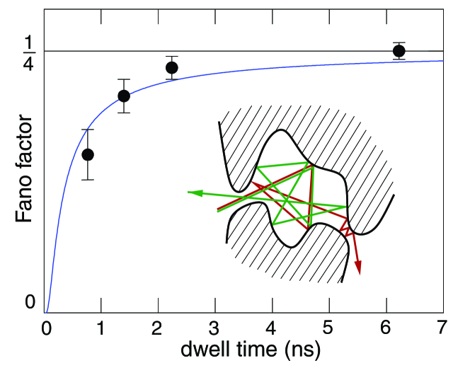
Figure 4: Dependence of the Fano factor $F$ of an electron billiard on the average time $\tau_{\rm dwell}$ that an electron dwells inside. The data points with error bars are measured in a two-dimensional electron gas, the solid curve is the theoretical prediction $F=\frac{1}{4}\exp(-\tau_{E}/\tau_{\rm dwell})$ for the transition from stochastic to deterministic scattering (with Ehrenfest time $\tau_{E}=0.27\,{\rm ns}$ as a fit parameter). The inset shows graphically the sensitivity to initial conditions of the chaotic dynamics. (Adapted from ref. Aga00, , with experimental data from ref. Obe02, .)

An experimental search for the suppression of shot noise by deterministic scattering was carried out at the University of Basel by Stefan Oberholzer, Eugene Sukhorukov, and one of the authors (Schönenberger).Obe02 The data is included in figure 4. An electron billiard (area $A\approx 53\,\mu{\rm m}^{2}$) with two openings of variable width was created in a two-dimensional electron gas by means of gate electrodes. The dwell time (given by $\tau_{\rm dwell}=m^{\ast}A/\hbar N$, with $m^{\ast}$ the electron effective mass) was varied by changing the number of modes $N$ transmitted through each of the openings.

The Fano factor has the value $1/4$ for long dwell times, as expected for stochastic chaotic scattering. The $1/4$ Fano factor for a chaotic billiard has the same origin as the $1/3$ Fano factor for a disordered wire, explained in figure 3. (The different number results because of a larger fraction of open channels in a billiard geometry.) The reduction of the Fano factor below $1/4$ at shorter dwell times fits the exponential function $F=\frac{1}{4}\exp(-\tau_{E}/\tau_{\rm dwell})$ of Agam, Aleiner, and Larkin. However, the accuracy and range of the experimental data is not yet sufficient to distinguish this prediction from competing theories (notably the rational function $F=\frac{1}{4}(1+\tau_{E}/\tau_{\rm dwell})^{-1}$ predicted by Sukhorukov for short-range impurity scattering).

Entanglement detector

The fourth and final diagnostic property that we would like to discuss, shot noise as detector of entanglement, was proposed by Sukhorukov with Guido Burkard and Daniel Loss from the University of Basel.Bur00

A multi-particle state is entangled if it can not be factorized into a product of single-particle states. Entanglement is the primary resource in quantum computing, in the sense that any speed-up relative to a classical computer vanishes if the entanglement is lost, typically through interaction with the environment (see the article by John Preskill, Physics Today, July 1999, page 24). Electron-electron interactions lead quite naturally to an entangled state, but in order to make use of the entanglement in a computation one would need to be able to spatially separate the electrons without destroying the entanglement. In this respect the situation in the solid state is opposite to that in quantum optics, where the production of entangled photons is a complex operation, while their spatial separation is easy.

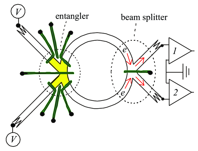
Figure 5: Proposal for production and detection of a spin-entangled electron pair. The double quantum dot (shown in yellow) is defined by gate electrodes (green) on a two-dimensional electron gas. The two voltage sources at the far left inject one electron in each dot, resulting in an entangled spin-singlet ground state. A voltage pulse on the gates then forces the two electrons to enter opposite arms of the ring. Scattering of the electron pair by a tunnel barrier (red arrows) creates shot noise in each of the two outgoing leads at the far right, which is measured by a pair of amplifiers (1,2). The observation of a positive correlation between the current fluctuations at 1 and 2 is a signature of the entangled spin-singlet state. (Figure courtesy of L.P. Kouwenhoven and A.F. Morpurgo, Delft University of Technology.)

One road towards a solid-state based quantum computer has as its building block a pair of quantum dots, each containing a single electron. The strong Coulomb repulsion keeps the electrons separate, as desired. In the ground state the two spins are entangled in the singlet state $|\!\uparrow\rangle|\!\downarrow\rangle-|\!\downarrow\rangle|\!\uparrow\rangle$. This state may already have been realized experimentally,Hol02 but how can one tell? Noise has the answer.

To appreciate this we contrast “quiet electrons” with “noisy photons”. We recall that Fermi statistics causes the electron noise to be smaller than the Poisson value (2) expected for classical particles. For photons the noise is bigger than the Poisson value because of Bose statistics. What distinghuishes the two is whether the wave function is symmetric or antisymmetric under exchange of particle coordinates. A symmetric wave function causes the particles to bunch together, increasing the noise, while an antisymmetric wave function has the opposite effect (“antibunching”). The key point here is that only the symmetry of the spatial part of the wave function matters for the noise. Although the full many-body electron wavefunction, including the spin degrees of freedom, is always antisymmetric, the spatial part is not so constrained. In particular, electrons in the spin-singlet state have a symmetric wave function with respect to exchange of coordinates, and will therefore bunch together like photons.

The experiment proposed by the Basel theorists is sketched in figure 5. The two building blocks are the entangler and the beam splitter. The beam splitter is used to perform the electronic analogue of the optical Hanbury Brown and Twiss experiment.Hen99 In such an experiment one measures the cross-correlation of the current fluctuations in the two arms of a beam splitter. Without entanglement, the correlation is positive for photons (bunching) and negative for electrons (antibunching). The observation of a positive correlation for electrons is a signature of the entangled spin-singlet state. In a statistical sense, the entanglement makes the electrons behave as photons.

An alternative to the proposal shown in figure 5 is to start from Cooper pairs in a superconductor, which are also in a spin-singlet state.Bur00 The Cooper pairs can be extracted from the superconductor and injected into a normal metal by application of a voltage over a tunnel barrier at the metal–superconductor interface.

Experimental realization of one these theoretical proposals would open up a new chapter in the use of noise as a probe of quantum mechanical properties of electrons. Although this range of applications is still in its infancy, the field as a whole has progressed far enough to prove Landauer right: There is a signal in the noise.

References

- (1) For an overview of the entire literature on quantum shot noise, we refer to: Ya.M. Blanter and M. Büttiker, Phys. Rep. 336, 1 (2000).
- (2) F. Lefloch, C. Hoffmann, M. Sanquer, and D. Quirion, Phys. Rev. Lett. 90, 067002 (2003).
- (3) A.A. Kozhevnikov, R.J. Schoelkopf, and D.E. Prober, Phys. Rev. Lett. 84, 3398 (2000); X. Jehl, M. Sanquer, R. Calemczuk, and D. Mailly, Nature 405, 50 (2000).
- (4) C.L. Kane and M.P.A. Fisher, Phys. Rev. Lett. 72, 724 (1994).
- (5) L. Saminadayar, D.C. Glattli, Y. Jin, and B. Etienne, Phys. Rev. Lett. 79, 2526 (1997); R. de-Picciotto, M. Reznikov, M. Heiblum, V. Umansky, G. Bunin, and D. Mahalu, Nature 389, 162 (1997); M. Reznikov, R. de-Picciotto, T.G. Griffiths, M. Heiblum, and V. Umansky, Nature 399, 238 (1999); Y. Chung, M. Heiblum, and V. Umansky, preprint.
- (6) V.A. Khlus, Sov. Phys. JETP 66, 1243 (1987); G.B. Lesovik, JETP Lett. 49, 592 (1989); M. Büttiker, Phys. Rev. Lett. 65, 2901 (1990).
- (7) L.S. Levitov and G.B. Lesovik, JETP Lett. 58, 230 (1993).
- (8) R. Cron, M. F. Goffman, D. Esteve, and C. Urbina, Phys. Rev. Lett. 86, 4104 (2001).
- (9) K.E. Nagaev, Phys. Rev. B 52, 4740 (1995); V.I. Kozub and A.M. Rudin, Phys. Rev. B 52, 7853 (1995).
- (10) F. Liefrink, J.I. Dijkhuis, M.J.M. de Jong, L.W. Molenkamp, and H. van Houten, Phys. Rev. B 49, 14066 (1994).
- (11) A.H. Steinbach, J.M. Martinis, and M.H. Devoret, Phys. Rev. Lett. 76, 3806 (1996). More recent experiments include R.J. Schoelkopf, P.J. Burke, A.A. Kozhevnikov, D.E. Prober, and M.J. Rooks, Phys. Rev. Lett. 78, 3370 (1997); M. Henny, S. Oberholzer, C. Strunk, and C. Schönenberger, Phys. Rev. B 59, 2871 (1999).
- (12) C.W.J. Beenakker and M. Büttiker, Phys. Rev. B 46, 1889 (1992); K.E. Nagaev, Phys. Lett. A 169, 103 (1992).
- (13) C.W.J. Beenakker and H. van Houten, Phys. Rev. B 43, 12066 (1991).
- (14) O. Agam, I. Aleiner, and A. Larkin, Phys. Rev. Lett. 85, 3153 (2000).
- (15) S. Oberholzer, E.V. Sukhorukov, and C. Schönenberger, Nature 415, 765 (2002).
- (16) G. Burkard, D. Loss, and E.V. Sukhorukov, Phys. Rev. B 61, 16303 (2000). The alternative entangler using Cooper pairs is described in: M.-S. Choi, C. Bruder, and D. Loss, Phys. Rev. B 62, 13569 (2000); G.B. Lesovik, T. Martin, and G. Blatter, Eur. Phys. J. B 24, 287 (2001).
- (17) A.W. Holleitner, R.H. Blick, A.K. Hüttel, K. Eberl, and J.P. Kotthaus, Science 297, 70 (2002); W.G. van der Wiel, S. De Franceschi, J.M. Elzerman, T. Fujisawa, S. Tarucha, and L.P. Kouwenhoven, Rev. Mod. Phys. 75, 1 (2003).
- (18) M. Henny, S. Oberholzer, C. Strunk, T. Heinzel, K. Ensslin, M. Holland, and C. Schönenberger, Science 284, 296 (1999); W.D. Oliver, J. Kim, R.C. Liu, and Y. Yamamoto, Science 284, 299 (1999).