Surface superconducting states in a polycrystalline MgB₂ sample

Abstract

We report results of dc magnetic and ac linear low-frequency study of a polycrystalline MgB₂ sample. AC susceptibility measurements at low frequencies, performed under dc fields parallel to the sample surface, provide a clear evidence for surface superconducting states in MgB₂.

Nucleation of superconducting (SC) phase in the surface sheath under a dc magnetic field parallel to the surface was predicted by Saint-James and de Gennes more than 40 years ago PG . This prediction was made in the frame of the one-band isotropic Ginzburg-Landau (GL) model and experimental confirmations of this prediction were described in various publications (see, for example, ROLL ). The discovery of superconductivity in two-band anisotropic MgB₂ raised a question about the existence of surface superconducting states (SSS) in this material. Transport measurements under dc fields indicate that the onset of the SC transition occurs above the second critical field, $H_{c2}$ determined from specific heat data LYARD ; RYDH .

In this work we present the experimental results of dc and ac measurements on polycrystalline MgB₂ sample. It appears that large losses with a maximum at certain temperature dependent dc field and complete diamagnetic screening of an ac field are observed in magnetic fields when the dc magnetic moment is very small. This is clear evidence for the existence of SSS in this material.

The MgB₂ sample with $T_{c}=37.5$ K and $\Delta T_{c}=0.5$ K was prepared using the Hot Isostatic Pressing method PASHA1 . The sample dimensions are $10\times 3\times 1$ mm³. DC magnetization curves were measured by a SQUID magnetometer. ac susceptibility was measured by the pick-up coils method SH in the frequency range $5\leq\omega/2\pi\leq 1065$ Hz. An ac ”home-made” setup was adapted to a commercial SQUID magnetometer and its block diagram was published elsewhere LEV2 . The experiments were carried out as follows. The sample was cooled down in zero magnetic field, then both dc ($H_{0}$) and ac magnetic field with amplitude $h_{0}$ were applied and the amplitude and phase of ac response was measured. Both $H_{0}$ and $h_{0}$ were parallel to the longest sample axis.

Assuming that in zero dc field there is a complete screening of ac field without any losses, one could measure the absolute value of ac susceptibility, $\chi^{\prime}$ and $\chi^{\prime\prime}$, as a function of external parameters, such as dc field, frequency, and temperature. At low ac amplitudes the response is linear and does not depend on $h_{0}$ as shown in the inset (a) to Fig. 1b, where the $\chi^{\prime\prime}$ at $\omega/2\pi=1000$ Hz, $H_{0}=4.3$ kOe, and $T=36$ K is plotted as a function of $h_{0}$. Fig. 1a shows magnetization loop $M(H_{0})$ at $T=34$ K (upper inset) and the high field $M(H_{0})$ data in an extended scale (main panel), where the irreversibility field, $H_{irr}$ and $H_{c2}$ are indicated. The lower inset of Fig. 1a presents $H_{irr}(T)$ curve. These results are consistent with the data reported previously (see, for example, CAN and references therein).

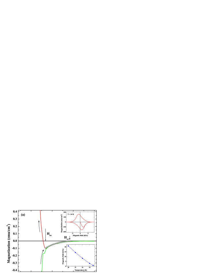
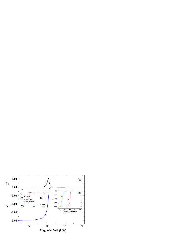
Figure 1: (Color online) (a) Magnetization curve, $M(H_{0})$, in high magnetic fields. $\nabla$ - theoretical calculations for two-band model. Upper inset - magnetization loop after ZFC at $T=34$ K. Lower inset - $H_{irr}(T)$. (b) Magnetic field dependence of $\chi^{\prime\prime}$ and $\chi^{\prime}$ at $\omega/2\pi=1065$ Hz in high magnetic fields. Insets: (a) $\chi^{\prime\prime}(h_{0})$ dependence at $T=36$ K; (b) $\chi_{dc}\equiv M(H_{0})/H_{0}$ for the virgin curve, and $\chi^{\prime}(H_{0})$ in whole range of dc field.

The inset (b) in Fig. 1b shows dc and ac susceptibility measured at 34 K as a function of dc field. It is evident that the $\chi_{dc}\equiv M(H_{0})/H_{0}$ is already very small at 5 kOe, whereas the $\chi^{\prime}$ becomes zero only above 12 kOe. The dc field dependence of $\chi^{\prime}$ and of $\chi^{\prime\prime}$ is shown in Fig. 1b (main panel). Here again, the $\chi^{\prime}$ curve exhibits ideal diamagnetism in fields much higher than 5 kOe. Note the high peak of losses at about 11 kOe, Fig. 1b, which considerably exceeds the losses both in the normal and Meissner states. A frequency dispersion of $\chi$ is also evident (see Fig. 2). All these features are typical for the ac response in SSS of low-temperature superconductors (LTS)  ROLL ; GLT . However, there is an apparent difference. In isotropic LTS these features are observed only at $H_{0}>H_{c2}$, where bulk dc magnetization is zero. In contrast, in polycrystalline MgB₂ SSS are observed below $H_{c2}$ (see Figs. 1a and 1b) and coexist with dc bulk magnetization. The dc moment in this region is reversible and small, but unambiguously has a bulk origin. In order to prove this, we applied a low-frequency shaking field with the amplitude of 2.5 Oe. We did not observe any change of the dc magnetization curve. Any possible nonzero surface current contribution to dc magnetic moment has a nonequilibrium character if the volume is in the normal state, and one could expect hysteresis and disappearance of the dc magnetization after the application of the shaking ac field. On the other hand, the ac response cannot be attributed to bulk properties. For example, at $T=34$ K and $H_{0}=10.2$ kOe $\chi^{\prime}$ at 1065 Hz is about 0.5 (the midpoint of the transition in Fig. 1b, main panel). This value is 3 orders of magnitude higher than the experimental $dM/dH_{0}$ measured under the same conditions.

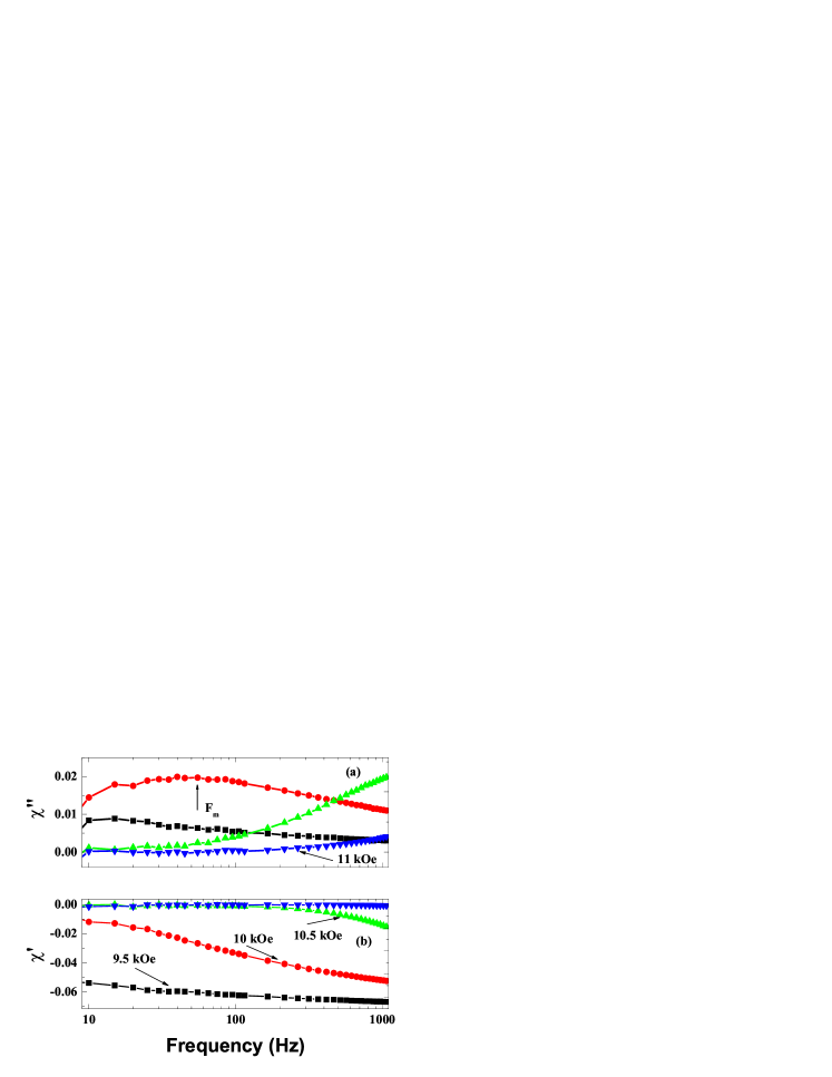
Figure 2: (Color online) Frequency dependence of $\chi^{\prime\prime}$ (a) and $\chi^{\prime}$ (b) at $T=34$ K for different magnetic fields. The symbols for the fields in both figures are identical.

The frequency dependence of $\chi^{\prime}$ and $\chi^{\prime\prime}$ at constant dc fields is shown in Fig. 2. It is clear that in some fields $\chi^{\prime}(\omega)\propto\ln(\omega)$. $\chi^{\prime\prime}$ show a maximum at $\omega/2\pi=F_{m}$ and this maximum moves with dc field as shown in Fig. 3. One may predict that, similar to the spin-glass state, the low frequency dynamics of SSS could be characterized by a broad spectrum of relaxation times with some maximum value $\tau$. Indeed, Fig. 3 shows that $F_{m}(H_{0})$ divides the frequency - magnetic field phase diagram into two parts, above and below the line, where $\omega\tau>1$ and $\omega\tau<1$, respectively.

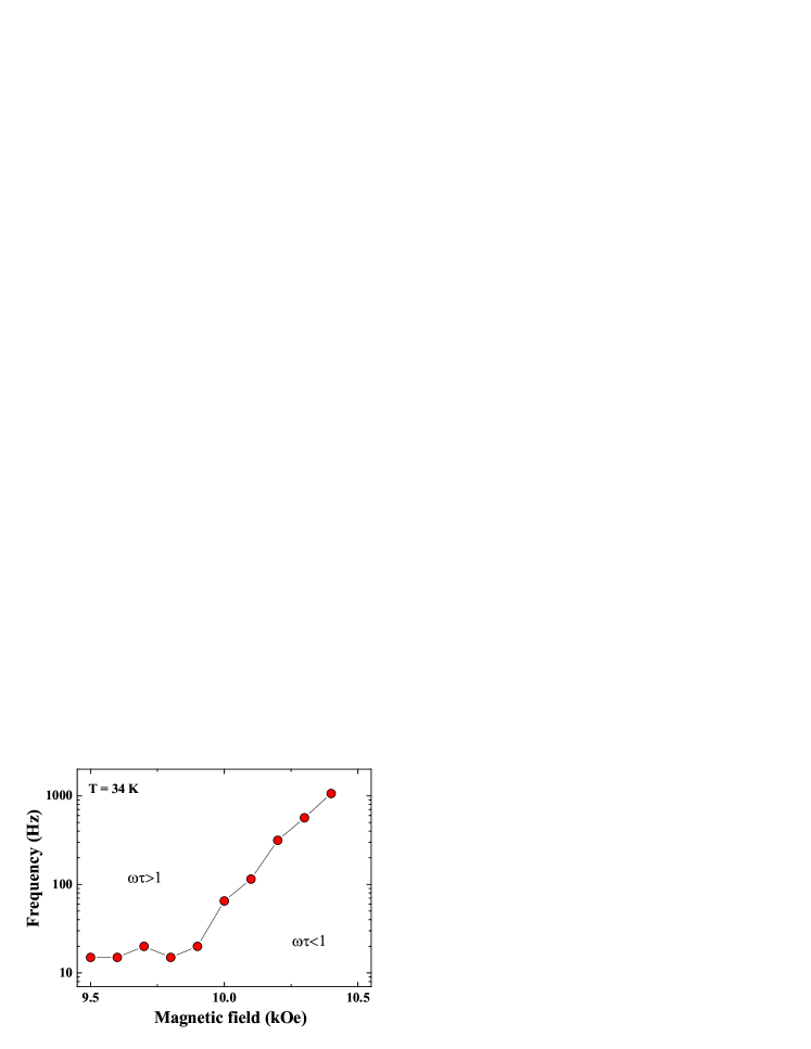
Figure 3: (Color online) Magnetic field dependence of $F_{m}$.

GL equations for two-band anisotropic superconductors were discussed in numbers of articles GUR ; ASK ; ZT and in linear approximation these take the form:

$$\mu_{sij}\Pi_{i}\Pi_{j}\Delta_{s}-\alpha_{s}(T)\Delta_{s}-\delta_{ss^{\prime}}\Delta_{s^{\prime}}=0$$ (1)

where the index $s=1$(2) corresponds to the $\sigma$($\pi$) bands, $\Pi_{j}\equiv i\nabla_{j}+2eA_{j}/\hbar c$, $\overrightarrow{A}$ - vector potential, $\Delta_{s}$ - order parameter of $s$ band, $\widehat{\mu}_{s}$ - inverse mass tensor and $\delta_{ss^{\prime}}$ is different from zero only if $s\neq s^{\prime}$. The coefficients in these equations, $\widehat{\mu}_{s}$, $\alpha_{s}(T)$ and $\delta_{ss^{\prime}}$, are given through the BCS superconducting coupling matrix $\lambda_{nm}$ and could be found in GUR ; ZT . Let us consider the superconducting slab of thickness $2D$ in a magnetic field parallel to its surface and chose the coordinate system with $x$-axis perpendicular to the surface, magnetic field along $z$-axis and the plane $x=0$ in the center of the slab. The second, $H_{c2}$, and the third critical magnetic fields, $H_{c3}$, are determined as the maximum fields for which the eigen solutions of linearized Eq. (1) with vector potential $\overrightarrow{A}(0,Hx,0)$ and appropriate boundary conditions could be found. Looking for the solution of Eq. (1) in the form:

$$\Delta_{s}=f_{s}(x)\exp(iky+ik_{z}z-i\widetilde{\mu}_{sxz}k_{z}x+i\widetilde{\mu}_{sxy}hx^{2}/2)$$ (2)

one obtains

$$\begin{array}[]{c}\frac{d^{2}f_{s}}{dx^{2}}-(\widetilde{\mu}_{syy}-\widetilde{\mu}_{sxy}^{2})h^{2}(x-x_{s})^{2}f_{s}+(\widetilde{\alpha}+g)f_{s}+\\ \widetilde{\delta}_{ss^{\prime}}f_{s^{\prime}}exp(i\phi_{s^{\prime}})=0\\ g=\frac{(\widetilde{\mu}_{yz}-\widetilde{\mu}_{xy}\widetilde{\mu}_{xz})^{2}-(\widetilde{\mu}_{zz}-\widetilde{\mu}^{2}_{xz})(\widetilde{\mu}_{yy}-\widetilde{\mu}_{xy}^{2})}{\widetilde{\mu}_{yy}-\widetilde{\mu}^{2}_{xy}}<0\\ x_{s}=k/h+\frac{\widetilde{\mu}_{yz}-\widetilde{\mu}_{xy}\widetilde{\mu}_{xz}}{\widetilde{\mu}_{yy}-\widetilde{\mu}^{2}_{xy}}k_{z}/h,\end{array}$$ (3)

with $\phi_{1}=-\phi_{2}=(\widetilde{\mu}_{1xy}-\widetilde{\mu}_{2xy})(kx-hx^{2}/2)+(\widetilde{\mu}_{1xz}-\widetilde{\mu}_{2xz})k_{z}x$, and boundary conditions $df_{s}(D)/dx=0$. Here the dimensionless variables are used: $h=2eH_{0}/\hbar c$, $\widetilde{\mu}_{sik}=\mu_{sik}/\mu_{sxx}$, $\widetilde{\alpha}_{s}=\alpha_{s}/\mu_{sxx}$, $\widetilde{\delta}_{ss^{\prime}}=\delta_{ss^{\prime}}/\mu_{sxx}$. $H_{c2}$ is determined by the maximum field for which the solution of Eqs. (3) exists at $k=k_{z}=0$ with boundary conditions $df_{s}(0)/dx=0$ and $df_{s}(D)/dx=0$ and $H_{c3}$ is determined by the solutions of this equation with $k\approx hD$, $f_{s}(0)=0$ and $df_{s}(D)/dx=0$.

At first we discuss the one-band anisotropic superconductor, $\delta_{ss^{\prime}}=0$. Equations (3) are of the same type as in the isotropic case with GL parameter $\kappa=\sqrt{\widetilde{\mu}_{yy}-\widetilde{\mu}^{2}_{xy}}$, and using the known solution PG we obtain $H_{c3}=1.695\alpha(\mu_{xx}\mu_{yy}-\mu^{2}_{xy})^{-1/2}$. $H_{c2}$ is also determined by Eq. (3) and equals to $\alpha(\mu_{xx}\mu_{yy}-\mu^{2}_{xy})^{-1/2}$ KOG . Thus the ratio $H_{c3}/H_{c2}$ for anisotropic crystals does not depend on the orientations of principal axes and is the same as for the isotropic case. For a two-band superconductor with different $\mu_{ik}$ the analytical solution hardly could be found and the numerical simulations can be successfully used. For an uniaxial crystal, $H_{c2}$ depends only on the angle $\theta$ between the $c$-axis and the direction of the dc magnetic field. In polycrystalline samples only the grains with $H_{c2}>H_{0}$ give a contribution into the equilibrium magnetic moment CLM ; BUD :

$$\begin{array}[]{c}M_{eq}(H_{0})=\int^{\pi/2}_{0}\frac{(H_{0}-H_{c2}(\theta))}{8\pi\beta_{c}\kappa^{2}}\times\\ \Theta(H_{c2}(\theta)-H_{0})\varepsilon(\theta)sin(\theta)d\theta,\end{array}$$ (4)

where function $\varepsilon(\theta)$ also takes into account the anisotropy of the vortex lattice and is equal to 1 for isotropic sample, $\beta_{c}=1.16$, and $\Theta(y)=1$ for $y>0$ and zero otherwise. For an uniaxial two-band superconductor, $\varepsilon(\theta)$ is not known yet while for the one-band superconductor it was calculated in CLM , $\varepsilon(\theta)=[\sin^{2}(\theta)+\gamma^{2}\cos^{2}(\theta)]/\gamma^{2/3}$, where the anisotropy parameter $\gamma=H_{c2}(\pi/2)/H_{c2}(0)$. Using for the coupling matrix from  RYD $\lambda_{11}=0.81$, $\lambda_{22}=0.285$, $\lambda_{12}=0.119$, $\lambda_{21}=0.091$ and $\mu_{2c}/\mu_{2a}=1.487$, $\mu_{1a}/\mu_{2a}=0.2$ ZT and varying $\mu_{1c}/\mu_{1a}$, the equilibrium magnetization near $H_{c2}$ have been calculated for different temperatures. We found that using $\mu_{ik}$ for clean limit with $\mu_{1c}/\mu_{1a}=0.048$ and $\varepsilon=1$ gives the best fit to experimental data. The result of these calculations is shown in Fig. 1a by triangles. The GL parameters obtained from this procedure are: $\kappa=18.6$, 16.1 and 13.8 for $T=34$ K, 36 K and 37 K, respectively. The GL formulae for one band isotropic superconductor with $\kappa=H_{c2}/H_{c}\sqrt{2}$, where $H_{c}$ is the thermodynamic critical field and $M_{eq}=(H_{0}-H_{c2})/8\pi\beta_{c}\kappa^{2}$, gives $\kappa=7.7$, 7.8, and 13.9 for the same temperatures. At $T=36$ K and $H_{0}=3$ kOe, $M_{eq}$ from this formula is 1.81 emu/cm³, whereas the experimental value is significantly smaller, 0.11 emu/cm³. The calculated $H_{c3}/H_{c2}$ ratio for a single crystal equals, with accuracy $\approx 10\%$, a value of 1.69 predicted in PG for all orientations of principal axes, whereas both $H_{c2}$ and $H_{c3}$ strongly depend on orientation. Fig. 4 shows $H_{c3}/H_{c2}$ as a function of the polar, $\theta$, and azimuthal, $\varphi$, angles using the same set of material parameters as above for $T=34$ K that corresponds to $T/T_{c}\approx 0.9$. The inset (a) in Fig. 4 shows $H_{c2}$ as a function of $\theta$. The ratio $H_{c3}/H_{c2}(\varphi)$ is shown in the inset (b) in Fig. 4. The calculated anisotropy parameter $\gamma=2.9$ is in quantitative agreement with $\gamma$ reported in ZEH and somewhat larger than found in WLP .

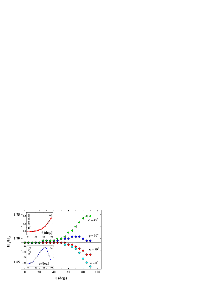
Figure 4: (Color online) The ratio $H_{c3}/H_{c2}$ as a function of polar angle $\theta$ for $\varphi=0$, 30, 45, and 90 degree. Insets: (a) angular dependence of $H_{c2}(\theta)$; (b) $H_{c3}/H_{c2}(\varphi)$ for $\theta=90^{\circ}$.

The sample investigated in the present work is composed of randomly oriented grains with average size of about 40 nm and evenly distributed $H_{c3}$. The observed complete screening of ac field shows that the whole sample surface is in SSS. The onset of the screening could be considered as the percolation transition and the appearance of the large continuous clusters in SSS. Percolation transition in SSS of Nb was discussed in Ref. JUR .

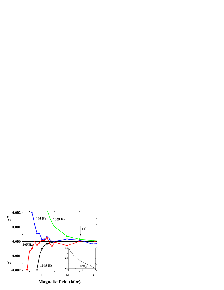
Figure 5: (Color dependence) Magnetic field dependence of $\chi^{\prime}$ and $\chi^{\prime\prime}$ at $T=34$ K in high magnetic fields. $H^{*}$ is shown for $\omega/2\pi=1065$ Hz. The inset shows fraction of grains in SSS, $x$, as a function of $H_{0}/H^{c}_{c3}$.

Fig. 5 shows the expanded view of $\chi^{\prime}$ and $\chi^{\prime\prime}$ at large fields and $T=34$ K at two frequencies $\omega/2\pi=105$ and 1065 Hz. The physical nature of the displacement of the curves along the $H$-axis with frequency is not clear yet, but the response at 1065 Hz gives a more accurate value of the field $H^{*}$, at which the percolation transition takes place. The $H^{*}$ found from $\chi^{\prime}$ equals 11.5 kOe. The $H_{c2}$ at $T=34$ K is about 14.5 kOe. Using the calculated above $\gamma$=2.9, one could find that parallel to the $c$-axis $H_{c3}^{c}$ is about 8.5 kOe and $H^{*}/H_{c3}^{c}\approx 1.35$. Assuming random uniform distribution of $c$-axis orientation in the grains and $H_{c3}(\theta\varphi)/H_{c2}(\theta)\cong 1.7$ we calculated the fraction of the grains in SSS on the surface as a function of dc magnetic field, $x(H_{0})=\int_{0}^{\pi/2}\sin(\theta)\Theta(1.7H_{c2}-H_{0})d\theta$. The result of this calculation is shown in the inset to Fig. 5. The value $H^{*}/H_{c3}^{c}=1.35$ corresponds to the fraction of superconducting grains $x\approx 0.66$. One could infer that $\chi^{\prime\prime}$ provides a more accurate onset for SSS, then $H^{*}=12.5$ kOe and $x\approx 0.58$. These values are in good agreement with the result for critical concentration of conducting clusters $x_{c}=0.6$ in the $2d$ percolation site problem GANT . We consider this as an additional argument in favor of the surface nature of the observed ac response.

The adequateness of the GL model for the description of MgB₂ was discussed recently in  KG in frame of the Usadel equations. In the dirty limit, the GL model is correct if the dimensionless parameter $\eta=q^{2}D_{c}/2\pi T$ is less than 1. Here $q\approx 1/x_{0}$ is the average Fourier component of $f_{s}(x)$ in Eq. (2) and $D_{c}$ is the diffusion coefficient through which the tensor $\widehat{\mu}$ could be expressed GUR . To be sure that calculations of $H_{c2}$ and $H_{c3}$ are correct we found parameter $\eta$ for the most sensitive orientation of $c$-axis, $\overrightarrow{H_{0}}\perp c$ and $\varphi=\pi/2$ assuming that $x_{0}$ is the distance at which the order parameter in the $\pi$-band decreases by the factor of three. It was found that $\eta<1$ for $T/T_{c}>0.8$ and GL equations could be used at $T/T_{c}>0.8$. Another argument in favor of the GL equations is the very good agreement between the temperature dependence of $H_{c3}/H_{c2}$ for $H_{0}$ in $ab$ plane calculated from Eq. (1) and the result obtained in DG on the basis of Usadel model.

In summary, we have demonstrated the existence of SSS in polycrystalline MgB₂. The SSS coexist with weak bulk magnetization. The ac response is linear at low amplitudes of excitation field. The transition to SSS is of $2d$ percolation character. The frequency dispersion for $\omega/2\pi$ in the interval of 5-1065 Hz shows a maximum in $\chi^{\prime\prime}$, and $\chi^{\prime}$ is proportional to $\ln\omega$. The superconducting current in the grain depends on the orientation of the principal axes and is a function of the instant values of magnetic field and both $k$ and $k_{z}$. The relaxation of $k$ and $k_{z}$ to their equilibrium values with zero surface current determines the ac response of the grain. The subsequent averaging over all grains provides a complex character of the observed ac response. We found that GL equations adequately describe the equilibrium dc magnetization of MgB₂ samples at large field and could be used for analysis of SSS. It was shown that the ratio $H_{c3}/H_{c2}$ weakly depends on the orientation of the $c$-axis whereas both $H_{c2}$ and $H_{c3}$ strongly depend on the orientation, which leads to the coexistence of SSS and weak bulk dc magnetic response.

This work was supported by the Klatchky foundation for superconductivity. We wish to thank E.B. Sonin for many helpful discussions.

References

- (1) D. Saint-James and P.G. Gennes, Phys. Lett. 7, 306 (1963).
- (2) R.W. Rollins and J. Silcox, Phys. Rev. 155, 404 (1967).
- (3) L. Lyard et al., Phys. Rev. B 66, 180505(R) (2002).
- (4) A. Rydh et al., Phys. Rev. B 68, 172502 (2003).
- (5) T.C. Shields et al., Supercond. Sci. Technol. 15, 202 (2002).
- (6) D. Shoenberg, Magnetic oscillations in metals, (Cambridge University Press, Cambridge, 1984).
- (7) G.I. Leviev et al., Phys. Rev. B 71, 064506 (2005).
- (8) M.I. Tsindlekht et al., Phys. Rev. B 73, 104507 (2006).
- (9) P.C. Canfield, S.L. Bud’ko and D.K. Finnemore, Physica C 385, 1 (2003).
- (10) A. Gurevich, Phys. Rev. B 67, 184515 (2003).
- (11) I.N. Askerzade, A. Gencer and N. Gülçü, Supercond. Sci.Technol., 15, L13 (2002).
- (12) M.E. Zhitomirsky and V.-H. Dao, Phys. Rev. 69, 054508 (2004).
- (13) V.G. Kogan et al., Phys. Rev. B 65, 094514 (2002).
- (14) V.G. Kogan and J.R. Clem, Phys.Rev. B 24, 2497 (1981).
- (15) V.G. Kogan, S.L. Bud’ko, Physica C, 385 131 (2003).
- (16) A. Rydh et al., Phys. Rev. B 70, 132503 (2004).
- (17) M. Zehetmayer et.al., Phys. Rev. B 66, 052505 (2002).
- (18) U. Welp et al., Phys. Rev. B 67, 012505 (2003).
- (19) J. Kötzler, L. von Sawilski, and S. Casalbuoni, Phys. Rev. Lett. 92, 067005-1 (2004).
- (20) S. Kirkpatrick, Rev. Mod. Phys. 45, 574 (1973).
- (21) A.E. Koshelev and A.A. Golubov, Phys. Rev. Lett., 92, 107008 (2004); A.A. Golubov, A.E. Koshelev, Physica C, 408-410, 338 (2004).
- (22) D.A. Gorokhov, Phys. Rev. Lett., 94, 077004 (2005).