The Finite Size Error in Many-body Simulations with Long-Ranged Interactions

Abstract

We discuss the origin of the finite size error of the energy in many-body simulation of systems of charged particles and we propose a correction based on the random phase approximation at long wave lengths. The correction comes from contributions mainly determined by the organized collective oscillations of the interacting system. Finite size corrections, both on kinetic and potential energy, can be calculated within a single simulation. Results are presented for the electron gas and silicon.

The accurate calculation of properties of systems containing electrons is a very active field of research. Among the possible numerical approaches, quantum Monte Carlo methods are unique in their ability to produce reliable ground state properties at a reasonable computational costFoulkes et al. (2001). However, in the simulation of bulk systems, calculations are necessarily performed using a finite number of electrons with a consequent loss in accuracy. In order to reduce this bias, the system and, hence, the pair interaction are made periodic in a supercell with basis vectors $\{\mathbf{L}_{\alpha}\}_{\alpha=1,2,3}$. (In the case of a crystal these vectors define a supercell of the unit cell.) This is achieved by using the Fourier components of the interaction at the reciprocal wave vectors of the supercell, i.e. $\mathbf{G}$ such that $\exp(i\mathbf{G}\mathbf{L}_{\alpha})=1$. Singular long-ranged potentials, such as the Coulomb interaction, are computed by splitting the sum into a portion in real and reciprocal spaceNatoli and Ceperley (1995). Although using the periodized potential reduces the finite-size effects, some error still remains; the one on the energy, for example, often exceeds the statistical noise and other errors characteristic of quantum simulationsfoo (a). Finite size scaling is possible, but difficult, because the cost of a simulation increases rapidly with the number of particles in the supercell. Here we present an approach that reduces the finite size errors.

In Fourier space and atomic units, the electron-electron potential is:

$$V_{e-e}=\frac{2\pi e^{2}}{\Omega}\sum_{\mathbf{G}\neq 0}\frac{1}{G^{2}}(\rho_{\mathbf{G}}\rho_{-\mathbf{G}}-N)$$ (1)

where $\rho_{\mathbf{G}}\equiv\sum_{i}\exp(i\mathbf{G}\mathbf{r}_{i})$ is the Fourier transform of the charge density, $\Omega$ the volume of the supercell and $N$ the total number of particles. The boundary conditions on the wave function can be chosen as $\Psi(..\mathbf{r}_{i}+\mathbf{L}_{\alpha}..)=\exp(i\theta_{\alpha})\Psi(..\mathbf{r}_{i}..)$ where $\theta_{\alpha}$ is the “twist” of the phase in the $\alpha^{\text{th}}$ direction. Periodic boundary conditions have $\theta_{\alpha}=0$. When there is no long range order, finite size errors are reduced by averaging over twists (i.e. k-point sampling or Brillioun zone integration)Lin et al. (2001). This comes at little cost in simulations since the average is also effective in reducing the statistical noise. Even when this is done, the expectation value of the potential energy remains expressed as a series over $\mathbf{G}$ vectors and is determined by the static structure factor $S_{N}(\mathbf{G})=\langle\rho_{\mathbf{G}}\rho_{\mathbf{-G}}\rangle/N$. As the system size increases, the mesh of $\mathbf{G}$ vectors gets finer and the series eventually converges to an integral corresponding to the exact thermodynamic limit.

The error using a simulation box with $N$ particles is therefore given by

$$\Delta V\equiv\frac{e^{2}}{4\pi^{2}}\int\frac{S_{\infty}(\mathbf{k})-1}{k^{2}}d\mathbf{k}-\frac{2\pi e^{2}}{\Omega}\sum_{\mathbf{G}\neq 0}\frac{S_{N}(\mathbf{G})-1}{G^{2}}.$$ (2)

Its leading order contribution is given by the Madelung constant, $v_{M}$, and corresponds to the difference $-e^{2}\int(2\pi k)^{-2}d\mathbf{k}+2\pi e^{2}\Omega^{-1}\sum_{\mathbf{G}\neq 0}G^{-2}$. It scales as $1/L$ because of the omission of the $G=0$ contribution from the sum and its value is proportional to $e^{2}\int_{\mathcal{D}}(2\pi k)^{-2}d\mathbf{k}$ where $\mathcal{D}$ is a domain of volume $(2\pi)^{3}/\Omega$.

Although $v_{M}$ is generally introduced using a real space picture, as the interaction between images, the above perspective can be easily generalized to the next order correction. The remaining part of the error is determined by i) the substitution of $S_{\infty}(\mathbf{k})$ by the computed $S_{N}(\mathbf{G})$ and ii) the discretization of the integral of $e^{2}S(\mathbf{k})(4\pi^{2}k^{2})^{-1}$. The behavior of $S(\mathbf{k})$ at large $k$ is determined by the short range correlation and can be neglected. This is apparent if the potential is decomposed in a short and long range part. The long range part, whose expectation value is affected by the finite size, decays quickly to $0$ in reciprocal space so that the behavior of $S(\mathbf{k})$ at large $k$ is irrelevant. Moreover, in the limit $k\rightarrow 0$, one knows that the random-phase approximation becomes exact and describes independent density-fluctuation modesNozieres and Pines (1999). In the small $k$ region the random-phase approximation suggests

$$S_{\infty}(\mathbf{G})\simeq S_{N}(\mathbf{G})$$ (3)

and implies that the leading order contribution to the error comes from point ii) above. It is an integration error that, analogously to the Madelung constant, comes from the omission of the $\mathbf{G}=0$ volume element from the energy sum. Scaling of the finite size errors is then determined to leading order by this missing contribution i.e. $e^{2}\int_{\mathcal{D}}S(\mathbf{k})(4\pi k^{2})^{-1}d\mathbf{k}$ where $\mathcal{D}$ is a domain centered on $\mathbf{k}=0$ whose volume equals $(2\pi)^{3}/\Omega$. This, together with the characteristic quadratic behavior of $S(\mathbf{k})$ for correlated charged systems, leads straightforwardly to the well known $1/\Omega$ scaling of the error. foo (b) Thanks to the validity of the random-phase approximation, $S(\mathbf{k})$ can be determined in the small-$k$ region either analytically or from a knowledge of the $S_{N}(\mathbf{k})$ computed in the simulation. Once $S(\mathbf{k})$ is known, one can accurately compute the correction.

We looked at jellium as a test case to judge to what extent Eq.3 is verified. Results for $S_{N}(k)$ computed in variational Monte Carlo simulations at $r_{s}=10$ for 12, 24 and 54 particles are shown in Fig.1.

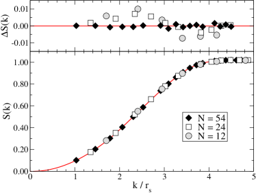
Figure 1: Lower panel: Static structure factor for the electron gas at $r_{s}=10$. Upper panel: $\Delta S=S_{N}(k)-S_{66}(k)$. The difference is computed using a spline function interpolation of $S_{66}$.

As we increase the number of particles, the grid of $k$ points for which $S_{N}$ is defined shifts, but the values of $S_{N}$ fall on a smooth curve, independent of $N$.

Let us now consider the kinetic energy. It is important to distinguish between the effects due to momentum quantization and long range correlation. When using a twisted boundary condition $\bm{\theta}$ in a cubic cell, the kinetic energy is given in terms of the momentum distribution by

$$T=\frac{\hbar^{2}}{2m}\sum_{\mathbf{G}}n_{N}(\mathbf{G}+\bm{\theta}/L)(\mathbf{G}+\bm{\theta}/L)^{2}$$ (4)

When using a single twist, for example periodic boundary conditions, the finite size error is, once again, composed of two contributions: the integration error and the error in approximating the exact momentum distribution, $n_{\infty}$, with $n_{N}$. To better understand the latter point, consider the fourier transform of the momentum distribution: the one-body density matrix. This is equal to the integral over particle coordinates of $\Psi^{\dagger}(\mathbf{r}_{1}+\mathbf{r},\mathbf{r}_{2}...)\Psi(\mathbf{r}_{1},\mathbf{r}_{2}...)$ and converges to the exact one as soon as the correlation length is less than the size of the simulation box. Under the assumptions of no long range correlation, this criterion is eventually met so one has $n_{N}(\mathbf{k})=n_{\infty}(\mathbf{k})$ and the error comes again from approximating the thermodynamic integral with a sum. At variance with the potential energy case, a change in the twist modifies the grid over which the kinetic energy is computed (see Eq.4) so that the error can be made arbitrarily small by increasing the density of twist angles. One can get away with a small number of special $k$-point in the case of semiconductorsRajagopal et al. (1994) but a finer grid is needed for a Fermi liquid due to the discontinuity at the Fermi surface. In the latter case the occupation of the single-particle states varies with the twist and one can use the grand-canonical ensemble to eliminate this source of errorLin et al. (2001).

Consider now the effects due to long range correlation. In Coulomb systems the interaction causes the wave function to have a charge-charge correlation factor: the Jastrow potential. Within the random phase approximation the ground state of the system is described by a collection of dressed particles interacting via short range forces and quantized coherent modes, the plasmons. Accordingly, the many-body wave function factorizes asBohm and Pines (1953)

$$\Psi=\Psi_{\text{s.r.}}\exp\left[-\frac{1}{2\Omega}\sum_{\mathbf{G}\neq 0}u_{\mathbf{G}}\rho_{\mathbf{G}}\rho_{\mathbf{G}}^{\dagger}\right]$$ (5)

where $\Psi_{\text{s.r.}}$ only contains short range correlations and $u_{\mathbf{G}}$ decays quickly to $0$ as $G$ increases and diverges as $G^{-2}$ at small $G$. Because of this divergence, $n_{N}$ converges very slowly to its thermodynamic value and the average over twists provides only a partial correction. Although one can address the bias on the momentum distributionMagro and Ceperley (1994) directly, we here employ a different route. Thanks to Green’s identity the kinetic energy is written as $T=-\left\langle\hbar^{2}\nabla^{2}\ln\psi\right/4m\rangle$McMillan (1965) with a contribution coming from the Jastrow potential given by

$$T_{N}=-\frac{\hbar^{2}}{4m\Omega}\sum_{\mathbf{G}\neq 0}G^{2}u_{\mathbf{G}}\left[S(\mathbf{G})-1\right].$$ (6)

Hence the error of the kinetic energy also has the form of Eq.2: a $1/\Omega$ finite size error in the kinetic energy corresponding to the omission of the $\mathbf{G}=0$ term in Eq.6foo (c). This is an integration error provided $u_{k}$ does not depend on the system size. This must be the case whenever Eq.3 is satisfied since a difference in $u_{k}$ would necessarily imply a difference in $S(\mathbf{k})$.

Errors in the potential and kinetic energy have therefore a very similar mathematical structure. To compute the two corrections we use the Poisson sum formula $\sum_{\mathbf{L}}\widetilde{\zeta}(\mathbf{L})=\Omega^{-1}\sum_{\mathbf{G}}\zeta(\mathbf{G})$ where $\widetilde{\zeta}$ and $\zeta$ are a Fourier transform pair. By separating the $\mathbf{L}=0$ and $\mathbf{G}=0$ contributions from the two sums we get the expression for the error

$$\Delta_{N}\equiv\frac{1}{(2\pi)^{3}}\int\zeta(\mathbf{k})d\mathbf{k}-\sum_{\mathbf{G}\neq 0}\frac{\zeta(\mathbf{G})}{\Omega}=\frac{\zeta(0)}{\Omega}-\sum_{\mathbf{L}\neq 0}\widetilde{\zeta}(\mathbf{L}).$$ (7)

One sets $\zeta(0)$ equal to the $k=0$ limit of $2\pi e^{2}S(k)k^{-2}$ or $\hbar^{2}k^{2}u(k)/4m$ for the correction to the potential and kinetic energy respectively.

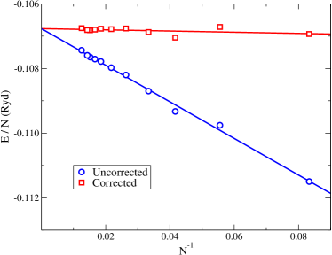
Figure 2: Energies per particle of the electron gas at $r_{s}=10$ in Rydberg as a function of the inverse particle number. Circles are the Monte Carlo energies averaged over twist angles. Squares are the energies after the additional $\hbar\omega_{p}/2N$ correction (see text).

We first apply these corrections to the electron gas for which the small $k$ limits of $S(k)$ and $u(k)$ are known from the random phase approximation as, respectively, $\hbar k^{2}/2m\omega_{p}$ and $4\pi e^{2}/\hbar\omega_{p}k^{2}$ where $\omega_{p}$ is the plasma frequency. In our tests, the wave function had a backflow-Jastrow formHolzmann et al. (2003) and simulations were performed in the grand-canonical ensemble. Thanks to the translational invariance of the Hamiltonian, the wave function factorizes as $\exp(i\bm{\theta}\sum_{i}\mathbf{r}_{i}/L)\Phi$ where $\Phi$, the periodic part, is invariant in a finite pocket of $k$-space around each twist angle. In each pocket the energy dependence on $\bm{\theta}$ is trivial and one can exploit this fact to reduce the number of twist angles to be the number of inequivalent pockets. This, together with cubic symmetry, drastically reduces the number of needed twist angles to between $20-200$ for an unpolarized system with $N\sim 10-100$. The leading order correction due to long range correlations to kinetic and potential energy are equal and sum up a total error $\Delta_{N}=\hbar\omega_{p}(2N)^{-1}$. Corrected and uncorrected variational energies are shown in Fig.2 for $r_{s}=10$. Diffusion Monte Carlo values are uniformly shifted to lower energy by 0.6 mRyd/electron and show similar behavior. One can see that the bias due to the small size of the simulation cell is tremendously reduced, so that the $N=12$ case is already satisfactory.

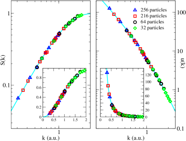
Figure 3: Structure factor (left) and Jastrow potential (right) for diamond silicon at ambient pressure. The continuous lines are fit to the data (see text). The Jastrow potential shows a $k^{-2}$ divergence at small $k$ that was not explicitely imposed but obtained through energy variance minimization using the casino code.

As a second example we considered the diamond structure of silicon at ambient pressure ($r_{s}=2.0$). Calculations were performed using the casinoNeeds et al. (2004) code, a Slater-Jastrow wave function, a Hartree-Fock pseudopotentialTrail and Needs (2005a, b) and periodic boundary conditions. The orbitals used for the trial function (Hartree-Fock) were from the crystal98 codeSaunders et al. (1998). To eliminate the effects of momentum quantization we used a correction based on the density functional eigenvalues of those single-particle states periodic in the simulation cell. Although this is quite common practice it involves another uncontrolled approximation and results depend weakly on the functional employed (we used the local density approximation). The parameters in the Jastrow potential and a one-body term were optimized. The two-particle Jastrow factor was made up by a spherical short range part and a plane wave expansion including 3 shells of k-pointsDrummond et al. (2004). One needs the plane wave expansion to accurately reproduce the behavior of the exact Jastrow factor at small $k$, especially in the case of small simulation cells. To further eliminate errors in the wave function we correct the diffusion Monte Carlo value of $S(k)$ by $S_{\mathbf{G}}^{\text{DMC}}-S_{\mathbf{G}}^{\text{VMC}}$ which leads to an estimate correct to second-order in the wave function.

For Eq.7 we assumed $S(k)=1-\exp(-\alpha k^{2})$ and $u(k)=4\pi a[k^{-2}-(k^{2}+a^{-1})^{-1}]$Becker et al. (1968). When $k$ is expressed in atomic units, the optimal value of $\alpha$ and $a$ were found to be $0.72$ and $1.0$ respectively, leading to corrections of $0.13/N$ and $0.092/N$ hartree per electron for potential and kinetic energy. Results after the two corrections were applied are shown in Fig.4. Even for the smallest cell (cubic, with 8 Si atoms), the error in the energy is of the order of 1 mHartree/electron (0.1 eV/atom) when compared to the value extrapolated for the infinite size.

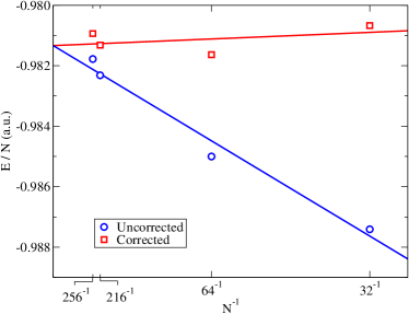
Figure 4: Diffusion Monte Carlo energies per electron in diamond Silicon at $r_{s}=2.0$. Energies and the $S(k)$ and $u(k)$ used to compute the correction are all obtained in simulations with the same number of particles. The smallest cell is the conventional fcc cubic cell of diamond. The two intermidiate ones are, respectively, $2\times 2\times 2$ and $3\times 3\times 3$ supercells of the primitive cell. The largest one is a $2\times 2\times 2$ supercell of the conventional cubic cell.

To conclude, we propose a way to estimate the errors in the potential and kinetic energy under the assumption that the low $k$ behavior of the correlation factor is unchanged upon variation of the simulation cell size. This scheme is suggested by the random-phase approximation that describes independent collective mode in the limit $k\rightarrow 0$. The dominant finite size errors on potential and kinetic energy are integration errors that can be estimated by using the properties of the charge structure factor and the Jastrow potential at long wavelength. The behavior of these quantities in the small $k$ limit can either be obtained analytically (e.g. for the electron gas) or from results with accurate optimized trial wave functions. This approach can be used to obtain energies close to the thermodynamic limit without performing a scaling analysis using different sized systems or assuming the finite-size behavior is given by Fermi liquid theory or approximated by density functional theory.

This material is based upon work supported in part by the U.S Army Research Office under DAAD19-02-1-0176. Computational support was provided by the Materials Computational Center (NSF DMR-03 25939 ITR), the National Center for Supercomputing Applications at the University of Illinois at Urbana-Champaign and by CNRS-IDRIS.

References

- Foulkes et al. (2001) W. M. C. Foulkes, L. Mitas, R. J. Needs, and G. Rajagopal, Rev. Mod. Phys. 73, 33 (2001).
- Natoli and Ceperley (1995) V. Natoli and D. M. Ceperley, J. Comp. Phys. 117, 171 (1995).
- foo (a) For example, the time-step bias and the fixed node error.
- Lin et al. (2001) C. Lin, F. H. Zong, and D. M. Ceperley, Phys. Rev. E 64, 16702 (2001).
- Nozieres and Pines (1999) P. Nozieres and D. Pines, The theory of quantum Liquids (Perseus Books, 1999).
- foo (b) Note, however, that in the Hartree-Fock approximation, metallic systems are characterized by at small so that the error is expected to scale as .
- Rajagopal et al. (1994) G. Rajagopal, R. J. Needs, S. Kenny, W. M. C. Foulkes, and A. James, Phys. Rev. Lett. 73, 1959 (1994).
- Bohm and Pines (1953) D. Bohm and D. Pines, Phys. Rev. 92, 609 (1953).
- Magro and Ceperley (1994) W. R. Magro and D. M. Ceperley, Phys. Rev. Lett. 73, 826 (1994).
- McMillan (1965) W. L. McMillan, Phys. Rev. 138, A442 (1965).
- foo (c) The dominant contribution is given by the “”. The form of the leading order error is .
- Holzmann et al. (2003) M. Holzmann, D. M. Ceperley, C. Pierleoni, and K. Esler, Phys. Rev. E 68, 46707 (2003).
- Needs et al. (2004) R. Needs, M. Towler, N. Drummond, and P. Kent, CASINO version 1.7 User Manual (University of Cambridge, Cambridge, 2004).
- Trail and Needs (2005a) J. R. Trail and R. J. Needs, J. Chem. Phys. 122, 174109 (2005a).
- Trail and Needs (2005b) J. R. Trail and R. J. Needs, J. Chem. Phys. 122, 014112 (2005b).
- Saunders et al. (1998) V. R. Saunders, R. Dovesi, C. Roetti, M. Causa, N. M. Harrison, R. Orlando, and C. M. Zicovich, CRYSTAL98 User’s Manual (University if Torino, 1998).
- Drummond et al. (2004) N. D. Drummond, M. D. Towler, and R. J. Needs, Phys. Rev. B 70, 235119 (2004).
- Becker et al. (1968) M. S. Becker, A. A. Broyles, and T. Dunn, Phys. Rev. 175, 224 (1968).