Theory of Ultracold Superstrings

Abstract

The combination of a vortex line in a one-dimensional optical lattice with fermions bound to the vortex core makes up an ultracold superstring. We give a detailed derivation of the way to make this supersymmetric string in the laboratory. In particular, we discuss the presence of a fermionic bound state in the vortex core and the tuning of the laser beams needed to achieve supersymmetry. Moreover, we discuss experimental consequences of supersymmetry and identify the precise supersymmetry in the problem. Finally, we make the mathematical connection with string theory.

I Introduction

Ultracold quantum gases provide a very exciting branch of physics. Besides the interesting physics that the gases offer by themselves, it has also been possible in the last few years to model with quantum gases systems from other branches of physics, and by doing so to provide answers to long-standing questions. The latter is mainly due to the amazing accuracy by which their properties can be tuned and manipulated. This involves the trapping potential, the dimensionality, the interaction between the atoms, and the statistics. By using a three-dimensional optical lattice the superfluid-Mott insulator transition in the Bose-Hubbard model has been observed Greiner02 . Bosonic atoms confined in one-dimensional tubes by means of a two-dimensional optical lattice where shown to realize the Lieb-Liniger gas Paredes04 ; Kinoshita04 . The unitarity regime of strong interactions was reached by using Feshbach resonances to control the scattering length Regal04 ; Zwierlein04 ; Kinast04 ; Bartenstein04 ; Bournel04 .

To this shortlist of examples from condensed-matter theory, also examples from high-energy physics can be added. In a spinor Bose-Einstein condensate with ferromagnetic interactions skyrmion physics has been studied Khawaja01 ; Ruostekoski01 , whereas an antiferromagnetic spinor Bose-Einstein condensate allows for monopole or hedgehog solutions Stoof01 ; Martikainen02 . There is also a proposal for studying charge fractionalization in one dimension Ruostekoski02 , and for creating (static) non-abelian gauge fields Osterloh05 ; Ruseckas05 . In recent work Snoek05 we have added another proposal to model a system from high-energy physics. By combining a vortex line in a one-dimensional optical lattice with a fermionic gas bound to the vortex core, it is possible to tune the laser parameters such that a nonrelativistic supersymmetric string is created. This we called the ultracold superstring. This proposal combines three topics that have attracted a lot of attention in the area of ultracold atomic gases. These topics are vortices Matthews99 ; Madison00 ; Anderson00 ; Hodby02 ; Fetter01_JP , Bose-Fermi mixtures Hadzibabic02 ; Roati02 ; Inouye04 ; Schori04 ; Goldwin04 ; Stan04 ; Silber05 , and optical lattices Greiner02 ; Stoferle04 . Apart from its potential to experimentally probe certain aspects of superstring theory, this proposal is also very interesting because it brings supersymmetry within experimental reach.

Supersymmetry is a very special symmetry, that relates fermions and bosons with each other. It plays an important role in string theory, where supersymmetry is an essential ingredient to make a consistent theory without the so-called tachyon, i.e., a particle that has a negative mass squared. In the physics of the minimally extended standard model, supersymmetry is used to remove quadratic divergences. This results in a super partner for each of the known particles of the standard model. However, supersymmetry is manifestly broken in our world and none of these superpartners have been observed. A third field where supersymmetry plays a role is in modeling disorder and chaos Efetov . Here supersymmetry is introduced artificially to properly perform the average over disorder. Finally, supersymmetry plays an important role in the field of supersymmetric quantum mechanics, where the formal structure of a supersymmetric theory is applied to derive exact results. In particular this means that a supersymmetry generator $Q$ is defined, such that the hamiltonian can be written as $\mathcal{H}=\{Q,Q^{\dagger}\}$, which is one of the basic relations in the relativistic superalgebra. It is important for our purposes to note, that this relation is no longer enforced by the superalgebra in the nonrelativistic limit. Careful analysis Puzalowski78 ; Clark84 shows that in this limit the hamiltonian is replaced by the number operator, i.e., $\mathcal{N}=\{Q,Q^{\dagger}\}$. It may sometimes be possible to write a nonrelativistic hamiltonian as the anticommutator of the supersymmetry generators, but this does not correspond to the nonrelativistic limit of a relativistic theory.

In our proposal, a physical effect of supersymmetry is that the stability of the superstring against spiraling out of the gas is exceptionally large, because the damping of the center-of-mass motion is reduced by a destructive interference between processes that create two additional bosonic excitations of the superstring and processes that produce an additional particle-hole pair of fermions. Moreover, this system allows for the study of a quantum phase transition that spontaneously breaks supersymmetry as we will show.

Another very interesting aspect of the ultracold superstring is the close relation with string-bit models Bergman95 . These are models that discretize the string in the spatial direction, either to perturbatively solve string theory, or, more radically, to reveal a more fundamental theory that underlies superstring theory. String-bit models describe the transverse degrees of freedom of the string in a very similar fashion as in our theory of the ultracold superstring.

In this article we investigate in detail the physics of ultracold superstrings, expanding on our previous work Snoek05 . The article is organized as follows. In Sec. II we give the detailed derivation of the conditions for the ultracold superstring to be created. In particular, we pay attention to the presence of the fermionic bound state in the vortex core and the tuning of the lasers to reach supersymmetry. In Sec. III we investigate the experimental consequences of the supersymmetry. Sec. IV contains a detailed description of the supersymmetry by studying the superalgebra. In Sec. V we make connection with string theory. Finally, we end with our conclusions in Sec. VI.

II Ultracold superstrings

Our proposal makes use of the fact that a vortex line through a Bose-Einstein condensate in a one-dimensional optical lattice can behave according to the laws of quantum mechanics Martikainen03 . Such an optical lattice consists of two identical counter-propagating laser beams and provides a periodic potential for atoms. When applied along the symmetry axis of a cigar-shaped condensate, which we call the $z$ axis from now on, the optical lattice divides the condensate into weakly-coupled pancake-shaped condensates. In the case of a red-detuned lattice, the gaussian profile of the laser beam provides also the desired trapping in the radial direction. Rotation of the Bose-Einstein condensate along the $z$ axis creates a vortex line that passes through each pancake. Quantum fluctuations of the vortex position are greatly enhanced in this configuration because of the small number of atoms $N_{B}$ in each pancake, which can be as low as $N_{B}=10$, but is typically around $N_{B}=1000$. An added advantage of the stacked-pancake configuration, as opposed to the bulk situation, is that the dispersion of the vortex oscillations is particle like. This ultimately allows for supersymmetry with the fermionic atoms in the mixture. In the one-dimensional optical lattice the vortex line becomes a chain of so-called pancake vortices. This produces a setup which is pictured schematically in Fig 1. There is a critical external rotation frequency $\Omega_{c}$ above which a vortex in the center of the condensate is stable. For $\Omega<\Omega_{c}$ the vortex is unstable, but because of its Euler dynamics, it takes a relatively long time before it spirals out of the gas Anderson00 ; Fedichev99 ; Duine04 . We analyze in detail the case of $\Omega=0$, i.e., the situation in which the condensate is no longer rotated externally after a vortex is created. However, the physics is very similar for all $\Omega<\Omega_{c}$, where supersymmetry is possible. The temperature is taken to be well below the Bose-Einstein condensation temperature, so that thermal fluctuations are strongly suppressed. We only consider the zero-temperature limit, because supersymmetry is formally broken for nonzero temperatures.

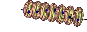
Figure 1: (Color online) Artist’s impression of the setup. The disks represent the bosonic condensate density and the blue balls in the vortex core represent the fermionic density. The black line is a guide to the eye to see the wiggling of the vortex line that corresponds to a Kelvin mode.

II.1 Atomic species

A convenient choice for the boson-fermion mixture is ⁸⁷Rb and ⁴⁰K, since such Bose-Fermi mixtures have recently been realized in the laboratory Roati02 ; Inouye04 ; Schori04 ; Goldwin04 , and because the resonance lines in these two atomic species lie very nearby. The mostly used $|f,m_{f}\rangle$ hyperfine spin states are $|9/2,\pm 9/2\rangle$ and $|9/2,\pm 7/2\rangle$ for ⁴⁰K, and $|2,\pm 2\rangle$, $|1,\pm 1\rangle$, and $|1,0\rangle$ for ⁸⁷Rb Simoni03 . They all have a negative interspecies scattering lenght $a_{BF}$, which is not desirable for our purposes as we show below. It could be possible to use other spin states, which have a positive interspecies scattering length. An other possiblity is to tune the scattering length, using one of the various broad Feshbach resonances that can make the interaction repulsive while keeping the probability to create molecules negligible Simoni03 .

In principle it is also possible to use other mixtures. Another Bose-Fermi mixture that has been realized in the laboratory consists of ²³Na and ⁶Li atoms Hadzibabic02 ; Stan04 . This mixture is less convenient because the resonance lines are widely separated, so that the two species feel very different optical potentials and it is hard to trap both with a single laser. In addition, ⁶Li is relatively hard to trap in an optical lattice because of its small mass. For these reasons, the ²³Na-⁶Li mixture can only be used in a very restricted parameter regime, as we will show lateron in Fig. 5. For the same reasons, the mixture ⁸⁷Rb - ⁶Li Silber05 does not work well either. The mixture ⁷Li-⁶Li Truscott01 ; Schreck01 cannot be used at all, because the resonance lines of the species are the same, so it is impossible to tune the physical properties of the mixture.

II.2 Optical lattice

Because the excited states of the bosonic and fermionic atoms have different transition frequencies, the optical lattice produces for the two species a periodic potential with the same lattice spacing, but with a different height, as schematically shown in Fig. 2.

(a)

(b)

Figure 2: (a) (Color online) Schematic picture of the setup. Here $r$ is the radial distance in the $xy$ plane. The pink and blue blobs represent the bosonic and fermionic densities, respectively. Moreover, $\lambda$ is the wavelength of the laser. The blue and red lines indicate the strength of the optical potential, respectively, for the bosons and fermions as a function of the $z$ coordinate. (b) Schematic fine structure level scheme of the bosonic and fermionic atomic species. Because we consider only sufficiently large detunings the hyperfine level structure is not resolved.

This is very crucial, because it allows to tune the optical lattice for the bosonic and fermionic atoms seperately, by careful adjustement of the wavelength and the Rabi frequency, i.e., the intensity of the laser. This is required to be able to tune the system to become supersymmetric lateron.

For the ⁸⁶Rb-⁴⁰K mixture the Rabi frequencies are in a good approximation the same. For other mixtures the Rabi frequencies are different and we then take the bosonic Rabi frequency as a reference. We take into account the fine-structure level scheme of the atoms, but, assuming that we are sufficiently far from resonance, we neglect the hyperfine structure. As a result, the optical potential is given by

$$V_{B,F}(z)=V_{B,F}\cos^{2}(2\pi z/\lambda),$$ (1)

where the well depths obey

$$V_{B,F} = -\frac{\hbar\Omega_{B,F}^{2}}{3}\left[\left(\frac{1}{\omega^{B,F}_{D_{1}}-\omega}+\frac{1}{\omega^{B,F}_{D_{1}}+\omega}\right)\right.$$

$$\hskip 28.45274pt\left.+2\left(\frac{1}{\omega^{B,F}_{D_{2}}-\omega}+\frac{1}{\omega^{B,F}_{D_{2}}+\omega}\right)\right],$$

$\omega=2\pi c/\lambda$ is the laser frequency, and $\omega_{D_{1}}$ and $\omega_{D_{2}}$ are the frequencies of the $D_{1}$ and $D_{2}$ resonance lines. Here we neglected spontaneous emission of photons. This effect slightly modifies the trapping potential, but gives a finite lifetime to the atoms. Using the rotating-wave approximation and neglecting the fine structure, the effective rate of photon absorption can for red-detuned laser light be estimed as

$$\Gamma_{B,F}^{\rm eff}=-\frac{\hbar\Omega_{B,F}^{2}}{2}\frac{\Gamma_{B,F}}{(\hbar\omega^{B,F}-\hbar\omega)^{2}+(\hbar\Gamma_{B,F})^{2}},$$ (3)

where $\Gamma_{B,F}$ is the linewidth of the bosonic or fermionic excited state, respectively. For blue-detuned laser light, the atoms are trapped in the regions of low laser intensity and spontaneous emission is strongly reduced.

The optical potential should be sufficiently deep to have a bound state for the bosonic and fermionic atoms. To make sure that that is the case we impose the condition

$$\frac{V_{B,F}}{E_{B,F}}>\frac{3}{2},$$ (4)

where we have used the recoil-energy

$$E_{B,F}=\frac{2\pi^{2}}{m_{B,F}\lambda^{2}},$$ (5)

which is the energy associated with the absorption of a photon. On the other hand, the optical lattice should not be so strong to drive the system in the Mott-insulator state Greiner02 ; Stoferle04 ; Oosten03 . In one dimension with many atoms per site, this requires an exceptionally deep lattice, which only occurs if the laser frequency is very close to the resonance frequency of the atomic species. Since we stay away from resonance, this situation does not occur in our calculations.

The wavefunctions in the $z$ direction are assumed to be the groundstate wavefunctions of the harmonic oscillator associated with the optical lattice and thus given by

$$\psi_{B,F}(z)=\frac{1}{\pi^{1/4}\sqrt{\ell_{B,F}^{z}}}\exp\left(-\frac{z^{2}}{2\ell_{B,F}^{z}}\right),$$ (6)

where

$$\ell_{B,F}^{z}=\left(\frac{E_{B,F}}{V_{B,F}}\right)^{1/4}\frac{\lambda}{2\pi}.$$ (7)

For the tunneling amplitude, we use the expression abromowitz

$$J_{B,F}=4\frac{(V_{B,F}^{3}E_{B,F})^{1/4}}{\sqrt{\pi}}\exp\left[-2\sqrt{V_{B,F}/{E_{B,F}}}\right],$$ (8)

which becomes exact for a deep lattice. Therefore, the atomic dispersions along the $z$ axis are given by

$$\epsilon_{B,F}(k)=2J_{B,F}[1-\cos(k\lambda/2)].$$ (9)

Lateron we need for the fermions the relation between the average number of particle per site and the chemical potential $\mu_{F}$. From the above dispersion we derive at zero temperature that

$$N_{F}=\frac{2}{\pi}\arcsin\left[\sqrt{\frac{\mu_{F}}{4J_{f}}}\right],$$ (10)

where we neglect also interaction effects.

II.3 Kelvons

The wavefunction in the (axial) $z$ direction is fully specified by the optical lattice and all the dynamics thus takes place in the radial direction, i.e., in the $xy$-plane. Since the vortex-fluctuations form the lowest-lying modes, we restrict the dynamics to the vortex motion. We follow the derivations in earlier work Martikainen03 ; Martikainen04 , where a specific ansatz for the wavefunction was used, to achieve this. In this work the condensate density was described by a gaussian wavefunction with size $R_{\rm TF}$ and the vortex core was approximated by a step function. Furthermore, it was assumed that the vortex is close to the center. The motion of the vortices results in kelvons, i.e., quantized oscillations of the vortex, described by the creation and annihilation operators

$$\hat{b}=\frac{\sqrt{N_{b}}}{R_{\rm TF}}(\hat{x}+i\hat{y}),\quad\hat{b}^{\dagger}=\frac{\sqrt{N_{b}}}{R_{\rm TF}}(\hat{x}-i\hat{y}),$$ (11)

which obey $[\hat{b},\hat{b}^{\dagger}]=1$. Without the optical lattice Kelvin waves have already been observed Bretin03 ; Mizushima03 . The kelvons have the dispersion

$$\hbar\omega_{K}(k) = \frac{\hbar\omega\ell^{2}}{2R_{\rm TF}^{2}}\left(1-\Gamma\left[0,\left(\frac{l}{R_{\rm TF}}\right)^{4}\right]\right)+\hbar\Omega$$

$$+2J_{K}[1-\cos(k\lambda/2)],$$

where

$$J_{K}=\Gamma[0,(\ell/R_{\rm TF})^{4}]J_{B},$$ (13)

$\Gamma[0,z]$ is the incomplete Gamma function, $R_{\rm TF}$ is the Thomas-Fermi radius in the radial direction, $\ell$ is the bosonic harmonic length in the radial direction, and $\omega$ is the associated frequency. Using another ansatz for the condensate wavefunction can slightly change the constant of proportionality in the definition of the kelvon operators and in the details of the dispersion, but the dispersion always stays tight-binding like.

For the calculation of the bound state in the vortex core, we need to go beyond the description of the core by a step function. This change of the calculation could improve the value of $J_{K}$, but not the functional form of the kelvon dispersion. Since the corrections on the value of $J_{K}$ are small, we just use the result in Eq. (13). Besides the bandwidth $J_{K}$ we derive from Eq. (II.3) also the chemical potential for the kelvons, which gives

$$\mu_{K} \equiv -\hbar\omega_{K}(k=0)$$

$$= \frac{\hbar\omega\ell^{2}}{2R_{\rm TF}^{2}}\left(\Gamma\left[0,\left(\frac{l}{R_{\rm TF}}\right)^{4}\right]-1\right)-\hbar\Omega.$$

Note that the chemical potential is positive only for sufficiently small rotations, which is due to the fact that the vortex is in principle unstable for these values of the rotation and wants to spiral out of the center of the gas cloud.

II.4 Bound states in the vortex core

By treating the interaction between the bosonic and fermionic atoms in mean-field approximation, we have to solve the Gross-Pitaevskii equation for the condensate wavefunction $\Psi({\bf r})$ coupled to the Schrödinger equation for the fermion wavefunction $\psi({\bf r})$

$$(-\frac{\hbar^{2}\nabla_{\bf r}^{2}}{2m_{B}}+\frac{1}{2}m_{B}\omega_{B}^{2}r^{2}-\mu_{B}+\frac{U_{BB}}{2}|\Psi({\bf r})|^{2}+U_{BF}|\psi({\bf r})|^{2}-\hbar\Omega\hat{L}_{z})\Psi({\bf r}) = 0,$$ (15)

$$(-\frac{\hbar^{2}\nabla_{\bf r}^{2}}{2m_{F}}-E+\frac{1}{2}m_{F}\omega_{F}^{2}r^{2}+U_{BF}|\Psi({\bf r})|^{2})\psi({\bf r}) = 0,$$ (16)

which we investigate for the case that $\Omega=0$. The interaction paramaters are related to the scattering lengths according to

$$U_{BB} = \frac{4\pi\hbar^{2}}{\sqrt{2\pi}m_{B}}\frac{a_{BB}}{\ell^{z}_{B}},$$ (17)

$$U_{BF} = \frac{2\pi\hbar^{2}}{\sqrt{\pi}m_{R}}\frac{a_{BF}}{\sqrt{(\ell^{z}_{B})^{2}+(\ell^{z}_{F})^{2}}},$$ (18)

with $a_{BB}$ the boson-boson scattering length and $a_{BF}$ the boson-fermion scattering length and $m_{R}$ the reduced mass $m_{B}m_{F}/(m_{B}+m_{F})$. Although it is very well possible to solve these equations numerically, we prefer an analytic treatment, to gain more insight into the problem. To proceed we make the approximation that the condensate wavefunction is not affected by the presence of the fermions. This is justified, because the contribution of the fermions is ${N_{F}}/{N_{B}}$ smaller than the contribution of the bosons, where $N_{B,F}$ is the average number of bosons and fermions at a lattice site. This ratio will be smaller than $10^{-3}$ as it turns out. Taking into account the interaction with the fermions leads to a slightly wider vortex core, which enhances the possiblity of a bound state. So we first solve the Gross-Pitaevskii equation for the condensate density neglecting the presence of the fermions and then use the condensate density as an effective potential for the fermions. Since we only want to estimate when there is a bound state and we do not need the details of this bound state, we make the following approximations. First, we assume the vortex to be in the center such that the problem is rotationally symmetric and we only have to solve the radial equation. Because of the quantum uncertainty the vortex position in principle fluctuates around the center of the trap, but these fluctuations are small. Second, we assume the envelope condensate wavefunction to be Thomas-Fermi like, i.e.,

$$|\Psi({\bf r})|^{2}=n_{TF}({\bf r})=\frac{\mu_{B}-\frac{m_{B}}{2}\omega_{B}^{2}r^{2}}{U_{BB}}=n_{0}\left(1-\frac{r^{2}}{R_{\rm TF}^{2}}\right).$$ (19)

Third, we describe the vortex core by ${r^{2}}/(r^{2}+2\xi^{2})$ Baym04 , such that the total bosonic density is given by

$$n_{B}({\bf r})=\left(\frac{r^{2}}{r^{2}+2\xi^{2}}\right)n_{TF}({\bf r}).$$ (20)

If we take for the healing length $\xi$ the usual expression in the center of the trap, i.e.,

$$\xi=\frac{\hbar}{\sqrt{2m_{B}n_{TF}(0)U_{BB}}},$$ (21)

we obtain the relation

$$\frac{\xi}{\ell}=\frac{\ell}{R_{\rm TF}}.$$ (22)

By expressing the energy in terms of $\mu_{B}m_{B}/m_{F}$ we can write the Schrödinger equation for the fermions as

$$\left[-\frac{\xi^{2}\nabla_{r}^{2}}{2}-\epsilon+\frac{r^{2}\xi^{2}}{(\ell_{F}^{r})^{4}}+\frac{m_{F}}{m_{B}}\frac{U_{BF}}{U_{BB}}\frac{r^{2}}{2\xi^{2}+r^{2}}\left(1-\frac{r^{2}\xi^{2}}{\ell^{4}}\right)\right]\psi(r)=0,$$ (23)

where $\epsilon=m_{F}E/\mu_{B}m_{B}$ and the dimensionless parameter

$$\Gamma=\frac{m_{F}}{m_{B}}\frac{U_{BF}}{U_{BB}}=\frac{1}{2}\sqrt{\frac{2}{1+\sqrt{\frac{V_{B}}{V_{F}}\frac{E_{F}}{E_{B}}}}}\left(1+\frac{m_{F}}{m_{B}}\right)\frac{a_{BF}}{a_{BB}}$$ (24)

determines whether or not there is a bound state in the core of the vortex.

If we assume that $\xi\ll\ell$ and $\xi\ll\ell_{r}^{F}$, we can neglect the harmonic confinement and the Thomas-Fermi profile of the Bose-Einstein condensate. The effective potential for the fermionic atoms is then given by $\Gamma r^{2}/(r^{2}+2\xi^{2})$. This potential has a bound state for each value of $\Gamma$, because for large distances from the core, it behaves as $\Gamma(1-2\xi^{2}/r^{2})$. However, the size of the wavefunction describing the bound state becomes extremely large for small values of $\Gamma$. Hence it is necessary to take into account the exact form of the potential to make a quantitative estimate of the existence of the bound state. The potential is determined by the values of the radial bosonic and fermionic harmonic length $\ell$ and $\ell_{F}^{r}$. Since $\ell_{F}^{r}$ determines the potential outside the condensate, it determines whether or not the fermions can tunnel out of the core to this region. For the existence of the bound state we can neglect this contribution, which is always justified, because it enhances the possibility of having a bound state.

The radial bosonic harmonic length $\ell$ is fixed by the normalization of the condenstate wavefunction

$$\int d^{2}{\bf r}|\Psi({\bf r})|^{2}=\int d^{2}{\bf r}\frac{r^{2}}{r^{2}+2\xi^{2}}n_{TF}({\bf r})=N_{B}.$$ (25)

Neglecting the presence of the core we find the usual expression for the Thomas-Fermi profile

$$\frac{\ell^{4}}{\xi^{4}}=\frac{R_{\rm TF}^{4}}{\ell^{4}}=\frac{4m_{B}N_{B}U_{BB}}{\pi\hbar^{2}}=\frac{16\sqrt{2\pi}N_{B}a_{BB}}{\lambda}\left[\frac{V_{B}}{E_{B}}\right]^{1/4}\!.$$ (26)

Using that

$$\int d^{2}{\bf r}\left(\frac{r^{2}}{r^{2}+2\xi^{2}}\right)\left(1-\frac{r^{2}}{R_{\rm TF}^{2}}\right)=$$

$$\hskip 2.84544pt\frac{\pi}{2}R_{\rm TF}^{2}+2\pi\xi^{2}\left(1-\left[1+\frac{2\xi^{2}}{R_{\rm TF}^{2}}\right]\log\left(\frac{R_{\rm TF}^{2}+2\xi^{2}}{2\xi^{2}}\right)\right),$$

we see that taking into account the core implies that we have to solve the equation

$$\frac{\ell^{4}}{\xi^{4}}=\frac{4m_{B}N_{B}U_{BB}}{\pi\hbar^{2}}+4\left(1+\frac{2\xi^{4}}{\ell^{4}}\right)\log\left(1+\frac{\ell^{4}}{2\xi^{4}}\right)-4,$$ (27)

where the last two terms come form the presence of the core. Since the core is small in this approximation, this results in a radial harmonic length that is only slightly modified. The requirement that the wavefunction should vanish well within the condensate can then be quantified to yield the expression

$$\Gamma\frac{\sigma^{2}}{\sigma^{2}+2\xi^{2}}\left(1-\frac{\sigma^{2}\xi^{2}}{\ell^{4}}\right)<\epsilon,$$ (28)

where $\sigma$ is the radial size of the fermionic wavefunction. In this way we obtain that for typical densities there is a bound state for $\Gamma>1.5$ which means that ${a_{BB}}/{a_{BF}}>2$.

In contrast to the radial bosonic length $\ell$, the fermionic radial harmonic length $\ell_{F}^{r}$ is not fixed. When the optical lattice is red-detuned, the lattice can be used to trap the atoms also in the radial direction. As a consequence, the total confining potential for the fermions is a multiple of the confining potential of the bosons, i.e.,

$$\frac{r^{2}}{\ell^{2}}+\frac{z^{2}}{(\ell_{B}^{z})^{2}}\propto\frac{r^{2}}{(\ell_{F}^{r})^{2}}+\frac{z^{2}}{(\ell_{F}^{z})^{2}}.$$

This gives the relation

$$\frac{\ell_{F}^{r}}{\ell}=\frac{\ell_{F}^{z}}{\ell_{B}^{z}},$$ (29)

from which we derive

$$\left(\frac{\ell_{F}^{r}}{\xi}\right)^{4}=\left(\frac{\ell_{F}^{z}}{\ell_{B}^{z}}\frac{\ell}{\xi}\right)^{4}=\left(\frac{\ell}{\xi}\right)^{4}\frac{E_{F}}{E_{B}}\frac{V_{B}}{V_{F}}.$$ (30)

However, if the lattice is blue-detuned or if the radial trapping is tuned independently, this relation is not true. The radial trapping can be tuned by introducing a second running laser in the same direction as the optical lattice, as shown in Fig 3.

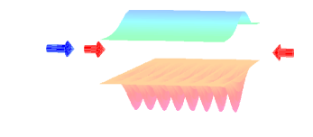
Figure 3: (Color online) Setup with the additional laser to manipulate the radial trapping potential.

The new laser beam has a constant intensity along the $z$ axis, and does not influence the one-dimensional potential wells, but it does change the radial confinement. In principle this second laser also introduces interference terms, but they are much faster than the atoms can follow for the frequencies of interest to us. Therefore, the intensities of the two lasers can simply be added. In particular, as we show lateron, adjusting the radial trapping potentials is needed to get supersymmetric interaction terms. The condition imposed by this requirement is

$$\left(\frac{\ell}{\ell_{F}^{r}}\right)^{4}=\frac{m_{B}}{m_{F}}\left(\frac{\xi}{\ell}\right)^{4}\left(\Gamma\left[0,\left(\frac{\xi}{\ell}\right)^{4}\right]-\frac{3}{2}\right),$$ (31)

which gives the following expression for the fermionic radial harmonic length

$$\left(\frac{\ell_{F}^{r}}{\xi}\right)^{4}=\frac{m_{F}}{m_{B}}\left(\frac{\ell}{\xi}\right)^{8}\frac{1}{\Gamma\left[0,\left(\frac{\xi}{\ell}\right)^{4}\right]-\frac{3}{2}}.$$ (32)

In this last case, the harmonic radial potential for the fermions is very small. In principle this allows the fermionic atoms to tunnel out of the vortex core, to the region where the condensate density vanishes. However, the tunneling is suppressed by increasing the parameter $\Gamma$. A WKB estimate gives that for $\Gamma>5$ the lifetime of the fermions in the core is larger than a second. This means that ${a_{BB}}/{a_{BF}}>8$. Further increasing this ratio increases this lifetime dramatically. Since adjusting the radial trapping potentials is only needed close to the center of the trap, it is also a possibility to use a second laser with a much smaller waist, such that higher-order contributions from the potential prevent the fermions from tunneling out of the core. For various situations, the effective potential for the fermions is shown in Fig 4.

Figure 4: Effective potential for the fermions. Lengths are measured in units of $\xi$ and energies in units of $\mu_{B}m_{B}/m_{F}$. (a) $\Gamma=.5$, $\ell_{F}^{r}\gg\ell$: No bound state, since the potential is too small. (b) $\Gamma=2.6$, $\ell_{F}^{r}\gg\ell$: Bound state in the core, but possibility to tunnel outside. (c) $\Gamma=2.6$, $\ell_{F}^{r}\simeq\ell$: Bound state in the core, no tunneling possible.

II.5 Interactions

In our superstring realization there are also boson-boson and boson-fermion interactions. The kelvons interact repulsively among each other when $\Omega<\Omega_{c}$. For $\Omega=0$ the kelvon-kelvon interaction coefficient is given by Martikainen04B

$$V_{KK}=\frac{\hbar^{2}}{2N_{B}m_{B}R_{\rm TF}^{2}}\left(\Gamma[0,\left({\ell}/{R_{\rm TF}}\right)^{4}]-\frac{3}{2}\right).$$ (33)

In addition, a repulsive interaction between the kelvons and the fermionic atoms is generated by the fact that physically the presence of a kelvon means that the vortex core is shifted off center, together with the fermions trapped in it. Because of the radial confinement experienced by the trapped fermions, this increases the energy of the vortex. When the vortex core is shifted from $0$ to $r$, the fermion hamiltonian is extended by a term

$$\mathcal{H}_{KF}=\frac{m_{F}(\omega_{F}^{r})^{2}}{2}r^{2}c^{\dagger}c,$$ (34)

where $c^{\dagger}c$ is the number operator for the fermions in the core. Defining $C_{B,F}$ as the spring constants associated with the radial confinement of the bosonic and fermionic atoms, respectively, and using the definition of the kelvon operators, this translates into

$$\mathcal{H}_{KF}=\frac{C_{F}R_{\rm TF}^{2}}{2N_{B}}c^{\dagger}c\;b^{\dagger}b.$$ (35)

So the kelvon-fermion interaction coefficient is found to be

$$V_{KF}=\frac{C_{F}R_{\rm TF}^{2}}{2N_{B}}.$$ (36)

II.6 Supersymmetry

To obtain a supersymmetric situation we have three requirements. In the first place the hopping amplitudes have to be the same

$$J_{F}=J_{K}\equiv t.$$ (37)

This can be done by adjusting the laser parameters $\lambda$ and $\Omega_{B}$, as shown in Fig 5. The freedom in choosing the wavelength of the laser can be used to minimize the atom loss. In Fig. 6, we plot the atom loss as a function of the wavelength of the laser.

Figure 5: Tuning of the lattice laser to obtain supersymmetry. Plotted is the Rabi frequency for the bosonic atoms versus wavelength for ⁸⁷Rb-⁴⁰K for 10000 (solid line), 1000 (dashed line) and 500 (dotted line) bosonic atoms per site. Note that for the blue-detuned part, i.e., $\lambda<760$ nm for the ⁸⁷Rb-⁴⁰K mixture extra radial trapping is needed, either magnetically, or by using an extra running laser as discussed in the text and shown in Fig. 3. In Fig. 8 we display how to tune the running laser to obtain also supersymmetric interactions. In the inset we plotted the Rabi frequency that is required for the ²³Na-⁶Li mixture to obtain supersymmetry, again for 10000 (solid line), 1000 (dashed line) and 500 (dotted line) bosonic atoms per site. Note that this can only be obtained in a very limited range of wavelength’s.

Figure 6: Effective rate of photon absorption as a function of the wavelength of the optical lattice for 1000 bosonic atoms per site. The solid line is for the bosonic atoms, whereas the dashed line is for the fermionic atoms in the ⁸⁷Rb-⁴⁰K mixture.

Secondly, the chemical potentials have to be the same

$$\mu_{F}=\mu_{K}\equiv\mu.$$ (38)

This can be achieved by adjusting the fermion filling fraction $N_{F}$, as shown in Fig 7. Using the result from Eq. (10) and using the requirements for supersymmetry we obtain

$$N_{F}=\frac{2}{\pi}\arcsin\left(\sqrt{\frac{\frac{\hbar\omega\ell^{2}}{2R_{\rm TF}^{2}}\left(\Gamma\left[0,\frac{l^{4}}{R_{\rm TF}^{4}}\right]-1\right)}{4J_{B}\Gamma\left[0,\frac{l^{4}}{R_{\rm TF}^{4}}\right]}}\right)$$

$$=\!\frac{2}{\pi}\arcsin\!\left(\!\frac{\ell}{\ell_{B}^{z}}\sqrt{\frac{\sqrt{\pi}\frac{\ell^{2}}{R_{\rm TF}^{2}}\left(\Gamma\left[0,\frac{l^{4}}{R_{\rm TF}^{4}}\right]\!-\!1\!\right)e^{\sqrt{\tfrac{V_{B}}{E_{B}}}}}{16(V_{B}/E_{B})^{1/4}\Gamma\left[0,\frac{l^{4}}{R_{\rm TF}^{4}}\right]}}\right)\!.$$

The ratio $\ell/\ell_{B}^{z}$ is undetermined by supersymmetry constraints. In order for the Thomas-Fermi approximation to apply in the radial direction, versus the gaussian wavefunction in $z$ direction, this ratio needs to be sufficiently small. In the figure a ratio of $1/5$ is chosen.

Figure 7: Tuning of the average number of fermions per lattice site to obtain supersymmetry for 10000 (solid line), 1000 (dashed line) and 500 (dotted line) bosonic atoms per lattice site. The result depends on the ratio of the bosonic harmonic lengths in the axial and radial directions $\ell/\ell_{B}^{z}$. This ratio should be sufficiently small to be radially in the Thomas-Fermi limit. For this plot a ratio of 1/5 is chosen.

Finally, the interaction terms have to be the same. This implies

$$V_{KK}=V_{KF}\equiv U.$$ (39)

Setting these coefficients equal to each other gives a condition on the radial trapping given by

$$\frac{C_{F}}{C_{B}}=\left(\frac{\ell}{R_{\rm TF}}\right)^{4}\left(\Gamma[0,\left({\ell}/{R_{\rm TF}}\right)^{4}]-\frac{3}{2}\right).$$ (40)

The radial trapping can be tuned by introducing a second running laser, as explained before. For the second laser, we can again independently choose both the wavelength and the Rabi frequency as shown in Fig. 8. This can again be used to minimize the atom loss due to the red-detuned laser, but it turns out that atom loss is always quite small anyway for reasonable system parameters. Only for very small detunings, the lifetime is less than a second.

Figure 8: Tuning of the additional laser to obtain supersymmetric interactions for 1000 bosonic atoms per lattice site. The Rabi frequency is plotted versus the wavelength of the running laser for different wavelengths of the lattice laser beam: 1000 nm for the left curve and 600 nm for the right curve. In the inset the effective rate of photon absorption originating from the additional laser is plotted, again the left curves are for a lattice laser of 1000 nm and the right curves are for a lattice laser of 1000 nm. The solid lines indicate the rate of photon absorption for the bosonic atoms, whereas the dashed lines are the rates of photon absorption for the fermionic atoms.

II.7 Hamiltonian

Combining everything, our superstring is described by the supersymmetric hamiltonian

$$\mathcal{H} = -t\sum_{\langle ij\rangle}[b_{i}^{\dagger}b_{j}+c_{i}^{\dagger}c_{j}]$$

$$+\sum_{i}\Bigl{[}-\mu^{\prime}(b_{i}^{\dagger}b_{i}+c_{i}^{\dagger}c_{i})+\frac{U}{2}b_{i}^{\dagger}b_{i}^{\dagger}b_{i}b_{i}+Ub_{i}^{\dagger}b_{i}c_{i}^{\dagger}c_{i}\Bigr{]}.$$

Here $b_{i}$ is the annihilation operator of a kelvon at site $i$, $c_{i}$ is the annihilation operator of a fermion at site $i$, $\langle ij\rangle$ means that the summation runs over neighbouring sites, and $\mu^{\prime}=\mu-2t$. We used the convention for the Fourier transformation $f_{k}=(1/\sqrt{N_{s}})\sum_{n}e^{ikz_{n}}f_{n}$, where $N_{s}$ is the number of lattice sites. We define $a=\lambda/2$ as the lattice spacing and $L=N_{s}a$ as the length of the system. Assuming that $N_{s}\gg 1$, such that $L\gg a$, we can perform a continuum approximation to obtain for the hamiltonian

$$\mathcal{H} = \int dz\;b^{\dagger}(z)\left(-\frac{\hbar^{2}}{2m^{*}}\frac{\partial^{2}}{\partial z^{2}}-\mu\right)b(z)$$

$$+\int dz\;c^{\dagger}(z)\left(-\frac{\hbar^{2}}{2m^{*}}\frac{\partial^{2}}{\partial z^{2}}-\mu\right)c(z)$$

$$+\frac{U}{2}\int dz\;[b^{\dagger}(z)b^{\dagger}(z)b(z)b(z)+2b^{\dagger}(z)b(z)c^{\dagger}(z)c(z)],$$

where we introduced the effective mass $m^{*}=\hbar^{2}/2a^{2}t$. This continuum hamiltonian turns out to be exactly solvable Batchelor05 ; Imambekov06 by a straightforward generalization of the Bethe-Ansatz solution of the one-dimensional Bose gas Lieb63 ; Yang67 . However, the exact solutions spontaneously break supersymmetry and do not give much insight in the role of supersymmetry in the problem.

Using that the lagrangian is given by

$$\mathcal{L}=\sum_{i}\left(b_{i}^{\dagger}i\hbar\frac{\partial}{\partial t}b_{i}+c_{i}^{\dagger}i\hbar\frac{\partial}{\partial t}c_{i}\right)-\mathcal{H}[b^{\dagger},b;c^{\dagger},c],$$ (43)

the action in the continuum limit is obtained as

$$S\!\! = \!\!\int\!\!dt\!\int\!\!dz\left\{b^{*}\!\left(\!i\hbar\frac{\partial}{\partial t}+\frac{\hbar^{2}}{2m^{*}}\frac{\partial^{2}}{\partial z^{2}}+\mu\!\right)\!b\right.$$

$$\hskip 31.2982pt+c^{*}\left(\!i\hbar\frac{\partial}{\partial t}+\frac{\hbar^{2}}{2m^{*}}\frac{\partial^{2}}{\partial z^{2}}+\mu\!\right)\!c$$

$$\hskip 42.67912pt-\left.\frac{U}{2}\left(|b|^{2}+|c|^{2}\right)^{2}\right\},$$

which now explicitly shows the supersymmetry of the problem, because it remains invariant when $b$ and $c$ are rotated into each other. If we neglect the interaction terms, which are rather small anyway, the fermions fill a Fermi sea and the low-energy excitations are particle-hole excitations around the Fermi surface. Therefore, the low-energy part of the theory is properly described by linearizing the fermionic dispersion around the Fermi level. To preserve supersymmetry we do the same for the bosons and obtain at the quadratic level the action

$$S\!\! = \!\!\sum_{\sigma=\pm}\!\int\!dt\!\!\int\!dk\Bigl{\{}b_{\sigma}^{*}(k,t)(i\hbar\partial_{t}-\hbar v_{F}(\sigma k-k_{F}))b_{\sigma}(k,t)$$

$$\hskip 48.36958pt+c_{\sigma}^{*}(k,t)(i\hbar\partial_{t}-\hbar v_{F}(\sigma k-k_{F}))c_{\sigma}(k,t)\Bigr{\}},$$

where $\sigma$ indicates whether the particles are right movers or left movers and $v_{F}=\hbar k_{F}/m^{*}$ is the Fermi velocity. We used that $\mu=\hbar^{2}k_{F}^{2}/2m^{*}$. We identify the Fermi velocity with the velocity of light $c$ and perform the transformation $c_{\sigma}(z,t)=(1/\sqrt{L})\sum_{k}e^{ikz}c_{\sigma}(k+\sigma k_{F},t)$. We introduce the Dirac spinor $\psi(z,t)=(c_{+}(z,t),c_{-}(z,t))$ and $\bar{\psi}(z,t)=\psi^{\dagger}(z,t)\gamma^{0}$, with $\gamma^{0}=\sigma_{y}$. The other Dirac matrices are $\gamma^{1}=i\sigma_{x}$ and $\gamma^{5}=\sigma_{z}$. The two bosonic fields can be captured in a single Klein-Gordon field $X(z,t)=(1/\sqrt{L})\sum_{k}e^{ikz}\sqrt{\hbar/k}\left(b_{+}(k+k_{F},t)+b_{-}(k-k_{F},t)\right)$, such that $\partial^{\mu}\partial_{\mu}X=(\partial_{t}^{2}/c^{2}-\partial_{z}^{2})X=0$. This enables us to rewrite the linearized action as

$$S=\int d^{2}x\Bigl{\{}\partial^{\mu}X^{*}\partial_{\mu}X+i\hbar\bar{\psi}\gamma^{\mu}\partial_{\mu}\psi\Bigr{\}},$$ (45)

which is the action for the transverse modes of a free relativistic $N=1$ superstring in $3+1$ dimensions GSW . In modern language, the Lorentz invariance of this action appears here as an emergent phenomenon at long wavelenghts, because the underlying theory is not Lorentz invariant. This is very similar with the way in which Lorentz invariance appears in string-bit models Bergman95 . A second property of this action is, that the fermionic part has classically chiral symmetry, but quantum-mechaniclly suffers from a chiral anomaly. Whereas in string theory this is an unwanted feature, in our case it has a physical origin, because it comes about from the fact that the underlying microscopic theory does not conserve the chiral current $i\bar{\psi}\gamma^{\mu}\gamma^{5}\psi$, and only conserves the current $\bar{\psi}\gamma^{\mu}\psi$ associated with the conservation of the total number of fermions.

II.8 Nonlocal interaction

The presence of a kelvon implies that neighbouring vortex cores are slightly shifted with respect to each other. This effect decreases the fermionic hopping amplitude and results in a interaction term that couples fermions on neighbouring sites of the form

$$\mathcal{H}^{\prime}=t\sum_{kk^{\prime}}A(k^{\prime})\cos(k)c_{k}^{\dagger}c_{k}b_{k^{\prime}}^{\dagger}b_{k^{\prime}}.$$ (46)

Since this term breaks supersymmetry, we want to investigate the system parameters for which it can be neglected, i.e., for which $A(k^{\prime})\ll 1$. To do so we consider a kelvon with a certain wavenumber $k$. The relative distance between neighboring cores kan then be estimated to be

$$\delta r=\frac{R_{\rm TF}}{\sqrt{N_{B}}}\frac{k\lambda}{2}.$$ (47)

From Eq. (20) we know that for small distances the vortex core can be modeled as a harmonic potential with width $\xi$. Hence, the fermionic wavefunctions are gaussians with the same width. So we have to compute

$$A(k) = 1-\frac{\int d^{2}{\bf r}e^{-\frac{{\bf r}^{2}}{2\xi^{2}}}e^{-\frac{({\bf r}-\delta r_{0})^{2}}{2\xi^{2}}}}{\int d^{2}{\bf r}e^{-\frac{{\bf r}^{2}}{\xi^{2}}}}$$

$$= 1-e^{-\frac{\delta r_{0}^{2}}{4\xi^{2}}}\simeq\frac{\delta r_{0}^{2}}{4\xi^{2}}=\frac{k^{2}\lambda^{2}R_{\rm TF}^{4}}{16N_{b}\ell^{4}},$$

where we used the relation from Eq. (26). From this same relation we see that $(R_{\rm TF}/\ell)^{4}$ scales with the number of bosonic atoms $N_{B}$, such that $A(k)$ is independent of $N_{B}$. We can estimate $R_{\rm TF}^{4}/N_{B}\ell^{4}$ to be of order unity, such that the requirement for $A(k)$ to be small only depends on the wavenumber $k$. If we identify this wavenumber with the Fermi momentum, i.e.,

$$\frac{k_{F}^{2}\lambda^{2}}{16}\ll 1,$$ (49)

we obtain a restriction on the fermionic filling fraction which can be estimated to be

$$N_{F}<0.1.$$ (50)

From Fig. 7 we see that for most of the parameter space this condition is fullfilled.

III Experimental signal

It is an important question how the supersymmetry can be observed. Therefore we need to distinguish between the question whether the hamiltonian is tuned to be supersymmetric and whether the quantum ground state is supersymmetric, since it is possible that the ground state can spontaneously break supersymmetry. We are primarely interested in the situation that both the hamiltonian and the quantum ground state are supersymmetric.

III.1 Density measurements

The two observables that are most easy to measure experimentally are the average number of fermions at a site $N_{F}$ and the average number of kelvons $N_{K}$. The average fermion number can be determined by usual absorpsion measurements. The number of kelvons can be obtained from the mean-square displacement $\langle r^{2}\rangle=(1/N_{s})\sum_{i}\langle x_{i}^{2}+y_{i}^{2}\rangle$ of the pancake vortices, which can be measured by imaging along the $z$ direction the size of the circle within which the vortex positions are concentrated Martikainen04 . Because

$$b_{i}^{\dagger}b_{i}=N_{B}\frac{x_{i}^{2}+y_{i}^{2}}{R_{\rm TF}^{2}}-\frac{1}{2},$$ (51)

this can directly be translated to the number of kelvons at a site. It is clear that in order to have a supersymmetric state, the kelvon and fermion modes should have the same average occupation number, i.e.,

$$\langle b_{i}^{\dagger}b_{i}\rangle=\langle c_{i}^{\dagger}c_{i}\rangle.$$ (52)

This allows us to devise an experimental measure for the proximity to the supersymmetric point, which can be directly measured, namely

$$\left(N_{B}\frac{\langle r^{2}\rangle}{R_{\rm TF}^{2}}-N_{F}-{1}/{2}\right)^{2}.$$

This quantity has an absolute minimum of zero at the supersymmetric point, so that it’s magnitude is a measure of the deviation from supersymmetry. We can extend this to higher order correlation functions. The condition that

$$\langle(b_{i}^{\dagger}b_{i})^{2}\rangle=\langle(c_{i}^{\dagger}c_{i})^{2}\rangle=\langle c_{i}^{\dagger}c_{i}\rangle,$$ (53)

can be used to prove that in order to have supersymmetry also the condition

$$N_{B}^{2}\frac{\langle r^{4}\rangle}{R_{\rm TF}^{4}}=2N_{F}+\frac{1}{4}$$ (54)

should hold. The quantiy $\langle r^{4}\rangle$ can again be measured from the distribution of the measured vortex postions.

Figure 9: Diagrams that contribute to the dissipation of the vortex line. The solid lines represent bosonic propagators, the dashed lines represent fermionic propagators. The left diagram is called $\Pi_{KK}(k,\omega)$, the left diagram is called $\Pi_{KF}(k,\omega)$

.

III.2 Dissipation

Another consequence of supersymmetry that can be directly measured is the reduced dissipation. Dissipation in this context results in the vortex spiraling out of the gas. Fedichev99 ; Duine04 . The dominant part of the dissipation is given by the coupling to the kelvon modes and the fermionic modes. The lowest order diagrams are given in Fig. 9 and denoted by $\Pi_{KK}(k,\omega)$ for the coupling to the kelvon modes and $\Pi_{KF}(k,\omega)$ when there is also coupling to the fermionic modes. The imaginary part of these diagrams measures the dissipation. In order to be able to know the dissipation away from the supersymmetric point we perform the calculation for unequal dispersions $\epsilon_{K,F}(k)$ and unequal coupling constant $U_{KK}$ and $U_{KF}$. We introduce the usual notation for the Bose-Einstein and Fermi-Dirac distribution functions

$$N_{B}[\epsilon(k)]=\frac{1}{e^{\epsilon(k)/k_{B}T}-1},\quad N_{F}[\epsilon(k)]=\frac{1}{e^{\epsilon(k)/k_{B}T}+1}.$$

The diagrams are then given by

$$\Pi_{KK}(k,i\omega) = 2U_{KK}^{2}\int\frac{dp}{2\pi}\int\frac{dp^{\prime}}{2\pi}\frac{\Bigl{(}1+N_{B}[\epsilon_{K}(p)]+N_{B}[\epsilon_{K}(p^{\prime})]\Bigr{)}N_{B}[\epsilon_{K}(p+p^{\prime}-k)]-N_{B}[\epsilon_{K}(p)]N_{B}[\epsilon_{K}(p^{\prime})]}{i\hbar\omega-\epsilon_{K}(p)-\epsilon_{K}(p^{\prime})+\epsilon_{K}(p+p^{\prime}-k)}$$

$$\Pi_{KF}(k,i\omega) = -U_{KF}^{2}\int\frac{dp}{2\pi}\int\frac{dp^{\prime}}{2\pi}\frac{\Bigl{(}-1-N_{B}[\epsilon_{K}(p)]+N_{F}[\epsilon_{F}(p^{\prime})]\Bigr{)}N_{F}[\epsilon_{F}(p+p^{\prime}-k)]+N_{B}[\epsilon_{K}(p)]N_{F}[\epsilon_{F}(p^{\prime})]}{i\hbar\omega-\epsilon_{K}(p)-\epsilon_{F}(p^{\prime})+\epsilon_{F}(p+p^{\prime}-k)},$$

where the minus sign in front of the expression for $\Pi_{KF}(k,i\omega)$ comes from the presence of the fermion loop. Note that due to the different combinatorial factors the diagram $\Pi_{BB}$ comes with an extra factor of two, which is lacking in the case of the diagram $\Pi_{BF}$. As a result, the two diagrams do not cancel exactly at the supersymmetric point, as we claimed previously Snoek05 . Instead, the dissipation is reduces by a factor 2 Bernard . The imaginary part of the diagrams gives the following expressions

$${\rm Im}[\Pi_{KK}(k,\omega)] = 2U_{KK}^{2}\int\frac{dp}{2\pi}\int\frac{dp^{\prime}}{2\pi}\Bigl{\{}\delta(\hbar\omega-\epsilon_{K}(p)-\epsilon_{K}(p^{\prime})+\epsilon_{K}(p+p^{\prime}-k))\times$$

$$\hskip 28.45274pt\left(\Bigl{(}1+N_{B}[\epsilon_{K}(p)]+N_{B}[\epsilon_{K}(p^{\prime})]\Bigr{)}N_{B}[\epsilon_{K}(p+p^{\prime}-k)]-N_{B}[\epsilon_{K}(p)]N_{B}[\epsilon_{K}(p^{\prime})]\right)\Bigr{\}},$$

$${\rm Im}[\Pi_{KF}(k,\omega)] = -U_{KF}^{2}\int\frac{dp}{2\pi}\int\frac{dp^{\prime}}{2\pi}\Bigl{\{}\delta(\hbar\omega-\epsilon_{K}(p)-\epsilon_{F}(p^{\prime})+\epsilon_{F}(p+p^{\prime}-k))\times$$ (55)

$$\hskip 28.45274pt\left(\Bigl{(}-1-N_{B}[\epsilon_{K}(p)]+N_{F}[\epsilon_{F}(p^{\prime})]\Bigr{)}N_{F}[\epsilon_{F}(p+p^{\prime}-k)]+N_{B}[\epsilon_{K}(p)]N_{F}[\epsilon_{F}(p^{\prime})]\right).$$

At zero temperature we have that $N_{F}[\epsilon(k)]=\theta(\epsilon(k))$, and $N_{B}[\epsilon(k)]=-\theta(\epsilon(k))=-N_{F}[\epsilon(k)]$. Using this, we see that if there is supersymmetry, i.e., if $\epsilon_{K}(k)=\epsilon_{F}(k)$ and $U_{KK}=U_{KF}$, we have that

$$\Pi_{KK}(k,\omega)=-2\Pi_{KF}(k,\omega),$$

and in particular that

$${\rm Im}[\Pi_{KK}(k,\omega)+\Pi_{KF}(k,\omega)]=\frac{1}{2}{\rm Im}[\Pi_{KK}(k,\omega)],$$

such that at zero temperature supersymmetry results in a dissipation rate that is only half as large as in the case of a ordinary vortex-line. Using these expressions, it is also possible to calculate the quantum dissipation at nonzero temperature, or when supersymmetry is broken. In particular, when the interaction coefficients are tuned away from the supersymmetric point such that $U_{BF}=\sqrt{2}U_{BB}$ and supersymmetry is maintained at the quadratic level, the dissipation exactly vanishes and the superstring is extremely stable in the center of the condensate.

III.3 Spontaneous supersymmetry breaking

When the hamiltonian is supersymmetric, the ground state still can break supersymmetry. This is the phenomenon of spontaneous supersymmetry breaking. For $\Omega<\Omega_{c}$, the ultracold superstring is unstable against Bose-Einstein condensation of kelvons. This breaks supersymmetry, because the fermionic modes cannot Bose-Einstein condense. Bose-Einstein condensation implies that the kelvon annihilation operator obtains an expectation value

$$\langle b_{i}\rangle\neq 0.$$ (56)

From the definition of the kelvon operator we conclude that as a consequence

$$\langle x\rangle^{2}+\langle y\rangle^{2}>0.$$ (57)

This means that the vortex moves out of the center of the trap. Experimentally this is easy to measure. Moreover, by monitoring the vortex position when it moves out of the center of the trap, this also allows for the experimental investigation of the dynamics of supersymmetry breaking. As a consequence of the breaking of the $U(1)$ symmetry because of the Bose-Einstein condensation, the dispersion of the kelvon modes becomes gapless. The dispersion becomes the usual Bogoliubov dispersion, which reads

$$\hbar\omega_{B}(k)=\sqrt{\epsilon(k)^{2}+2\mu\epsilon(k)},$$ (58)

with $\epsilon(k)=\hbar^{2}k^{2}/2m^{*}$. For long wavelengths this yields a linear behaviour. Also the fermionic modes become gapless. This is a result of the breaking of supersymmetry and this mode is called the goldstino. Because $\langle b\rangle=\sqrt{\mu/U}$, the dispersion for the goldstino is given by

$$\hbar\omega_{F}(k)=\epsilon(k)-\mu+|\langle b\rangle|^{2}=\epsilon(k),$$ (59)

which results in a quadratic dispersion. Clearly the bosonic and fermionic dispersion in Eqs. (58) and (59) are now different, which signals a nonsupersymmetric situation.

IV Supersymmetry

In this section we review the algebra associated with supersymmetric field theories both in the relativistic (super Poincaré algebra) and the non-relativistic limit (super Galilei algebra). We give an explicit representation of the super Galilei algebra in terms of the bosonic and fermionic operators.

IV.1 Super Poincaré algebra

Associated with a relatistic field theory in $D=d+1$ dimensions is the Poincaré algebra, whose generators consist of a vector $P^{\mu}$, that generates translations and an antisymmetric tensor $J^{\mu\nu}$, that generates Lorenz transormations. The greek indices run from $0$ to $d=D-1$, such that $P^{0}$ should be identified with the hamiltonian $\mathcal{H}$, up to a constant. The algebra is then given by

$$[P^{\mu},P^{\nu}] = 0$$ (60)

$$[J^{\mu\nu},P^{\rho}] = i(\eta^{\mu\rho}P^{\nu}-\eta^{\nu\rho}P^{\mu})$$

$$[J^{\mu\nu},J^{\rho\sigma}] = i(\eta^{\mu\rho}J^{\nu\sigma}+\eta^{\mu\sigma}J^{\rho\nu}-\eta^{\nu\rho}J^{\mu\sigma}-\eta^{\nu\sigma}J^{\rho\mu}),$$

where $\eta^{\mu\nu}$ is the flat space Minkowski metric. When there is supersymmetry we can extend this to the super Poincaré algebra. For $N=1$ supersymmetry in $1+1$ dimensions this involves the two-component Majorana spinor $Q_{\alpha}$, $\alpha=1,2$, which is the generator of supersymmetry transformations. The algebra is then extended to include also

$$[P^{\mu},Q_{\alpha}] = 0$$ (61)

$$[P^{\mu},\bar{Q}_{\alpha}] = 0$$ (62)

$$[J^{\mu\nu},Q_{\alpha}] = -\frac{i}{4}[\gamma^{\mu},\gamma^{\nu}]_{\alpha\beta}Q_{\beta}$$ (63)

$$\{Q_{\alpha},\bar{Q}_{\beta}\} = 2\gamma_{\alpha\beta}^{\mu}P_{\mu},$$ (64)

where the $\gamma^{\mu}$ are again the Dirac matrices. We use conventions such that $Q_{\alpha}$ has two real components. To make connection with the supersymmetry in the ultracold superstring we combine these two components in one complex supersymmetry operator

$$Q=\frac{Q_{1}+iQ_{2}}{2}.$$ (65)

This decomposition breaks manifest Lorentz symmetry, but since we are ultimately interested in the nonrelativistic limit, this is of no concern to us here. As a result we obtain the following algebra

$$[P^{\mu},Q] = 0$$ (66)

$$[J^{\mu\nu},Q] = -\frac{i}{2}\epsilon^{\mu\nu}Q^{\dagger}$$ (67)

$$\{Q,Q^{\dagger}\} = P^{0}$$ (68)

$$\{Q,Q\} = \{Q^{\dagger},Q^{\dagger}\}=-P^{1}.$$ (69)

In particular, we see that the hamiltonian $P^{0}$ is fixed by the supersymmetry generator. This is a very peculiar restriction on the hamiltonian, which is only true for the relativistic theory. In the nonrelativistic limit, the supersymmetry decouples from the space-time translation symmetry as we show now.

IV.2 Super Galilei algebra

The Galilei algebra can be derived as a limit of the Poincaré algebra by performing a Inönü-Wigner contraction Inonu53 in the following way Puzalowski78 ; Clark84 . We write

$$P^{0} = \frac{1}{c}(m^{*}\mathcal{N}c^{2}+\mathcal{H})$$ (70)

$$P^{1} = P$$ (71)

$$J^{01} = cK$$ (72)

$$Q = \sqrt{c}Q,$$ (73)

where $c$ is the speed of light and $m^{*}$ denotes the mass, which is the same for the bosonic and fermionic degrees of freedom. We also defined a number operator $\mathcal{N}$, which counts all the particles in the system, and boost operators $K$. Furthermore, we still have the space translation generators $P$ and the hamiltonian $\mathcal{H}$. We can now take the limit $c\rightarrow\infty$ to obtain the super Galilei algebra. The Galilei algebra obtained in this manner has nonvanishing commutators

$$[P,K] = im^{*}\mathcal{N}$$ (74)

$$[\mathcal{H},K] = iP.$$ (75)

The part involving the supersymmetry becomes only

$$\{Q,Q^{\dagger}\}=\mathcal{N}.$$ (76)

This defines the algebra $\mathcal{S}_{1}\mathcal{G}$ Bergman95 . As is clear, in this case the hamiltonian is decoupled form the supersymmetry. In $1+1$ and $2+1$ dimensions, it is sometimes possible to define an extended superalgebra $\mathcal{S}_{2}\mathcal{G}$, which again involves the hamiltonian Bergman95 ; Bergman95B ; Bergman96 . In $d=1$ this amounts to introducing an extra scalar supersymmetry generator $R$ with the algebra:

$$\{Q,R^{\dagger}\} = -P$$ (77)

$$\{R,R^{\dagger}\} = \mathcal{H}/2.$$ (78)

IV.3 Representation

The representation for the $\mathcal{S}_{1}\mathcal{G}$ algebra in terms of the bosonic and fermionic operators $b$ and $c$, can easily be found to be

$$\mathcal{N} = \int dz\{b^{\dagger}(z)b(z)+c^{\dagger}(z)c(z)\},$$ (79)

$$P = -\frac{i\hbar}{m^{*}}\int dz\{b^{\dagger}(z)\partial_{z}b(z)+c^{\dagger}(z)\partial_{z}c(z)\},$$ (80)

$$Q = \int dz\;c^{\dagger}(z)b(z),$$ (81)

$$Q^{\dagger} = \int dz\;b^{\dagger}(z)c(z).$$ (82)

In addition, we can thus also define

$$R = \frac{\hbar}{\sqrt{m^{*}}}\int dz\;c^{\dagger}(z)\partial_{z}b(z),$$ (84)

$$R^{\dagger} = -\frac{\hbar}{\sqrt{m^{*}}}\int dz\;b^{\dagger}(z)\partial_{z}b(z).$$ (85)

This produces

$$\{R,R^{\dagger}\}=\int dz\left\{-b^{\dagger}(z)\frac{\hbar^{2}}{m^{*}}\frac{\partial^{2}}{\partial z^{2}}b(z)-c^{\dagger}(z)\frac{\hbar^{2}}{m^{*}}\frac{\partial^{2}}{\partial z^{2}}c(z)\right\},$$ (86)

which indeed is the kinetic energy part of the hamiltonian. The full quadratic part of the hamiltonian can be expressed as

$$\mathcal{H}=\frac{1}{2}\{R,R^{\dagger}\}-\mu\{Q,Q^{\dagger}\}.$$ (87)

For completeness, we mention that we can also use superspace techniques to write the hamiltonian in a manifest supersymmetric way. This involves the introduction of a complex superfield

$$\Psi(z,\theta) = e^{-\theta^{*}\theta/2}(b(z)+\theta^{*}c(z))$$ (88)

$$\Psi^{*}(z,\theta) = e^{-\theta^{*}\theta^{*}/2}(b^{*}(z)+c^{*}(z)\theta),$$ (89)

where $\theta$ is a Grassman variable such that $\{\theta,\theta\}=\{\theta^{*},\theta^{*}\}=0$ and $\{\theta,\theta^{*}\}=0$. The hamiltonian is in terms of the superfield given by

$$\mathcal{H} = \int d\theta^{*}d\theta\int dz\Bigl{\{}\frac{\hbar^{2}}{2m^{*}}|\partial_{z}\Psi(z,\theta)|^{2}-\mu|\Psi(z,\theta)|^{2}$$ (90)

$$\hskip 85.35826pt+\frac{U}{2}|\Psi(z,\theta)|^{4}\Bigr{\}}.$$

In this formulation the spontaneous breaking of supersymmetry is particularly elegant, because the hamiltonian has the form of a standard Landau theory of a second-order phase transition with $\langle\Psi(z,\theta)\rangle$ as the order parameter.

V Connection with string theory

In this section, we discuss the similarities and differences with superstring theory. For some textbooks on the subject, we refer to Refs. GSW ; LT ; P . In string theory, one usually starts with the Polyakov action Pol , describing the coordinates $X^{\mu}(\sigma,\tau)$, with $\,\mu=0,1,...,D-1$, of the string propagating in a $D$-dimensional curved space-time with metric $G_{\mu\nu}(X)$,

$$S=-\frac{T}{2}\int\,{\rm d}^{2}\sigma\,{\sqrt{h}}h^{\alpha\beta}\partial_{\alpha}X^{\mu}\partial_{\beta}X^{\nu}G_{\mu\nu}(X)\ .$$ (91)

Here $\sigma^{\alpha}=\{\sigma,\tau\}$ are coordinates on the worldsheet sweeped out by the string, $\tau$ is the worldsheet time, and $\sigma$ runs longitudinally over the string. Furthermore, $T$ is the string tension, and $h_{\alpha\beta}$ is a two-dimensional metric on the worldsheet with $h=-{\rm Det}[h_{\alpha\beta}]$. In agreement wit the standard practice in high-energy physics we are momentarily using units such that $\hbar=c=1$. We restore units when we come to the precise connection with our ultracold superstring. In fully quantized string theory, one also performs a path integral over these metrics, and this leads to the string loop expansion where one sums over all two-dimensional surfaces containing an arbitrary number of holes. In our setup, the worldsheet of the string is completely fixed, and contains no holes, i.e., it is just the two-dimensional plane. On the plane, we can then make use of the local symmetries of the Polyakov action, that are the reparameterizations of the worldsheet coordinates and the Weyl rescalings of the metric. Doing so, we can make the gauge choice

$$h_{\alpha\beta}=\left(\begin{matrix}1&0\cr 0&-1\end{matrix}\right)\ .$$ (92)

This gauge choice is referred to as the conformal gauge.

The space-time in which the string propagates is coordinatized by $X^{\mu},\,\mu=0,...,D-1$. In quantized superstring theory one has that $D=10$, but at the classical level one can have $D=4$ as well. We come back to this issue below. It is useful to introduce light-cone variables

$$X^{\pm}=\frac{1}{\sqrt{2}}(X^{0}\pm X^{D-1})\;,$$ (93)

and $X^{i},\quad i=1,\ldots,D-2$. Then $X^{\pm}$ and $X^{i}$ describe the longitudinal and transversal degrees of freedom of the string, respectively. String theory has the special feature that there are only transversal physical degrees of freedom. This is because string theory has an additional constraint that can be understood as the equation of motion of the worldsheet metric $h_{\alpha\beta}$. Defining $\sigma^{\pm}=\tau\pm\sigma$, these constraints read in conformal gauge

$$\partial_{\pm}X^{\mu}\partial_{\pm}X^{\nu}G_{\mu\nu}(X)=0\ ,$$ (94)

and are sometimes called the Virasoro constraints. In practice, solving the constraints is difficult, but in the so-called light-cone gauge

$$X^{+}=2\alpha^{\prime}p^{+}\tau,$$ (95)

where $\alpha^{\prime}\equiv(2\pi T)^{-1}$ and $p^{+}$ is the center-of-mass momentum in the $X^{+}$ direction, the longitudinal modes $X^{\pm}$ can be eliminated explicitly, at least for certain space-time metrics $G_{\mu\nu}$. The light-cone gauge can always be taken as a consequence of the residual gauge symmetry after the gauge choice of Eq. (92) has been imposed GSW ; LT ; P .

The implementation of the constraints in Eq. (94) in the quantum theory leads to the critical dimension, namely $D=26$ for the bosonic string and $D=10$ for the superstring. In our condensed-matter setup, these constraints are not present. There are physical longitudinal degrees of freedom, so this makes it different from the superstring. However, the longitudinal modes are suppressed and at the energy scales we are looking at, it suffices to study only the transversal degrees. It is in this transversal sector that we connect to string theory. To make this connection, we have to specify the space-time metric $G_{\mu\nu}$. A class of backgrounds that has been intensely studied in the string literature is that of plane wave metrics PW ; RT . The simplest of these backgrounds, and also the one relevant for our case, is given by

$${\rm d}s^{2} \equiv G_{\mu\nu}(X){\rm d}X^{\mu}{\rm d}X^{\nu}$$

$$= -2{\rm d}X^{+}{\rm d}X^{-}+H(X^{i})({\rm d}X^{+})^{2}+{\rm d}X^{i}{\rm d}X^{i},$$

where $H(X^{i})$ is a function of the transverse coordinates only. In light-cone gauge, the lagrangian for the string propagating in this background now becomes

$$T^{-1}{\cal L}=\frac{1}{2}\sum_{i=1}^{D-2}\left[\left(\frac{\partial X^{i}}{\partial\tau}\right)^{2}-\left(\frac{\partial X^{i}}{\partial\sigma}\right)^{2}\right]-V(X^{i})\ ,$$ (97)

where $V(X)=-2(\alpha^{\prime}p^{+})^{2}H(X)$. To derive this result, we simply substitute the background in Eq. (V) into Eq. (91), and use the light-cone gauge from Eq. (95) to produce the potential $V(X)$ term in the lagrangian . Furthermore, this produces a term proportional to $X^{-}$ that is decoupled from the $X^{i}$. Therefore this term can be dropped. In fact $X^{-}$ is fixed by the Virasoro constraints in Eq. (94), so we only need a lagrangian for the transverse degrees of freedom.

One of the remarkable facts of string theory is that its conformal symmetry at the quantum level forces the metric to satisfy Einstein’s equations in general relativity. This is the way in which gravity emerges from string theory. When there are no other background fields present, as in our case, Einstein’s equations reduce to a single constraint on the function $H$ given by

$$\Delta H\equiv\sum_{i=1}^{D-2}\frac{\partial^{2}}{(\partial X^{i})^{2}}H=0\ .$$ (98)

In other words, $H$ has to satisfy the Laplace equation in the transverse space. This constraint has to be understood on an equal footing as the constraint on the space-time dimension. They both follow from a consistent implementation of the conformal symmetry at the quantum level. Since we are not taking into account the Virasoro constraints in our system, and hence the conformal symmetry, we therefore also ignore the constraint in Eq. (98). Doing so, we can work with arbitrary potentials $V(X)$. When we take $D=4$, as we shall below, the scalar potential depends on two real fields.

We now include the fermions, and discuss supersymmetry. To make a superstring we have to add additional terms to the lagrangian in Eq. (91) containing the fermions in such a way that there is supersymmetry. We can then impose the conformal or light-cone gauges to arrive at a supersymmetric generalization of the lagrangian in Eq. (97). Alternatively, we can directly study supersymmetric extensions of Eq. (97) as two-dimensional field theories. The general construction of supersymmetric two-dimensional field theories with scalar potentials $V(X)$ was given in Ref. AGF . Not all potentials lead to lagrangians that can be supersymmetrized. For the case of minimal supersymmetry with two supercharges, sometimes denoted by (1,1) SUSY, the potential needs to be of the following type

$$V(X^{i})=\sum_{i=1}^{D-2}\left(({\partial_{i}W})^{2}+G^{2}_{i}(X)\right)\ ,$$ (99)

where $W$ is a real function, $\partial_{i}$ stands for the derivative with respect to $X^{i}$, and the quantities $G_{i}(X)$ satisfy $\partial_{i}G_{j}+\partial_{j}G_{i}=0$ together with $\sum_{i}G^{i}\partial_{i}W={\rm constant}$. The supersymmetric lagrangian can then be written as

$$2T^{-1}{\cal L} = \partial_{\alpha}X^{i}\partial^{\alpha}X^{i}+i{\bar{\psi}}^{i}\gamma^{\alpha}\partial_{\alpha}\psi^{i}-V(X)$$

$$-W_{ij}(X){\bar{\psi}}^{i}\psi^{j}-W^{(5)}_{ij}(X)\,{\bar{\psi}}^{i}\gamma^{5}\psi^{j},$$

with

$$W_{ij}=\partial_{i}\partial_{j}W\ ,\qquad W^{(5)}_{ij}=\partial_{i}G_{j}.$$ (101)

The supersymmetry variations are

$$\delta X^{i} = {\bar{\epsilon}}\psi^{i},$$ (102)

$$\delta\psi^{i} = -i\gamma^{\alpha}\partial_{\alpha}X^{i}\epsilon-\partial^{i}W\epsilon-G^{i}\gamma^{5}\epsilon,$$ (103)

and leave the lagrangian invariant, up to a total derivative. Here $\psi^{i}$ and $\epsilon$ are two-component Majorana spinors, and in our model we thus have two Majorana spinors. The $\gamma$-matrices are related to the Pauli matrices as $\gamma^{0}=\sigma_{y},\gamma^{1}=i\sigma_{x}$ and $\gamma^{5}=\sigma_{z}$ as before. For more details on the spinor conventions, see Ref. AGF .

Examples of supersymmetric models are given by

$$G_{i}=\alpha\epsilon_{ij}X^{j}\ ,\qquad W(r)=\beta R+\gamma R^{3}\ ,$$ (104)

where $R\equiv{\sqrt{(X^{1})^{2}+(X^{2})^{2}}}$ and $\alpha,\beta,\gamma$ are arbitrary parameters. Plugging this into Eq. (99) leads to 

$$V(R)=\left(\beta+3\gamma R^{2}\right)^{2}+\alpha^{2}R^{2}.$$ (105)

Up to an irrelevant additive constant, the coefficients $\alpha,\beta,\gamma$ can be chosen such that the potential is as in our condensed-matter setup. Furthermore, we have that $W^{(5)}_{ij}=\alpha\epsilon_{ji}$ which leads to mass terms for the fermions, and supersymmetry variations of the fermions of the form

$$\delta\psi^{i}=\cdots+\alpha\epsilon^{ij}X_{j}\gamma^{5}\epsilon\ .$$ (106)

This term rotates the fermions into the bosons, just like for the ultracold superstring. If we compute $W_{ij}$ to determine the interactions between bosons and fermions, it produces complicated interaction terms,

$$W_{ij}=\delta_{ij}\left(\frac{\beta}{R}+3\gamma R\right)+X_{i}X_{j}\left(-\frac{\beta}{R^{3}}+\frac{3\gamma}{R}\right)\ ,$$ (107)

as a result of the supersymmetry constraints.

V.1 Nonrelativistic limit

To connect to our condensed-matter setup, we have to take the nonrelativistic limit in which only particle excitations of the two-dimensional field theory survive, and the anti-particle excitations are absent. To illustrate this procedure, we start with the bosonic part of the lagrangian in Eq. (V), based on two real scalar fields. In terms of the complex field

$$X=X^{1}+iX^{2}\ ,\qquad X^{*}=X^{1}-iX^{2}\ ,\qquad R^{2}=|X|^{2},$$ (108)

the lagrangian reads

$$T^{-1}{\cal L}=\frac{1}{c^{2}}|\partial_{\tau}X|^{2}-|\partial_{\sigma}X|^{2}-V(|X|)\ ,$$ (109)

where we have reinserted the speed of light $c$ in order to take the nonrelativistic limit $c\rightarrow\infty$ below, and we further used that the potential is a function of $R$ only since this is the case of interest.

Using now the mass $m^{*}$, we decompose the complex scalar field in terms of positive and negative frequency modes

$$X(\sigma,\tau)=\frac{1}{\sqrt{2{m^{*}T}}}\left({\rm e}^{-i{m^{*}}c^{2}\tau}b(\sigma,\tau)+{\rm e}^{i{m^{*}}c^{2}\tau}a(\sigma,\tau)\right),$$ (110)

and call $b$ the particle field and $a$ the antiparticle field. Both $b$ and $a$ are complex. We now substitute Eq. (110) into Eq. (109) and send $c\rightarrow\infty$. In this limit, the lagrangian becomes first order in time derivatives, and particles and antiparticles decouple from each other such that we can effectively set $a=0$. The remaining terms in the nonrelativistic limit are

$${\cal L}=i\hbar b^{*}\partial_{\tau}b-\frac{\hbar^{2}}{2{m^{*}}}|\partial_{\sigma}b|^{2}-V(|b|),$$ (111)

where we have reinserted the various factors of $\hbar$. Moreover, we have absorbed a mass term proportional to $|b|^{2}$ into the potential. Remind that we have chosen a potential of the form given in Eq. (105), so this mass term can easily be absorbed into a change of the coefficients $\alpha$ or $\beta\gamma$. Notice that this lagrangian precisely coincides with the bosonic sector of lagrangian of the ultracold superstring given in Eq. (43). The fermionic sector can be obtained in a similar way.

VI Conclusion

In this paper we presented a detailed account of the conditions under which the ultracold superstring can be created. The requirements for the laser parameters and the atomic interactions were given. Moreover we payed attention to the experimental signatures of supersymmetry. The supersymmetry in the problem was investigated by studying the appropriate super algebra. Finally, a precise mathematical connection with string theory in $3+1$ dimensions was made.

The discussions in this article were limited to the case of a single string. It is left for future investigation to extend the analysis to involve more strings. A complication in this case is that for parallel vortex lines, supersymmetry is not possible, because of the different way vortices and fermions interact with each other. A proposal to overcome this problem is to study the interaction of two superstrings that are both in the center of the condensate, but are seperated on the $z$ axis. This would correspond to merging and splitting of ultracold superstrings.

The typical fermionic number of particles that is needed to obtain supersymmetry is typically around $0.1$ per site. This is rather low, both to control and to observe. However, the density is rather high and can be estimated to be at least $10^{13}\;{\rm cm}^{-3}$. Moreover, a disadvantage of a higher fermionic atomic density is that this makes also the contribution of the kelvon-fermion hopping interaction more important. It remains to be investigated, whether a change of the varous parameters can improve on this situation.

Apart from the other possibilities mentioned in this article, it is also possible to gain experimental insight in the system by coupling the vortex motion to resonant quadrupole modes Martikainen04 . This gives the possibility to measure the kelvon dispersion directly. If the system is brought out of equilibrium by populating a high-lying kelvon mode, it also opens up the exciting possibility to study collapse and revival phenomena between the bosonic and fermionic modes.

References

- (1) M. Greiner, O Mandel, T. Esslinger, T. W. Hänsch and I. Bloch, Nature 415, 39 (2002).
- (2) B. Paredes, A. Widera, V. Murg, O. Mandel, S. Fölling, I. Cirac, G. V. Shlyapnikov, T. W. Hänsch, and I. Bloch. Nature 429, 277 (2004).
- (3) T. Kinoshita, T. Wenger, and D. S. Weiss, Science 305, 1125 (2004).
- (4) C. A. Regal, M. Greiner, and D. S. Jin, Phys. Rev. Lett. 92, 040403 (2004)
- (5) M. W. Zwierlein, C. A. Stan, C. H. Schunck, S. M. F. Raupach, A. J. Kerman, and W. Ketterle, Phys. Rev. Lett. 92, 120403 (2004)
- (6) J. Kinast, S. L. Hemmer, M. E. Gehm, A. Turlapov, and J. E. Thomas, Phys. Rev. Lett. 92, 150402 (2004)
- (7) M. Bartenstein, A. Altmeyer, S. Riedl, S. Jochim, C. Chin, J. Hecker Denschlag, and R. Grimm, Phys. Rev. Lett. 92, 120401 (2004).
- (8) T. Bourdel, L. Khaykovich, J. Cubizolles, J. Zhang, F. Chevy, M. Teichmann, L. Tarruell, S. J. J. M. F. Kokkelmans, and C. Salomon, Phys. Rev. Lett. 93, 050401 (2004).
- (9) U. Al Khawaja and H. T. C. Stoof, Nature 411, 918 (2001).
- (10) J. Ruostekoski and J. R. Anglin, Phys. Rev. Lett. 86, 3934 (2001).
- (11) H. T. C. Stoof, E. Vliegen, and U. Al Khawaja, Phys. Rev. Lett. 87, 120407 (2001).
- (12) J.-P. Martikainen, A. Collin, and K.-A. Suominen, Phys. Rev. Lett. 88, 090404 (2002).
- (13) J. Ruostekoski, G. V. Dunne, and J. Javanainen, Phys. Rev. Lett. 88, 180401 (2002).
- (14) K. Osterloh, M. Baig, L. Santos, P. Zoller, and M. Lewenstein, Phys. Rev. Lett. 95, 010403 (2005).
- (15) J. Ruseckas, G. Juzeliunas, P. Öhberg, and M. Fleischhauer, Phys. Rev. Lett. 95, 010404 (2005).
- (16) M. Snoek, M. Haque, S. Vandoren, and H. T. C. Stoof, Phys. Rev. Lett. 95, 250401 (2005).
- (17) M. R. Matthews, B. P. Anderson, P.C. Haljan, D.S. Hall, C.E. Wieman and E.A. Cornell, Phys. Rev. Lett. 83, 2498 (1999).
- (18) K. W. Madison, F. Chevry, W. Wohlleven and J. Dalibard, Phys. Rev. Lett. 84, 806 (2000).
- (19) B. P. Anderson , P.C. Haljan, C.E. Wieman and E.A. Cornell, Phys. Rev. Lett. 85, 2857 (2000).
- (20) E. Hodby, G. Hechenblaikner, S.A. Hopkins, O. M. Maragò and C.J. Foot, Phys. Rev. Lett. 88, 010405 (2002).
- (21) A. Fetter and A. Svidzinsky, J. Phys.: Condens. Matter 13, R135 (2001).
- (22) Z. Hadzibabic, C. A. Stan, K. Dieckmann, S. Gupta, M. W. Zwierlein, A. G litz, and W. Ketterle, Phys. Rev. Lett. 88, 160401 (2002).
- (23) G. Roati, F. Riboli, G. Modugno, and M. Inguscio, Phys. Rev. Lett. 89, 150403 (2002).
- (24) S. Inouye, J. Goldwin, M. L. Olsen, C. Ticknor, J. L. Bohn, and D. S. Jin, Phys. Rev. Lett. 93, 183201 (2004).
- (25) C. Schori, T. Stöferle, H. Moritz, M. Köhl, and T. Esslinger, Phys. Rev. Lett. 93, 240402 (2004).
- (26) J. Goldwin, S. Inouye, M. L. Olsen, B. Newman, B. D. DePaola, and D. S. Jin, Phys. Rev. A 70, 021601(R) (2004).
- (27) indeed protects against dissipation. C. A. Stan, M. W. Zwierlein, C. H. Schunck, S. M. F. Raupach, and W. Ketterle, Phys. Rev. Lett. 93, 143001 (2004).
- (28) C. Silber, S. Guenther, C. Marzok, B. Deh, Ph.W. Courteille and C. Zimmermann, cond-mat/0506217
- (29) T. Stöferle, H Moritz, C. Shori, M. Köhl and T. Esslinger, Phys. Rev. Lett. 92, 130403 (2004).
- (30) K. Efetov, Supersymmetry in Disorder and Chaos (Cambridge University Press, Cambridge, 1997).
- (31) R. Puzalowski, Act. Phys. Austr. 50, 45 (1978).
- (32) T.E. Clark and S.T. Love, Nucl. Phys. B 231 (1984).
- (33) O. Bergman and C. B. Thorn, Phys. Rev. D 52, 5980 (1995).
- (34) J.-P. Martikainen and H. T. C. Stoof, Phys. Rev. Lett. 91, 240403 (2003).
- (35) P. O. Fedichev and G. V. Shlyapnikov, Phys. Rev. A 60, R1779 (1999).
- (36) R. A. Duine, B. W. A. Leurs, and H. T. C. Stoof, Phys. Rev. A 69, 053623 (2004).
- (37) A. Simoni , F. Ferlaino, G. Roati, G. Modugno, and M. Inguscio Phys. Rev. Lett. 90, 163202 (2003).
- (38) A. G. Truscott , K. E. Strecker, W. I. McAlexander , G. B. Partridge, and R. G. Hulet, Science 291, 2570 (2001).
- (39) F. Schreck , L. Khaykovich, K. L. Corwin , G. Ferrari, T. Bourdel , J. Cubizolles, and C. Salomon, Phys. Rev. Lett. 87, 080403 (2001).
- (40) D. van Oosten, P. van der Straten, and H. T. C. Stoof Phys. Rev. A 67, 033606 (2003).
- (41) A. Abramowitz and I. A. Stegun Handbook of Mathematical Functions (Dover Publications, Inc., New York, 1970).
- (42) J.-P. Martikainen and H. T. C. Stoof, Phys. Rev. A 69, 053617 (2004).
- (43) V. Bretin, P. Rosenbusch, F. Chevy, G. V. Shlyapnikov, and J. Dalibard, Phys. Rev. Lett. 90, 100403 (2003).
- (44) T. Mizushima, M. Ichioka, and K. Machida, Phys. Rev. Lett. 90, 180401 (2003).
- (45) G. Baym and C.J. Pethick, Phys. Rev. A 69, 043619 (2004).
- (46) J.-P. Martikainen and H. T. C. Stoof, Phys. Rev. A 70, 013604 (2004).
- (47) M. T. Batchelor, M. Bortz, X. W. Guan, and N. Oelkers, Phys. Rev. A 72, 061603 (2005).
- (48) A. Imambekov and E. Demler Phys. Rev. A 73, 021602(R) (2006).
- (49) E.H. Lieb and W. Liniger, Phys. Rev. 130, 1605 (1963).
- (50) C. N. Yang, Phys. Rev. Lett. 19, 1312 (1967).
- (51) M. Green, J.H. Schwarz and E. Witten, Superstring theory (Cambridge University Press, Cambridge, 1987).
- (52) We thank Bernard de Wit for pointing this out to us.
- (53) E. Inönü and E.P. Wigner, Proc. Nat. Acac. Sci. 39, 510 (1953).
- (54) O. Bergman and C. B. Thorn, Phys. Rev. D 52, 5997 (1995).
- (55) O. Bergman and C. B. Thorn, Phys. Rev. Lett. 76, 2214 (1996).
- (56) D. Lüst and S. Theisen, Lectures on string theory, Lecture notes in Physics 346 (Springer-Verlag, Berlin, 1989).
- (57) J. Polchinski, String Theory (Cambridge University Press, Cambridge, 1
- (58) A.M. Polyakov, Phys. Lett. 103B, 207 (1981).
-
(59)
D. Amati and C. Klimcik,
Phys. Lett. B 210, 92 (1988);
G. T. Horowitz and A. R. Steif, Phys. Rev. Lett. 64, 260 (1990). - (60) J. G. Russo and A. A. Tseytlin, JHEP 0204, 021 (2002).
- (61) G. T. Horowitz and A. R. Steif, Phys. Rev. D 42, 1950 (1990).
- (62) L. Alvarez-Gaume and D. Freedman, Commun. Math. Phys. 91, 87 (1983).