One-electron self-energies and spectral functions for the $t-J$ model in the large-$N$ limit.

Abstract

Using a recently developed perturbative approach, which considers Hubbard operators as fundamental excitations, we have performed electronic self-energy and spectral function calculations for the $t-J$ model on the square lattice. We have found that the spectral functions along the Fermi surface are isotropic, even close to the critical doping where the $d$-density wave phase takes place. Fermi liquid behavior with scattering rate $\sim\omega^{2}$ and a finite quasiparticle weight $Z$ was obtained. $Z$ decreases with decreasing doping taking low values for low doping. Results are compared with other ones, analytical and numerical like slave-boson and Lanczos diagonalization finding agreement. We discuss our results in the light of recent $ARPES$ experiments in cuprates.

I Introduction

Since the discovery of high Tc superconductivity Muller a large part of the solid state community accepted that the $t-J$ model is fundamental for understanding the physics of cuprates Anderson . However, in spite of the great deal of work done, important questions about this model are still open. In particular, the one-electron spectral function is one of the most relevant among them. The recent improvement of $ARPES$ experiments have allowed to take access to more refined information about one-electron spectral functions and self-energy effects Reviwes , both considered relevant for understanding the physics of cuprates.

The main problem for calculating spectral properties in the framework of $t-J$ model is the treatment, in a controllable way, of the non-double occupancy constraint. There are several analytical and numerical approaches used to treat the constrained algebra of the $t-J$ model. We will mention some of them. From the analytical side can be mentioned: a) Self consistent Born approximation Horsch which is appropriate for the one-hole problem. b) Slave fermion (SF) Izyumov , even if it is accepted that the method is reasonable for low doping, there are no many calculations of spectral functions which require the evaluation of fluctuations above the mean field level. c) Slave boson (SB) Izyumov , unlike the SF, seems to be appropriate for describing the metallic regime. However, like SF, the treatment of fluctuations above the mean field is not trivial (we further discuss this point below). From the numerical side can be mentioned: a) Quantum Monte-Carlo (QMC), which is suitable for calculating spectral functions for one-hole case Muramatsu while for finite doping the sign problem makes the calculation uncontrolled. b) Lanczos diagonalization Dagotto and its finite temperature version Prelov which are limited to finite clusters. As a consequence, there is no a single method covering all situations, therefore it is important to complement analytical with numerical methods and viceversa.

In Ref. Foussats, we have developed, for $J=0$, a perturbative large-$N$ approach for the $t-J$ model based on the path integral representation for Hubbard-operators (or $X$-operators) which, in what follows, will be called PIH method. This method deals with X-operators as fundamental objects and is not based on any decoupling scheme; thus, there are no complications as gauge fixing and bose condensation like in the SB approach Arrigoni . Recently Foussats1 , the PIH approach was extended to the case of finite $J$. The obtained phase diagram and charge-correlations were compared with other calculations based on SB Wang and Bayn Kadanoff functional theory (BKF) Zeyher finding good agreement.

The aim of the present paper is to present one-particle spectral function and self-energy calculations using the PIH approach. We show that the method is useful for explicit calculation of spectral properties, enabling to sum-up, systematically, fluctuations above mean field solution given reliable results.

The paper is organized as follows. In section II, after a brief summary of the PIH method, we show the analytical expressions for the self-energy and the spectral function. In section III, the results are compared with available SB ones. In section IV, the results are compared with Lanczos diagonalization ones for different ${{\bf{k}}}$’s on the Brillouin zone (BZ) and different doping levels. In section V we present a detailed analysis for self-energies and spectral functions for several doping levels and $J$. Conclusions and discussions are given in section VI.

II Brief summary of the formalism. Self-energy and spectral function calculation

PIH approach was developed extensively in previous papersFoussats ; Merino ; Foussats1 ; Merino1 and in this section we list the main useful steps for explicit calculations of the self-energy and spectral functions.

We associate with the $N$-component fermion field $f_{p}$ the propagator, connecting two generic components $p$ and $p^{\prime}$,

$$G^{(0)}_{pp^{\prime}}({\bf k},\omega_{n})=-\;\frac{\delta_{pp^{\prime}}}{i\omega_{n}-E_{k}}$$ (1)

which is $O(1)$. The original spin index $\sigma=\pm$ was extended to the index $p$ running from $1$ to $N$.

The fermion variable $f_{ip}$ is proportional to the fermionic $X$-operator $X^{0p}_{i}$, $f_{ip}=(1/\sqrt{Nr_{0}})X^{0p}_{i}$, and can not be associated with the spinons as in SB. In Eq. (1), $E_{k}$ ($E_{k}=-2(tr_{0}+\Delta)(cosk_{x}+cosk_{y})-\mu$) is the electronic dispersion in leading order, where $t$ is the hopping between nearest-neighbors sites on the square lattice and $\mu$ the chemical potential. The mean field values $r_{0}$ and $\Delta$ must be determined minimizing the leading order theory. From the completeness condition ($\sum_{p}X^{pp}_{i}+X^{00}_{i}=N/2$), $r_{0}$ is equal to $\delta/2$ where $\delta$ is the hole doping away from half-filling. The expression for $\Delta$ is

$${}\Delta=\frac{J}{2N_{s}}\sum_{k}cos(k_{x})n_{F}(E_{k})$$ (2)

where $n_{F}$ is the Fermi function, $J$ the exchange interaction between nearest-neighbors and $N_{s}$ is the number of sites in the BZ. For a given doping $\delta$; $\mu$ and $\Delta$ must be determined self-consistently from $(1-\delta)=\frac{2}{N_{s}}\sum_{k}n_{F}(E_{k})$ and Eq. (2).

Figure 1: a) Summary of the Feynman rules. Solid line represents the propagator $G^{(0)}$ (Eq.(1)) for the correlated fermion $f_{p}$. Dashed line represents the $6\times 6$ boson propagator $D^{(0)}$ (Eq. (3)) for the $6$-component field $\delta X^{a}$. Note that the component $(1,1)$ of this propagator is directly associated with the $X^{00}$ charge operator. $\Lambda^{pp^{\prime}}_{a}$ (Eq. (4)) and $\Lambda^{pp^{\prime}}_{ab}$ represent the interaction between two fermions $f_{p}$ and one and two bosons $\delta X^{a}$ respectively. b) $\Pi_{ab}$ contributions to the irreducible boson self-energy. c) Contributions to the electron self-energy $\Sigma({\bf k},\omega)$ through $O(1/N)$.

We associate with the six component boson field $\delta X^{a}=(\delta R\;,\;\delta{\lambda},\;r^{x},\;r^{y},\;A^{x},\;A^{y})$, the inverse of the propagator, connecting two generic components $a$ and $b$,

$$D^{-1}_{(0)ab}({\bf q},\nu_{n})=N\left(\begin{array}[]{cccccc}-2Jr_{0}^{2}(\cos(q_{x})+\cos(q_{y}))&r_{0}&0&0&0&0\\ r_{0}&0&0&0&0&0\\ 0&0&\frac{4}{J}\Delta^{2}&0&0&0\\ 0&0&0&\frac{4}{J}\Delta^{2}&0&0\\ 0&0&0&0&\frac{4}{J}\Delta^{2}&0\\ 0&0&0&0&0&\frac{4}{J}\Delta^{2}\end{array}\right).$$ (9)

The bare boson propagator $D^{(0)}_{ab}$ is $O(1/N)$. The first component $\delta R$ of the $\delta X^{a}$ field is related to charge fluctuations by $X_{i}^{00}=Nr_{0}(1+\delta R_{i})$, where $X^{00}$ is the Hubbard operator associated with the number of holes. $\delta\lambda$ is the fluctuation of the Lagrangian multiplier $\lambda_{i}$ associated with the completeness condition. $r_{i}^{\eta}$ and $A_{i}^{\eta}$ correspond, respectively, to the amplitude and the phase fluctuations of the bond variable $\Delta_{i}^{\eta}=\Delta(1+r_{i}^{\eta}+iA_{i}^{\eta})$ where $\eta=x,y$.

The three-leg vertex,

$$\Lambda^{pp^{\prime}}_{a} = (-1)\left(\frac{i}{2}(\omega_{n}+{\omega^{\prime}}_{n})+\mu+2\Delta\sum_{\eta}cos(k_{\eta}-\frac{q_{\eta}}{2})\;cos\frac{q_{\eta}}{2};\;1;-2\;\Delta\;cos(k_{x}-\frac{q_{x}}{2})\;;\right.$$ (10)

$$- \left.2\;\Delta\;cos(k_{y}-\frac{q_{y}}{2});\right.\left.2\;\Delta\;sin(k_{x}-\frac{q_{x}}{2})\;;2\Delta\;sin(k_{y}-\frac{q_{y}}{2})\right)\delta^{pp^{\prime}},$$

represents the interaction between two fermions and one boson.

The four-leg vertex, $\Lambda^{pp^{\prime}}_{ab}$, represents the interaction between two fermions and two bosons. The only elements different from zero are:

$$\Lambda^{pp^{\prime}}_{\delta R\delta R} = \left(\frac{i}{2}(\omega_{n}+{\omega^{\prime}}_{n})+\mu+\Delta\;\sum_{\eta}cos(k_{\eta}-\frac{q_{\eta}+q^{\prime}_{\eta}}{2})\;[cos\frac{q_{\eta}}{2}\;cos\frac{q^{\prime}_{\eta}}{2}\;+\;cos\frac{q_{\eta}+q^{\prime}_{\eta}}{2}]\right)\delta^{pp^{\prime}},$$ (11)

$$\Lambda^{pp^{\prime}}_{\delta R\delta\lambda}=\frac{1}{2}\;\delta^{pp^{\prime}},$$ (12)

$$\Lambda^{pp^{\prime}}_{\delta R\;r^{\eta}}=-\Delta\;cos(k_{\eta}-\frac{q_{\eta}+q^{\prime}_{\eta}}{2})\;cos\frac{q^{\prime}_{\eta}}{2}\;\delta^{pp^{\prime}},$$ (13)

and

$$\Lambda^{pp^{\prime}}_{\delta R\;A^{\eta}}=\Delta\;sin(k_{\eta}-\frac{q_{\eta}+q^{\prime}_{\eta}}{2})\;cos\frac{q^{\prime}_{\eta}}{2}\;\delta^{pp^{\prime}}.$$ (14)

Each vertex conserves the momentum and energy and they are $O(1)$. In each diagram there is a minus sign for each fermion loop and a topological factor. A brief summary of the Feynman rules is given in Fig. 1(a). As usual in a large-$N$ approach, any physical quantity can be calculated at a given order just by counting the powers in $1/N$ of vertices and propagators involved in the corresponding diagrams.

The bare boson propagator $D^{(0)}_{ab}$ is renormalized in $O(1/N)$. From the Dyson equation, $(D_{ab})^{-1}=(D^{(0)}_{ab})^{-1}-\Pi_{ab}$, the dressed components $D_{ab}$ (double-dashed line in Fig. 1(b)) of the boson propagator can be found after evaluating the $6\times 6$ boson self-energy matrix $\Pi_{ab}$. $\Pi_{ab}$ may be evaluated by Feynman rules through the diagrams in Fig. 1(b).

In the present summary there is no mention of the ghost fields. They were already treated in previous papers and the only role they play is to cancel the infinities given by the two diagrams shown in Fig. 1(b).

From the $N$-extended completeness condition it may be seen that the charge operator $X^{00}$ is $O(N)$, while the operators $X^{pp}$ are $O(1)$. This fact will have the physical consequence that PIH weakens the effective spin interaction compared to that one related to the charge degree of freedom.

The component $D_{RR}$ (component (1,1)) of the $6\times 6$ boson propagator is related to the charge-charge correlation function $\chi^{c}$ by

$$\chi^{c}(q,\nu_{n})=N\left(\frac{\delta}{2}\right)^{2}D_{RR}(q,\nu_{n}).$$ (15)

In Ref. Foussats, , Foussats1, we have pointed out that, in $O(1)$, the charge-charge correlation function shows the presence of collective peaks above the particle-hole continuum.

In what follows self-energies and one-particle spectral functions are calculated by means of the Feynman rules. The Green’s function (1) corresponds to the $N$-infinite propagator which includes no dynamical corrections; these appear at higher order in the $1/N$ expansion. For obtaining spectral densities, the self-energy $\Sigma$ is calculated. Using the Feynman rules, the total self-energy in $O(1/N)$ is obtained adding the contribution of the two diagrams shown in Fig. 1(c). The analytical expression for $\Sigma$, for a given channel $p$, results:

$$\Sigma({\mathbf{k}},i\omega_{n})=\Sigma^{(1)}({\mathbf{k}},i\omega_{n})+\Sigma^{(2)}({\mathbf{k}},i\omega_{n})\;,$$ (16)

where

$$\Sigma^{(1)}({\mathbf{k}},i\omega_{n}) = \frac{1}{N_{s}}\sum_{{\mathbf{q}},\nu_{n}}\Lambda^{pp}_{a}\;D_{ab}({\mathbf{q}},i\nu_{n})$$ (17)

$$\times \;G_{pp}^{(0)}({\mathbf{k-q}},i(\omega_{n}-\nu_{n}))\;\Lambda^{pp}_{b}$$

and

$$\Sigma^{(2)}({\mathbf{k}},i\omega_{n}) = \frac{1}{N_{s}}\sum_{{\mathbf{q}},\nu_{n}}\Lambda^{pp}_{ab}\;D_{ab}({\mathbf{q}},i\nu_{n}).$$ (18)

The sum over repeated indices $a$ and $b$ is assumed. The renormalized boson propagator $D_{ab}$ plays a similar role as the phonon propagator when dealing with the electron-phonon interaction in simple metals. Therefore, in the calculation of $\Sigma({{\bf{k}}},\omega)$ through $O(1/N)$, enter the band structure effects and collective effects associated with the charge degrees of freedom (see Eq. (15)). Using the spectral representation for the boson field, $D_{ab}$, we obtain

$$\Sigma^{(1)}({\mathbf{k}},i\omega_{n}) = \frac{1}{2\pi N_{s}}\int d\nu\sum_{{\mathbf{q}},\nu_{n}}\Lambda_{a}^{pp}\frac{B^{ab}({\mathbf{q}},\nu)}{i\nu_{n}-\nu}\;\Lambda_{b}^{pp}$$ (19)

$$\times G_{pp}^{(0)}({\mathbf{k-q}},i(\omega_{n}-\nu_{n})),$$

$$\Sigma^{(2)}({\mathbf{k}},i\omega_{n})=\frac{1}{2\pi N_{s}}\int d\nu\sum_{{\mathbf{q}},\nu_{n}}\Lambda_{ab}^{pp}\;\frac{B^{ab}({\mathbf{q}},\nu)}{i\nu_{n}-\nu},$$ (20)

where

$$B^{ab}({\mathbf{q}},\nu)=-2\lim_{\eta\rightarrow 0}\;{\mathrm{Im}}[D_{ab}({\mathbf{q}},i\nu_{n}\rightarrow\nu+i\eta)].$$ (21)

After performing the Matsubara sum and the analytical continuation $i\omega_{n}=\omega+i\eta$, the imaginary part of $\Sigma$ is

$${\mathrm{Im}}\Sigma({\mathbf{k}},\omega) = \frac{1}{2N_{s}}\sum_{{\mathbf{q}}}h_{a}(k,q,\omega-E_{{k-q}})$$ (22)

$$B^{ab}({\mathbf{q}},\omega-E_{{k-q}})\;h_{b}(k,q,\omega-E_{{k-q}})$$

$$\times[n_{F}(-E_{k-q})+n_{B}(\omega-E_{{k-q}})]$$

where $n_{B}$ is the Bose factor, and the 6-component vector $h_{a}(k,q,\nu)$ is

$$h_{a}(k,q,\nu) = \left(\frac{}{}\right.\frac{2E_{k-q}+\nu+2\mu}{2}+2\Delta\sum_{\eta}\cos(k_{\eta}-\frac{q_{\eta}}{2})\;;1\;;-2\;\Delta\;\cos(k_{x}-\frac{q_{x}}{2})\;;-2\;\Delta\;\cos(k_{y}-\frac{q_{y}}{2})\;;\;$$

$$2\;\Delta\;sin(k_{x}-\frac{q_{x}}{2})\;;\;2\;\Delta\;sin(k_{y}-\frac{q_{y}}{2})\left.\frac{}{}\right).$$

It is interesting to show the more compact result for the case $J=0$:

$${\mathrm{Im}}\Sigma({\mathbf{k}},\omega) = \frac{1}{2N_{s}}\sum_{{\mathbf{q}}}\left\{\Omega^{2}\;B^{RR}({\mathbf{q}},\omega-E_{{k-q}})\right.$$ (23)

$$+\;2\;\Omega\;B^{\lambda R}({\mathbf{q}},\omega-E_{{k-q}})+\left.B^{\lambda\lambda}({\mathbf{q}},\omega-E_{{k-q}})\right\}$$

$$\times\left(n_{F}(-E_{k-q})+n_{B}(\omega-E_{{k-q}})\right)\;,$$

where $\Omega=(E_{k-q}+2\mu+\omega)/2$. Using the Kramers-Kronig relations can be determined $\mathrm{Re}\Sigma({{\bf{k}}},\omega)$ from $\mathrm{Im}\Sigma({{\bf{k}}},\omega)$ and compute the spectral function $A({\bf k},\omega)=-\frac{1}{\pi}{\rm Im}G({\bf k},\omega)$ as

$$A({\bf k},\omega)=-\frac{1}{\pi}\frac{{\rm Im}\Sigma({\bf k},\omega)}{(\omega-E_{{\bf k}}-{\rm Re}\Sigma({\bf k},\omega))^{2}+{\rm Im}\Sigma({\bf k},\omega)^{2}}$$ (24)

The self-energy is calculated using the propagator $G({\bf k},\omega)$ for the $f$-operators which are proportional to the fermionic Hubbard operators and then, they can not be related to usual fermions.

III Comparison with slave-boson

While many papers on SB have been published on the mean field level there are few calculations including fluctuations above the mean field which are necessary for the estimation of spectral functions. This shows that, in spite of the popularity of the SB method, it is not trivial to implement this kind of calculations. Even if PIH results have, at the mean field level, a close connection with SB (see Refs. Foussats, , Foussats1, ) it is relevant to compare both approaches beyond the mean field level. To our knowledge, there is only one paper where spectral functions have been calculated in the framework of SB KotliarS . In that paper, their authors present results for $J=0.3$ and doping $\delta=0.20$ for three different ${\bf{k}}$-points on the BZ.

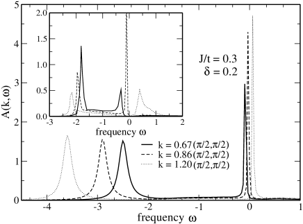
Figure 2: Solid, dashed, and doted lines are the spectral functions for ${\bf{k}}=0.67(\pi/2,\pi/2)$, ${\bf{k}}=0.86(\pi/2,\pi/2)$ and ${\bf{k}}=1.2(\pi/2,\pi/2)$ respectively. The frequency $\omega$ is in units of $t$ which is considered to be 1. For comparison with SB, in the inset we have included the results from Ref. KotliarS, .

In Fig. 2 we present PIH spectral functions $A({\bf{k}},\omega)$. The calculation was done for $J=0.3$, $\delta=0.20$ and for ${\bf{k}}=0.67(\pi/2,\pi/2)$, ${\bf{k}}=0.86(\pi/2,\pi/2)$ and ${\bf{k}}=1.2(\pi/2,\pi/2)$, which are exactly the same conditions of Fig. 3 in Ref. KotliarS, . In the inset of Fig. 2 we have included SB results for comparison. As can be seen, the spectral functions have some similarities with SB. We have obtained a low energy peak and a pronounced structure at large binding energy. The low energy peak is the quasiparticle (QP). The other features, at large binding energy, are incoherent spectra (IS). For ${\bf{k}}\sim 0.86(\pi/2,\pi/2)$ the QP peak crosses $\omega=0$, where the chemical potential is located. In spite of similarities between present results and those of Ref. KotliarS, there are some differences: a) Our IS is located at binding energy larger than in SB. For instance, for ${\bf{k}}=0.86(\pi/2,\pi/2)$, IS is at $\omega\sim-3t$ while the corresponding one in SB is at $\omega\sim-2t$. b) Our QP peak is less dispersing than in SB. As it is well known, self-energy effects depresses Fermi velocities ($v_{F}^{*}$) respect to the bare one ($v_{F}^{bare}$), $v_{F}^{*}=Zv_{F}^{bare}$, where $Z=(1-\frac{\partial\Sigma}{\partial\omega})$ is the QP weight therefore, it is concluded that our self-energy effects are larger than in SB.

In SB there are three different $\Sigma$’s KotliarS : $\Sigma_{n}$, $\Sigma_{a}$ and $\Sigma_{inc}$. In $\Sigma_{n}$, bosons are condensed, in $\Sigma_{a}$ one boson is condensed and the other fluctuates, and in $\Sigma_{inc}$ both bosons fluctuate. These complications are due to the decoupling scheme used in SB, so beyond mean field level it is necessary to convolute spinons and bosons for reconstructing the original $X$-operators. As in the PIH approach there is no any a priori decoupling and we work directly with the Hubbard operators, we have only one self-energy $\Sigma$ given by Eq. (17). A detailed description of the present self-energies for different $\delta$ and $J$ is given in section V.

After comparing spectral functions with some available SB results and, in spite of some similarities, we found important differences in the self-energy effects between both methods. The existence of only a few SB results beyond mean field level may be closely related to the decoupling scheme which leads to a gauge field theory, making hard the implementation of the approach. We hope that PIH be useful and a complement of the SB calculations.

IV Comparison with exact diagonalization

As pointed out in Sec. II, PIH approach weakens spin fluctuations over charge fluctuations. For instance, at leading order, while there are collective effects in the charge channel, the spin channel exhibits the characteristic form of a Pauli paramagnet where the electronic band is renormalized by correlations Lew ; Foussats1 . So that, at $O(1/N)$, the self-energy does not contain collective effects, like magnons in the spin channel. Intuitively one may think that the method will be better for large doping than for low doping. However, the exact role played by charge and magnetic excitations as a function of doping, in the $t-J$ model, is one of the key points for understanding the physics of cuprates. Many mechanisms have been proposed. Some of them privilege charge while others privilege magnetism.

In order to test the reliability of our results as a function of doping, in this section, we compare qualitatively present spectral functions with calculations obtained using Lanczos diagonalization. For this purpose we have performed Lanczos diagonalization Riera on the $4\times 4$ lattice for $\delta=0.75,\;0.5$ and $0.3125$, with $J=0.3$.

As an example, we will explicitly compare some ${\bf{k}}$-points for several dopings leaving to the reader the analysis of the other ${\bf{k}}$’s.

a) Results for doping $\delta=0.75$

This doping corresponds to $12$ holes in the $4\times 4$ lattice. There is good agreement between Lanczos and PIH (Fig. 3) for the six ${\bf{k}}$-points allowed in the $4\times 4$ lattice. For instance, for ${\bf{k}}=(0,\pi)$ both calculations show a QP peak at around $\omega\sim 2t$ and IS at around $\omega\sim-4t$. Lanczos diagonalization shows a small peak at $\omega\sim 3t$ which is not seen in PIH. However, PIH shows an asymmetric shape of the QP peak which can be interpreted as an indication of the additional structure observed in Lanczos. For ${\bf{k}}=(0,\pi/2)$ both, Lanczos and PIH show a QP peak near the Fermi level, and IS at $\omega\sim-4t$. The additional peak that appears in Lanczos at $\omega\sim 1.5t$ can be associated with the non-symmetrical shape of the QP peak seen in PIH.

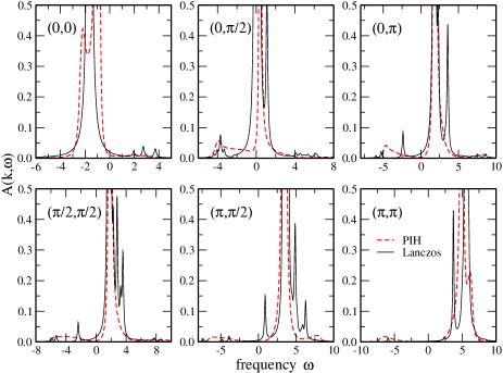
Figure 3: (Color online) Comparison between spectral function calculations obtained by Lanczos diagonalization for all the allowed ${\bf{k}}$-points of the $4\times 4$ lattice and results obtained with the PIH method. The parameters are $J=0.3$ and $\delta=0.75$. The ${\bf{k}}$-points are presented between parenthesis in each frame. The frequency $\omega$ is in units of $t$. In order to plot PIH and Lanczos results on the same figure we have used an arbitrary scale for the $y$-axis.

b) Results for doping $\delta=0.50$

This doping corresponds to $8$ holes in the $4\times 4$ lattice. Results are presented in Fig. 4 for Lanczos and PIH. With decreasing doping from $0.75$ to $0.50$, both methods show more IS. For instance, for ${\bf{k}}=(0,0)$ both calculations show two well defined peaks below the Fermi level. The peak closer to the chemical potential is the QP, and the peak near $\omega\sim-3t$ is of incoherent character. Both methods also present small IS for $\omega>0$.

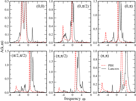
Figure 4: (Color online) Comparison between spectral function calculations obtained by Lanczos diagonalization for all the allowed ${\bf{k}}$-points of the $4\times 4$ lattice and results obtained with the PIH method. The parameters are $J=0.3$ and $\delta=0.5$. The ${\bf{k}}$-points are presented between parenthesis in each frame. The frequency $\omega$ is in units of $t$.

For $\delta=0.5$, results for $J=0$ were presented in Ref. Merino, in the context of organic materials where PIH spectral functions were also compared with those obtained using Lanczos diagonalization as a function of the nearest neighbors Coulomb interaction $V$.

c) Results for doping $\delta=0.3125$

This doping corresponds to $5$ holes in the $4\times 4$ lattice. The results are presented in Fig. 5 for Lanczos and PIH. Lanczos and PIH present the QP peak near the Fermi level and stronger IS than for $\delta=0.75$ and $\delta=0.5$. The increasing of the IS is consistent with the fact that the QP weight is $Z\sim 0.5$, lower than for the previous dopings where for $\delta=0.75$ and $\delta=0.5$ is $Z\sim 0.9$ and $Z\sim 0.7$ respectively. The QP weight will be discussed in more detail in next section.

For ${\bf{k}}=(0,0)$ both calculations show a QP peak below Fermi energy. The peak that appears in PIH at $\omega\sim-3t$ is broader in Lanczos and centered at $\omega\sim-4t$. For ${\bf{k}}=(\pi,\pi/2)$ both calculations show a QP peak above Fermi level and IS on the top of this peak. The well pronounced structure obtained in PIH at $\omega\sim-6t$ seems to be missing in Lanczos. Instead, it shows an homogeneously distributed IS below the Fermi level up to large binding energies of the order of $-7t$. In the frequency range $-5t<\omega<-1t$ both methods show IS. For ${\bf{k}}=(0,\pi)$ both methods present a QP near the Fermi level and IS at $\omega\sim-5t$. Between those two features it is possible to see IS (in the form of several peaks in Lanczos) in both calculations.

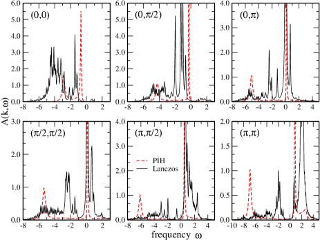
Figure 5: (Color online) Comparison between spectral function calculations obtained by Lanczos diagonalization for all the allowed ${\bf{k}}$-points of the $4\times 4$ lattice and results obtained with the PIH method. The parameters are $J=0.3$ and $\delta=0.3125$. The ${\bf{k}}$-points are presented between parenthesis in each frame. The frequency $\omega$ is in units of $t$.

For the three studied dopings both methods show that while the QP peak disperses through the Fermi surface (FS), the edge of the IS moves in opposite direction. This result was obtained previously by Stephan and HorschStephan . In Ref. Stephan, the authors also studied spectral functions for the $t-J$ model at moderate doping $\delta\sim 0.1$ by means of exact diagonalization. That paper presents strong evidences for a large FS for moderated doping levels. This result gives an additional support for our bare band $E_{k}=-2(t\;\delta/2+\Delta)(cos\,k_{x}+cos\;k_{y})-\mu$.

We conclude that PIH and Lanczos results, for the three studied $\delta$ values (which cover a broad range of doping), fairly agree considering the different nature of both methods. The above comparison gives some confidence to our self-energies. The self-energy has additional information such as relaxation times $1/\tau$, quasiparticle weight $Z$ (effective mass increasing) which can not be directly obtained from Lanczos diagonalization.

Decreasing doping , Lanczos and PIH both show band narrowing. The narrowing is stronger in PIH than in Lanczos. For instance, for $\bf{k}=(\pi,\pi)$ (Fig. 4), while the Lanczos QP peak is at $\omega\sim 4t$, the PIH QP peak is at $\omega\sim 2t$. For $\bf{k}=(\pi,\pi)$ (Fig. 5), while Lanczos QP peak is at $\omega\sim 2t$ it is at $\omega\sim 1t$ in PIH. For $\delta=0.75$ (Fig. 3) there is good agreement in the QP and IS energy positions for each $\bf{k}$. This discussion is important in the light of $ARPES$ experiments in cuprateszhou ; fink which show Fermi velocities rather independent of doping (see also Ref. Sorella, for discussions). In PIH the strong narrowing is mainly due to the factor $\delta/2$ in the electronic dispersion which strongly weakens the $t$-term.

V Self-energy renormalizations

In this section, we present a detailed self energy and spectral functions calculations from PIH.

Figure 6: Quasiparticle weight $Z$ as a function of doping for $J=0$.

Fig. 6 shows the QP weight $Z$ as a function of doping for $J=0$. As it was shown in Ref. Foussats1, , for $J=0$ the homogeneous Fermi liquid (HFL) remains stable for all $\delta$. For each doping, we have found that the self-energy is very isotropic on the FS (see below), making the QP weight rather constant. In Fig. 6 $Z\rightarrow 0$ when $\delta\rightarrow 0$. For small $\delta$, $Z\sim 1.4\;\delta$, which is very close to the observed $ARPES$ behavior in $LSCO$Yoshida . As $Z$ remains finite for $\delta>0$, present calculation predicts a Fermi liquid (FL) behaviour. Fig. 6 also shows that $Z\rightarrow 1$ when $\delta\rightarrow 1$ as expected for an uncorrelated system.

Figure 7: $-Im\Sigma({\bf{k_{F}}},\omega)$ (upper panel), $Re\Sigma({\bf{k_{F}}},\omega)$ (middle panel) and spectral functions (lower panel) for $J=0.3$, $\delta=0.30$ and three different points on the FS. Solid line, dashed line and dotted line are results for the Fermi point in the $(1,1)$, $(1,0)$ directions and between these two respectively. The frequency $\omega$, $Re\Sigma$ and $Im\Sigma$ are in units of $t$. Inset: $-Im\Sigma({\bf{k_{F}}},\omega)$ for ${\bf{k_{F}}}$ in the $(11)$-direction in units of $t=0.4eV$.

Let us discuss the case $J=0.3$. Fig. 7 shows $\Sigma$, for $\delta=0.3$, for three well separated ${\bf{k}}$-vectors on FS. One of the ${\bf{k}}$ is chosen in the $(11)$-direction of the BZ, other in the $(10)$-direction and the third in between both. The upper and the middle panel of Fig. 7 show the ${\mathrm{Im}}\Sigma$ and ${\mathrm{Re}}\Sigma$ respectively.

As shown in Fig. 7, PIH predicts a rather isotropic self-energy on the FS. On the other hand, for each ${\bf{k}}$, $\Sigma({\bf{k}},\omega)$ is very asymmetric respect to $\omega=0$ which can be interpreted as a consequence of the difference between addition and removal of a single electron in a correlated system. Near $\omega=0$, ${\mathrm{Im}}\Sigma({\bf{k}}_{F},\omega)\sim\omega^{2}$, showing FL behavior. On the other hand, ${\mathrm{Re}}\Sigma({\bf{k}}_{F},\omega)$ shows, at $\omega=0$, a negative slope which is also a characteristic of a Fermi liquid.

Inset of Fig. 7 shows a plot of $-{\mathrm{Im}}\Sigma({\bf{k_{F}}},\omega)$ for $\omega<0$ for ${\bf{k}}_{F}$ in the $(11)$-direction. We have used $t=0.4\;eV$ Reviwes . In the range $-200\;meV<\omega<0$, $-{\mathrm{Im}}\Sigma({\bf{k}},\omega)$ does not saturate as in Fig. 1 of Ref. zhou, . The no saturation of $-{\mathrm{Im}}\Sigma({\bf{k}},\omega)$, up to an energy scale of the order of $-200\;(-300)\;meV$, is well established in cuprates and clearly it can not be explained by phonons. In addition to this feature, Fig. 1 of Ref. zhou, shows the presence of an additional energy scale of the order of $60-70\;meV$ which is associated with the kink observed in $ARPES$ Reviwes . This small energy scale is not seen in our $-{\mathrm{Im}}\Sigma({\bf{k}},\omega)$. Whether the kink is due to magnetic excitations or additional degrees of freedom like phonons, is still controversial Reviwes ; Zeyher3 . For instance, Yunoki et  al. Sorella , using variational MC, found no evidence for the kink in the context of the pure $t-J$ model and, on the other hand, FLEX calculations for the Hubbard model suggest that the interaction between QP and spin fluctuations leads to the kink (see Ref. Manske, and references therein). As mentioned in previous sections the PIH approach weakens spin fluctuations over charge fluctuations, which means that $1/N^{2}$ self-energy corrections should be calculated in order to study the kink, if originated by magnetic excitations.

Finally, as expected from the results shown in the upper and middle panels, the lower panel of Fig. 7 shows that, for the three mentioned ${\bf{k}}$-vectors, the corresponding spectral functions are isotropic.

As it was shown in Ref. Foussats1, , in agreement with previous calculations Marston ; Lubenski ; Cappelluti , for $J=0.3$, the system presents a flux phase (FP) (also called $d$-density wave (DDW)Chakra ) for $\delta<\delta_{c}\sim 0.14$. FP was interpreted as a candidate for the pseudogap phase of cuprates Cappelluti ; Chakra . Thus, it is important to study self-energy corrections approaching the FP instability from the HFL phase ($\delta\rightarrow\delta_{c}$ from above). Similar calculations to those for $\delta=0.3$ show, for $\delta\gtrsim\delta_{c}\sim 0.14$, isotropic self-energy effects on the FS.

Figure 8: Quasiparticle weight $Z$ versus doping for the three ${\bf{k}}$-points on the FS discussed in Fig. 7. As discussed in the text there is no indication of the proximity to the DDW phase. The calculations run from $\delta>\delta_{c}\sim 0.14$ where the HFL is stable.

Fig. 8 shows $Z$ versus $\delta$ for three ${\bf{k}}$-points chosen as in Fig. 7; each one of them on its corresponding FS for each doping. Results are for $\delta<0.3$. The QP weight results very isotropic on the FS even for doping near $\delta_{c}$. According to our results the anisotropy, between $X$-point ($(10)$-direction) and nodal point ($(11)$-direction), observed in $ARPES$ spectra in cuprates, can not be interpreted as originated by self-energy effects. This is close to the recent interpretation by Kaminski et  al. Kami where the scattering rate was found to be composed by an isotropic inelastic term and a highly anisotropic elastic term which correlates with the anisotropy of the pseudogap. In our case, the ${\rm{Im}}\Sigma$ can be interpreted as the inelastic contribution to the scattering rate and the opening of the flux phase, which is mainly of static character Cappelluti ; Foussats1 , as the elastic term. (A close comparison with $ARPES$ experiments in cuprates, which needs a better FS as given by the $tt^{\prime}-J$ model, is in progress).

It is important to discuss the reason for the non strong influence of the flux instability on the self-energy. As discussed in Refs. Foussats1, , Cappelluti, , flux phase is mainly of static and $d$-wave symmetry character and it is weakly coupled to the charge sector. Being our self-energy dominated by charge fluctuations (see below), $\Sigma$ does not strongly prove the proximity to the DDW. In terms of Ref. Chakra, , the proximity to the DDW is hidden for the one-particle spectral densities. This is in contrast with the self-energy behaviour in the proximity of the usual charge density wave (CDW) instability. In Ref. Merino, it was shown that the QP weight $Z$ is strongly affected when the system approaches the CDW phase.

A discussion about the excitations that, interacting with electrons, cause the self-energy renormalizations is necessary. In the usual many body language, the self-energy can be expressed in terms of the relevant quantity $\alpha^{2}F(\omega)$Mahan , where the notation is chosen in a way such that $F(\omega)$ gives information on the density of states of a boson interacting with the electrons, and $\alpha^{2}$ about the coupling. In usual metals, $\alpha^{2}F(\omega)$ contains information of the electron-phonon interaction averaged over the FS. For simplicity, we will discuss the $J=0$ case. Eq. (23) is conveniently written for reading $\alpha^{2}F(\omega)$. In the first term of the second hand side of Eq. (23) we can interpret $B^{RR}=-2{\rm{Im}}D_{RR}$ as the spectral function of the boson mediating the interaction, while the remaining squared factor, $\Omega^{2}$, as the coupling. As discussed in Sec. II, $D_{RR}$ corresponds to the charge-charge correlation function (Eq. (9)).

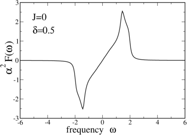
Figure 9: $\alpha^{2}F(\omega)$ as extracted from Eq. (23) for $\Sigma$. As discussed in the text, $\alpha^{2}F(\omega)$ is mainly dominated by collective excitations of the charge character. The frequency $\omega$ and $\alpha^{2}F$ are in units of $t$.

Fig. 9 shows $\alpha^{2}F(\omega)$ obtained from the first term of Eq. (17). Following the discussion above, $\alpha^{2}F(\omega)$ is proportional to the average on the FS of the charge densities. Clearly, charge densities survives up to high energy causing the large self-energy effects at large $\omega$. Since charge densities, in $O(1)$, present collective peaks at the top of the particle-hole continuumFoussats1 both, the collective excitations and the continuum, contribute to $\alpha^{2}F(\omega)$. For instance, the pronounced structure at $\omega\sim\pm 1.7$ in Fig. 9 is mainly due to collective fluctuations. The interpretation of the last two terms of the second hand side of Eq.(23) is less direct and they are proper of our strong coupling perturbative approach. However, they are also dominated by collective excitation of charge character arising from the inversion of the matrix $D$.

Sum rule: Before closing we will discuss the spectral function sum rule $\int d\omega\;A(\bf{k},\omega)$. In the framework of the $t-J$ model the sum rule is $<X^{00}>+<X^{\sigma\sigma}>=(1+\delta)/2$. Using the relation $X^{0\sigma}=\sqrt{Nr_{0}}\;f_{p}$, in the limit $N=2$, our sum rule is $\delta$ ($<X^{00}>$), therefore, PIH misses a contribution $<X^{\sigma\sigma}>=(1-\delta)/2$ making the situation better for large than for low doping. It is important to discuss about a possible origin of this discrepancy. As was pointed out in previous papers Foussats4 ; Foussats5 , in order to guarantee the commutation rules for $X$-operators not all the multiplication rules can be satisfied. For instance, in Ref. Foussats4, we have studied the spin system using the four $X$-operators $X^{\sigma\sigma^{\prime}}$ and showed that the formulation leads to the well known coherent state path integral representation for spinsFradkin . The fact that this representation is better for large than for small $S$ (Ref. Fradkin, ) was understood, in Ref. Foussats4, , as a consequence that not all the multiplication rules are fulfilled. It is worthy to note that the formalism in Ref. Foussats4, reproduces the spinless fermion case when they are written using $X$-operator representation. In the present case we deal with the $t-J$ model and in order to satisfy the commutation rules, the formalism requires the constraint $X^{\sigma 0}X^{0\sigma^{\prime}}=X^{00}X^{\sigma\sigma^{\prime}}$ Foussats ; Foussats5 which reproduces the exact multiplication rule $X^{\sigma 0}X^{0\sigma^{\prime}}=X^{\sigma\sigma^{\prime}}$ in the limit $X^{00}\rightarrow 1$ ($\delta\rightarrow 1$) making the representation better for large than for low doping. In mathematical terms, our expansion seems to be appropriate for both large $N$ and large $\delta$. This is closely related to the fact that the formulation weakens spin over charge fluctuations. The band narrowing, discussed in section IV, is possibly connected with this discussion if a spin term $<X^{\sigma\sigma}>$ also contributes to the bandwidth. The solution of this very hard theoretical problem, and the knowledge of how important it is as a function of doping on different physical quantities, requires not only to make an effort on formal level, but also, at the same time, confronting results with different methods.

VI Discussions and Conclusions

The recently developed path-integral large-$N$ approach for Hubbard operators, PIH, was used for calculating self-energy corrections and spectral functions, including fluctuations above mean field solution of the $t-J$ model.

Similarities and differences with SB were discussed in section III. To gain confidence on our calculation, comparisons of spectral functions with Lanczos results for $J=0.3$ and for doping $\delta=0.75$, $\delta=0.5$ and $\delta=0.3125$ were performed in section IV. We found fair agreement for each ${\bf{k}}$ on the BZ. PIH self-energies and spectral functions for different $J$ and $\delta$ have been investigated in Sec. V. The general characteristics of the self-energy are:

a) Around $\omega=0$, ${\rm{Im}}\Sigma(\omega)\sim\omega^{2}$ which is characteristic of a FL behavior. This is in agreement with the negative slope of ${\rm{Re}}\Sigma(\omega)$ at $\omega=0$.

b) $\Sigma(\omega)$ is very asymmetric with respect to $\omega=0$, indicating the difference between addition and removal of one electron in a strongly correlated system.

c) $\Sigma(\omega)$ has large structures at large negative $\omega$ of the order of a few $t$.

For $J=0$, we have shown that $Z$ decreases monotonically as $\delta\rightarrow 0$ remaining finite for $\delta>0$. For small $\delta$, $Z\sim 1.4\;\delta$. As expected, in the uncorrelated limit, $Z\rightarrow 1$ for $\delta\rightarrow 1$.

We have also studied spectral functions along the FS for different $\delta$ and $J=0.3$. For this case, the HFL is unstable against a DDW phase for doping $\delta<\delta_{c}\sim 0.14$. Since DDW phase was interpreted as a candidate for describing the pseudogap state in cuprates, we have studied the behavior of the self-energy along the FS when approaching the DDW instability. It has been found that self-energy effects and spectral functions are very isotropic along the FS even for doping close to $\delta_{c}$.

In Sec. V we have discussed the nature of the excitations, which interacting with the charge carriers produce the self-energy renormalizations. Charge excitations, dominated by collective effects, are the main contribution to $\alpha^{2}F(\omega)$. As collective charge fluctuations live on a large energy scale, they are the responsible for the large self-energy effects at large energy, producing the reduction of the quasiparticle weight and transferring spectral weight to the incoherent spectra at large binding energy.

PIH method seems to be a suitable alternative for calculating spectral functions in the $t-J$ model, moreover it can be used independently or as a complement to other calculations as well.

Acknowledgments

We thank L. Manuel, J. Merino, A. Muramatsu, A. Trumper and R. Zeyher for stimulating discussions and H. Parent for critical reading of the manuscript.

References

- (1) J.G. Bednorz and K.A. Müller, Zeit Phys. B 64, 189 (1986).
- (2) P.W. Anderson, The Theory of Superconductivity in High- Cuprates (Princeton University Press, Princeton, 1997).
- (3) A. Damascelli, Z-X. Shen and Z. Hussain, Rev. Mod. Phys. 75, 473 (2003).
- (4) G. Martinez and P. Horsch, Phys. Rev. B 44, 317 (1991).
- (5) A. Izyumov, Physics-Uspekhi 40, 445 (1997).
- (6) M. Brunner, F. Assaad and A. Muramatsu, Phys. Rev. B 62, 15480 (2000).
- (7) E. Dagotto, Rev. Mod. Phys. 66, 763 (1994).
- (8) J. Jaklic and P. Prelovsek, Adv. Phys. 49, 1 (2000).
- (9) A. Foussats and A. Greco, Phys. Rev. B 65, 195107 (2002).
- (10) E. Arrigoni, C. Castellani, M. Grilli, R. Raimondi and G. Strinati, Phys. Rep. 241, 291 (1994).
- (11) A. Foussats and A. Greco, Phys. Rev. B 70, 205123 (2004).
- (12) Z. Wang, Int. Journal of Modern Physics B 6, 155 (1992).
- (13) R. Zeyher and M. L. Kulić, Phys. Rev. B 53, 2850 (1996).
- (14) J. Merino, A. Greco, R. H. McKenzie, and M. Calandra, Phys. Rev. B 68, 245121 (2003).
- (15) A. Greco, J. Merino, A. Foussats and R. H. McKenzie, Phys. Rev. B 71, 144502 (2005).
- (16) Z. Wang, Y. Bang and G. Kotliar, Phys. Rev. Lett. 67, 2733 (1991).
- (17) L. Gehlhoff and R. Zeyher, Phys. Rev. B 52, 4635 (1995).
- (18) We thank J. Riera for usefull discussions and for his desinterested offer of his Lanczos programs.
- (19) W. Stephan and P. Horsch, Phys. Rev. Lett. 66, 2258 (1991).
- (20) X. J. Zhou, T. Yoshida, A. Lanzara, P. Bogdanov, S. Kellar, K. Sherr, W. Yang, F. Ronning, T. Sasagawa, T. Kakeshita, T. Noda, H. Eisaki, S. Uchida, C. Lin, F. Zhou, J. Xiong, W. Ti, Z. Zhao, A. Fujimori, Z. Hussain and Z.-X. Shen, Nature 423, 398 (2003).
- (21) J. Fink, S. Borisenko, A. Kordyuk, A. Koitzsch, J. Geck, V. Zabolotnyy, M. Knupfer, B. Büchner and H. Berger, cond-mat/0512307.
- (22) S. Yunoki, E. Dagotto and S. Sorella, Phys. Rev. Lett. 94, 037001 (2005)
- (23) T. Yoshida, X. Zhou, T. Sasagawa, W. Yang, P. Bogdanov, A. Lanzara, Z. Hussain, T. Mizokawa, A. Fujimori, H. Eisaki, Z.-X. Shen, T. Kakeshita and S. Uchida, Phys. Rev. Lett. 91, 027001 (2003).
- (24) R. Zeyher and A. Greco, Phys. Rev. B 64, 140510 (R) (2001).
- (25) D. Manske, The Theory of Unconventional Superconductors, (Springer-Verlag Berlin-Heidelberg, Germany 2004).
- (26) I. Affleck and J.B. Marston, Phys. Rev. B 37, 3774 (1988).
- (27) D.C. Morse and T.C. Lubensky, Phys. Rev. B 42, 7994 (1990).
- (28) E. Cappelluti and R. Zeyher, Phys. Rev. B 59, 6475 (1999).
- (29) S. Chakravarty, R. B. Laughlin, D. K. Morr, and Ch. Nayak, Phys. Rev. B 63, 94503 (2001).
- (30) A. Kaminski, H. Fretwell, M. Norman, M. Randeria, S. Rosenkranz, U. Chatterjee, J. Campuzano, J. Mesot, T. Sato, T. Takahashi, M. Takano, K. Kadowaki, Z. Li and H. Raffy, Phys. Rev. B 71, 014517 (2005).
- (31) G. Mahan, Many-Particle Physics (Plenum Press, New York, 1981).
- (32) A. Foussats, A. Greco and O. S. Zandron, Ann. Phys. (N.Y.) 275, 238 (1999); 279, 263 (2000).
- (33) A. Foussats, A. Greco, C. Repetto, O. P. Zandron and O. S. Zandron, Journal of Physics A 33, 5849 (2000).
- (34) E. Fradkin, Field Theories of Condensed Matter Systems (Addison-Wesley, Reading, Massachusetts, 1991).