Current-driven destabilization of both collinear configurations in asymmetric spin-valves

Abstract

Spin transfer torque in spin valves usually destabilizes one of the collinear configurations (either parallel or antiparallel) and stabilizes the second one. Apart from this, balance of the spin-transfer and damping torques can lead to steady precessional modes. In this letter we show that in some asymmetric nanopillars spin current can destabilize both parallel and antiparallel configurations. As a result, stationary precessional modes can occur at zero magnetic field. The corresponding phase diagram as well as frequencies of the precessional modes have been calculated in the framework of macrospin model. The relevant spin transfer torque has been calculated in terms of the macroscopic model based on spin diffusion equations.

Introduction: Spin transfer between conduction electron system and localized magnetic moments gives rise to new phenomena, like for instance current-induced switching between different magnetic states Slonczewski96 . Several theoretical models have been developed to describe physical mechanisms of the spin transfer and magnetic switching phenomena Stiles02 ; Brataas01 ; weintal00 ; zhang02 ; Barnas05 . Apart from this, magnetic switching has been observed in a number of experiments Katine00 ; grolier01 ; darwish04 ; tsoi04 .

At certain conditions electric current can cause transition to steady precessional modes, where the energy is pumped from conduction electrons to localized magnetic moments Slavin05 ; Sun00Li03 ; Kiselev0305 ; Rippard04 ; Xi04 ; Xiao05 . This phenomenon is of high importance due to possible applications in microwave generation. In typical Co/Cu/Co spin valves, the steady precessions exist for external magnetic fields larger than the anisotropy field, and for currents exceeding certain critical values Kiselev0305 ; Rippard04 . For lower values of external field, the current drives switching to antiparallel (AP) or parallel (P) states, depending on the initial state of the system.

In this Letter we show that spin transfer torque in asymmetric systems (with the two magnetic films having different bulk and interface spin asymmetry factors, e.g., Co/Cu/Py nanopillars) vanishes at a certain noncollinear configuration due to an inverse spin accumulation in the nonmagnetic spacer layer. As a result, spin current can destabilize both P and AP magnetic configurations for one orientation of the bias current and stabilize both configurations for the opposite current. The former case is of particular interest, as the spin current can excite precessional modes in the absence of external magnetic field, which is of particular importance from the application point of view. Such a system is thoroughly studied in this Letter.

Model and description: We consider a tri-layer system which is attached to two external nonmagnetic leads. The tri-layer consists of a magnetically fixed (thick) layer of thickness $d_{1}$, nonmagnetic spacer layer of thickness $d_{2}$, and a thin magnetic (free or sensing) layer of thickness $d_{3}$. Magnetic dynamics of the sensing layer is described by the generalized Landau-Lifshitz-Gilbert equation

$$\frac{{\rm d}\hat{\bm{s}}}{{\rm d}t}=-|\gamma_{\rm g}|\mu_{0}\,\hat{\bm{s}}\times{\bm{H}}_{\rm eff}-\alpha\,\hat{\bm{s}}\times\frac{{\rm d}\hat{\bm{s}}}{{\rm d}t}+\frac{|\gamma_{\rm g}|}{M_{\rm s}d_{3}}\,\bm{\tau}\,,$$ (1)

where $\hat{\bm{s}}$ is the unit vector along the spin moment of the sensing layer, $\gamma_{\rm g}$ is the gyromagnetic ratio, $\mu_{0}$ is the magnetic vacuum permeability, ${\bm{H}}_{\rm eff}$ is an effective magnetic field acting on the sensing layer, $\alpha$ is the damping parameter, and $M_{\rm s}$ stands for the saturation magnetization. Generally, the effective field includes an external magnetic field $H_{\rm ext}$, the uniaxial magnetic anisotropy field $H_{\rm a}$, and the demagnetization field $H_{\rm d}$; ${\bm{H}}_{\rm eff}=-H_{\rm ext}\,\hat{\bm{e}}_{\rm z}-H_{\rm a}(\hat{\bm{s}}\cdot\hat{\bm{e}}_{z})\,\hat{\bm{e}}_{z}+H_{\rm d}(\hat{\bm{s}}\cdot\hat{\bm{e}}_{x})\,\hat{\bm{e}}_{x}$, where $\hat{\bm{e}}_{x}$ and $\hat{\bm{e}}_{z}$ are the unit vectors along the axes $x$ (normal to the layers) and $z$ (in-plane), respectively. The last term in Eq.(1) stands for the torque due to spin transfer, $\bm{\tau}=\bm{\tau}_{\theta}+\bm{\tau}_{\varphi}$, with $\bm{\tau}_{\theta}=aI\,\hat{\bm{s}}\times(\hat{\bm{s}}\times\hat{\bm{S}})=\tau_{\theta}\hat{\bm{e}}_{\theta}$, and $\bm{\tau}_{\varphi}=bI\,\hat{\bm{s}}\times\hat{\bm{S}}=\tau_{\varphi}\hat{\bm{e}}_{\varphi}$. Here, $\hat{\bm{S}}$ is the unit vector along the spin moment of the fixed magnetic layer ($\hat{\bm{S}}=\hat{\bm{e}}_{z}$), while $\hat{\bm{e}}_{\theta}$ and $\hat{\bm{e}}_{\varphi}$ are the unit vectors of a coordinate system associated with the polar $\theta$ and azimuthal $\varphi$ angles describing orientation of the vector $\hat{\bm{s}}$. The current $I$ is defined as positive when it flows from the sensing layer towards the thick magnetic one (opposite to the axis $x$).

The current-induced torque $\bm{\tau}$ and the corresponding parameters $a$ and $b$ have been calculated in the diffusive transport regime, assuming that the spin current component perpendicular to the spin moment of the sensing layer is entirely absorbed in the interfacial region Stiles02 ; Brataas01 ; Barnas05 . For the parameter $a$ one then finds Barnas05

$$a=\frac{\hbar}{e^{2}}\bigg{[}{\rm Re}\{G_{\uparrow\downarrow}\}\bigg{(}\cot\theta(\tilde{g}_{x}\cos\varphi+\tilde{g}_{y}\sin\varphi)-\tilde{g}_{z}\bigg{)}$$

$$+\frac{{\rm Im}\{G_{\uparrow\downarrow}\}}{\sin\theta}\bigg{(}\tilde{g}_{x}\sin\varphi-\tilde{g}_{y}\cos\varphi\bigg{)}\bigg{]}\bigg{|}_{x\to x_{0}^{-}}\,,\,\,\,$$ (2)

where $\tilde{\bf g}={\bf g}/I$, with the spin accumulation components ${\bf g}=(g_{x},g_{y},g_{z})$ taken in the nonmagnetic spacer at the very interface with the sensing layer $(x\to x_{0}^{-})$, and $G_{\uparrow\downarrow}$ is the mixing conductance Brataas01 . The parameter $b$ is given by a similar formula, but with ${\rm Re}\{G_{\uparrow\downarrow}\}$ replaced by $-{\rm Im}\{G_{\uparrow\downarrow}\}$ and ${\rm Im}\{G_{\uparrow\downarrow}\}$ replaced by ${\rm Re}\{G_{\uparrow\downarrow}\}$.

A qualitative picture of the non-linear dynamics can be obtained from the local phase portraits of the corresponding linearized system in the vicinity of fixed points. Accordingly, we linearized Eqs.(1) and calculated eigenvalues of the corresponding Jacobian. For a two dimensional problem (as in our case) the eigenvalues depend only on the trace and determinant of the Jacobian. Apart from this, the eigenvalues are current dependent and determine stability of the fixed points. More specifically, the point is stable when real parts of all the eigenvalues are negative, and becomes unstable when at least one of them is positive. The system considered, Eqs.(1), can have several fixed points given by $\bm{\tau}=\mu_{0}M_{\rm s}d_{3}\hat{\bm{s}}\times{\bm{H}}_{\rm eff}$. However, only two of them, P and AP, are trivial with position independent of current. In addition, the current driven global phase portrait of the system considered below contains two saddle points with separatrices dividing the phase space to basin of attraction for P and AP fixed points and two focuses (located near energy maximum).

Critical currents: Consider first the P state and assume positive determinant of the corresponding Jacobian. Since the eigenvalues of the linearized problem can be complex numbers, the non-zero imaginary parts give rise to periodic components of the fundamental solutions. The condition of vanishing trace determines the critical current $I_{\rm c}^{\rm PRC}$ which destabilizes the P state and switches system to a precessional (PRC) state (this can be assign as Hopf bifurcation with a limit cycle emerging),

$$I_{\rm c}^{\rm PRC}=\frac{\alpha\mu_{0}M_{\rm s}d_{3}}{a-b\,\alpha}\left(H_{\rm a}+H_{\rm ext}+\frac{H_{\rm d}}{2}\right)\bigg{|}_{\theta\to 0}\,,$$ (3)

where the parameters $a$ and $b$ have to be calculated in the limit of $\theta\to 0$. With a further increase in current, the complex conjugated imaginary parts of the eigenvalues vanish at a certain point, at which two real eigenvalue branches arise. When current increases further, one of the eigenvalues goes to zero, leading to a saddle-node bifurcation. In the case studied below, two new saddles appear inside the limit cycle making it unstable wiggins . Thus, the critical currents driving system to a static state (SS) can be found as,

$$I_{{\rm c}\pm}^{\rm SS}=-\frac{\mu_{0}M_{\rm s}d_{3}}{a^{2}+b^{2}}\bigg{[}b\left(H_{\rm a}+H_{\rm ext}+\frac{H_{\rm d}}{2}\right)\qquad$$ (4)

$$\pm\frac{1}{2}\sqrt{b^{2}H_{\rm d}^{2}-4a^{2}(H_{\rm a}+H_{\rm ext})(H_{\rm a}+H_{\rm ext}+H_{\rm d})}\bigg{]}\bigg{|}_{\theta\to 0}\,.$$

The signs of critical currents depend on the parameters $a$ and $b$ taken at $\theta\rightarrow 0$. In the case considered below, $I>0$, these parameters obey the conditions $a-b\alpha>0$ and $b<0$ (the following discussion is limited to the case, where these conditions are fulfilled). Consequently, the PRC regime holds for $I>I_{\rm c}^{\rm PRC}$, and the P state is stable for $I<I_{\rm c}^{\rm PRC}$. Since $I_{{\rm c}+}^{\rm SS}<I_{{\rm c}-}^{\rm SS}$, the SS states can occur for $I>I_{{\rm c}+}^{\rm SS}$, and we can skip $I_{{\rm c}-}^{\rm SS}$ in the following considerations.

Asymmetric nanopillars: Let us consider now an asymmetric nanopillar, where the two ferromagnets and/or two external leads are of different materials, like for instance Cu/Co/Cu/Py/Cu spin valve. It has been predicted recently that the spin-transfer torque acting on the sensing layer in such a spin valve can vanish for a noncollinear magnetic configuration Barnas05 . In Fig.1(b,c) we plot the angular variation of the torques $\tau_{\varphi}$ and $\tau_{\theta}$, which clearly shows that $\tau_{\theta}$ vanishes at $\theta_{c}\neq 0,\pi$. Such a behavior of $\tau_{\theta}$ can be observed if an inverse spin accumulation builds up in the spacer layer, as shown schematically in Fig.1(a). This can be achieved when the fixed magnetic layer has bulk spin asymmetry weaker than that of the sensing layer, and its thickness is smaller than the spin diffusion length.

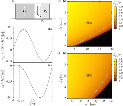
Figure 1: (color online) (a) Schematic structure of the nanopillar and spin accumulation in thin spacer layer for the parallel configuration of the magnetic layers, and for electrons flowing along the axis $x$. Angular dependence of the torques $\tau_{\varphi}$ (b) and $\tau_{\theta}$ (c), acting on the Py layer in the Cu/Co(10)/Cu(10)/Py(4)/Cu spin valve (independent of $\varphi$). (d) $\theta_{\rm c}/\pi$ as a function of $d_{1}$ and $d_{3}$ in the nanopillar Cu/Co($d_{1}$)/Cu(10)/Py($d_{3}$)/Cu. The white dashed line corresponds to a critical thicknesses for ZFOs (zero-field oscillations). (e) $\theta_{\rm c}/\pi$ in the Cu/Co($d_{1}$)/Cu(10)/Py($d_{3}$)/Au structure. The other parameters are: (Co) bulk resistivity $\rho^{*}=5.1\,{\rm\mu\Omega cm}$, spin asymmetry factor $\beta=0.51$, and spin-flip length $l_{\rm sf}=60\,{\rm nm}$; (Py) $\rho^{*}=16\,{\rm\mu\Omega cm}$, $\beta=0.77$, $l_{\rm sf}=5.5\,{\rm nm}$; (Cu) $\rho^{*}=0.5\,{\rm\mu\Omega cm}$, $l_{\rm sf}=1000\,{\rm nm}$; (Au) $\rho^{*}=2\,{\rm\mu\Omega cm}$ and $l_{\rm sf}=60\,{\rm nm}$. In turn, for the Co/Cu interfaces we assume the interfacial resistance per unit square $R^{*}=0.52\times 10^{-15}\,{\rm\Omega m^{2}}$, interface spin asymmetry factor $\gamma=0.76$, and the mixing conductances ${\rm Re}\{G_{\uparrow\downarrow}\}=0.542\times 10^{15}\,{\rm\Omega^{-1}m^{-2}}$, and ${\rm Im}\{G_{\uparrow\downarrow}\}=0.016\times 10^{15}\,{\rm\Omega^{-1}m^{-2}}$; for the Py/Cu interfaces we assume $R^{*}=0.5\times 10^{-15}\,{\rm\Omega m^{2}}$, $\gamma=0.7$, ${\rm Re}\{G_{\uparrow\downarrow}\}=0.39\times 10^{15}\,{\rm\Omega^{-1}m^{-2}}$, and ${\rm Im}\{G_{\uparrow\downarrow}\}=0.012\times 10^{15}\,{\rm\Omega^{-1}m^{-2}}$.

The general conditions for vanishing spin torque at a noncollinear configuration can be derived assuming $\partial\tau_{\theta}/\partial\theta>0$ in both P and AP states, and for in-plane configurations ($\varphi\to\pi/2$) it has the form

$$\left(\pm{\tilde{g}}_{z}-\frac{{\rm Im}\{G_{\uparrow\downarrow}\}}{{\rm Re}\{G_{\uparrow\downarrow}\}}\frac{\partial{\tilde{g}}_{x}}{\partial\theta}\mp\frac{\partial{\tilde{g}}_{y}}{\partial\theta}\right)\Bigg{|}_{\scriptsize\begin{array}[]{l}\theta\to 0\\[-2.0pt] \theta\to\pi\end{array}}<0\,.$$ (5)

For a general configuration one has to replace ${\tilde{g}}_{x}\mapsto({\tilde{g}}_{x}\sin\varphi-{\tilde{g}}_{y}\cos\varphi)$ and ${\tilde{g}}_{y}\mapsto({\tilde{g}}_{x}\cos\varphi+{\tilde{g}}_{y}\sin\varphi)$.

The parameter $\theta_{\rm c}/\pi$ is plotted in Fig.1 as a function of $d_{1}$ and $d_{3}$ for the right lead made of Cu (d) and Au (e), respectively. As one can note, $\theta_{\rm c}$ becomes particularly large for thin Co layers and thick Py ones. However, for a too large ratio $d_{3}/d_{1}$ the roles of the Co layer as a fixed one and Py as a sensing layer could be interchanged. Therefore, in the following we will consider the Cu/Co(10)/Cu(10)/Py(4)/Cu nanopillar (the numbers are the layer thicknesses in nanometers), with Py as a sensing layer and Co as the magnetically fixed one. For the Py layer we assume $M_{\rm s}=10053.1\,{\rm Oe}$, $H_{\rm a}=2.51\,{\rm Oe}$, $H_{\rm d}=0.65M_{\rm s}$ and $\alpha=0.003$. The dependence of $\theta_{\rm c}$ on the spacer thickness is rather weak, so thicker spacers can be used to eliminate possible interlayer exchange interaction. From comparison of Figs 1(d) and 1(e) follows that reducing the spin-flip length in the lead adjacent to the sensing layer increases $\theta_{\rm c}$ and also enhances the torque acting on the free layer (reducing the relevant critical current). This is due to an increased spin accumulation at the Cu/Py interface. The $\tau_{\varphi}$ component is usually much smaller than $\tau_{\theta}$, and therefore plays a negligible role in the initial stage of the switching from P state.

From the above follows that in asymmetric spin valves both P and AP states can be unstable when current density exceeds a certain critical value. Accordingly, precessional states and/or bistability of the static states can be expected for certain values of spin current Slavin05 ; Sun00Li03 ; Xi04 . If energy of a static state is close to the magnetic energy maximum, and a critical current for its stabilization is larger than the critical current needed to destabilize the state corresponding to the energy minimum, the PRC state is allowed Slavin05 . Thus, the sufficient condition for the presence of oscillations reads $I_{\rm c}^{\rm SS}>I_{\rm c}^{\rm PRC}$. The above condition, together with the necessary condition of vanishing spin torque in a noncollinear configuration, allow us to determine the region where the zero-field oscillations (ZFOs) exist. In Fig.1(d-e), the white dashed lines (corresponding to $I_{\rm c}^{\rm SS}=I_{\rm c}^{\rm PRC}$) separate the regions where the ZFOs occur from those where they cannot exist. We note that critical currents for switching from the AP state are still given by Eqs (3) and (4), but with r.h.s. multiplied by $-1$ and $H_{\rm ext}$ replaced by $-H_{\rm ext}$.

Figure 2 shows dynamical phase diagram of the Cu/Co/Cu/Py/Cu nanopillar. The reduced magnetoresistance, $r=(1-\cos^{2}(\theta/2))/(1+\cos^{2}(\theta/2))$, is shown there as a function of the external field and reduced current density $I/I_{0}$, with $I_{0}=10^{8}\,{\rm Acm^{-2}}$. The dashed lines correspond to the critical currents given by the analytical formulas (3) and (4), and fit very well to the numerical results. For weak external fields we find a stable static state with a high magnetoresistance value (HSS), which is close to maximal magnetic energy.

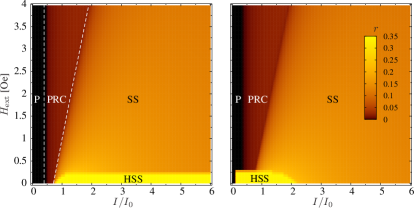
Figure 2: (color online) Dynamical phase diagram of the magnetoresistance for the Cu/Co(10)/Cu(10)/Py(4)/Cu spin valve, scanned by increasing (left) and decreasing (right) current with the sweeping rate $59$ A/cm²s in a constant applied field. The dashed lines correspond to critical currents given by Eqs (3) and (4). The other parameters as in Fig.1.

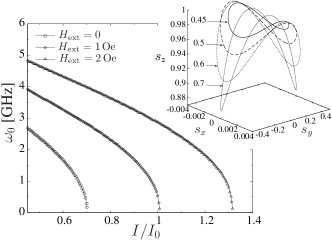
Figure 3: Fundamental frequency of the magnetoresistance oscillations in Cu/Co(10)/Cu(10)/Py(4)/Cu, calculated as a function of the reduced current swept with the rate $16$ A/cm²s in a constant external field as indicated. The inset shows precession orbits in zero external magnetic field for $I/I_{0}=0.45,0.5,0.6,0.7$. The other parameters as in Fig.1.

The microwave oscillations exist in the area between the two dashed white lines in Fig.2.(left part). As one can see, these oscillations exist in the absence of magnetic field for a certain current region. The fundamental frequency $\omega_{0}$ (first harmonics) of the magnetoresistance oscillations is shown in Fig.3 as a function of the current density and for different magnetic fields. Along the segments, where $\hat{\bm{s}}$ moves almost in the layer plane, the spin precesses mainly around $H_{\rm a}$ and $H_{\rm ext}$, with the angular velocity proportional to $|\gamma_{\rm g}|(H_{\rm a}+H_{\rm ext})$, see the inset in Fig.3. Along the remaining part ($\hat{\bm{s}}$ moves almost perpendicularly to the layer plane), the angular velocity is larger and proportional to $|\gamma_{\rm g}|(H_{\rm a}+H_{\rm ext}+H_{\rm d})$. With increasing $I$, the average orbital speed decreases while the arc length of the orbit increases. Consequently, $\omega_{0}$ decreases with increasing $I$.

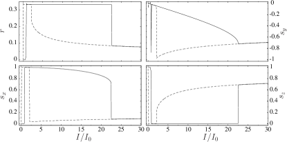
Figure 4: Current driven hysteretic behavior of the magnetoresistance and spin components of the sensing layer in zero field, scanned with increasing (solid line) and decreasing (dashed line) current with the sweeping rate $140$ A/cm²s. The parameters as in Fig.2.

Such precessions of decreasing frequency with increasing current in symmetrical spin valves are called ’clamshell’Kiselev0305 or ’in-plane’Xiao05 modes. But the main difference between symmetrical pillars and those studied in this Letter concerns the way the spin transfer acts on $\hat{\bm{s}}$. In our case, increasing current leads to an increase in $\bm{\tau}$, and the orbits become narrower and elongated in the $z$ direction due to $\bm{\tau}_{\theta}$. At the critical current density given by Eq.(4), when $s_{z}=\cos\theta_{\rm c}$, $\tau_{\theta}$ vanishes and orbital velocity reaches minimum. The damping torque is small, and the orbit bifurcates into SS states (fixed points) due to a non-zero $\tau_{\varphi}$. A further current increase at low fields drives the system via a transient regime to HSS state with positive or negative $s_{x}$ component (see Fig.4). The presence of HSS states gives rise to a current-driven hysteresis (Figs.2 and 4). The hysteresis for lower fields can be formally written as a sequence of transitions P$\to$PRC$\to$SS$\to$${\rm T_{+}}$$\to$HSS$\to$${\rm T_{-}}$$\to$SS for increasing current and SS$\to$${\rm T_{+}}$$\to$HSS$\to$${\rm T_{-}}$$\to$OOP$\to$P/AP for the decreasing current, with final bistability reached via the ’out-of-plane’ precessions (OOP), observed also in symmetrical spin-valves Xiao05 . The switching from SS state to a HSS state is mediated by the transient regime ${\rm T_{+}}$ (where spin transfer pumps energy to the system). The HSS states can be observed in a quite broad region, up to $I/I_{0}\simeq 22.5$, and further current increase switches system via the next transient ${\rm T_{-}}$ regime (where spin transfer dissipates energy) to the SS state. For higher fields the HSS states become unstable and the hysteresis vanishes. Finally we note that for $\tau_{\varphi}=0$ the static states will not occur and the area of PRC states extends for $I>I_{\rm c}^{\rm PRC}$.

In conclusion, we have shown that spin polarized current in certain asymmetrical structures can destabilize both P and AP configurations of a nanopillar spin-valve, and drive microwave oscillations in the absence of magnetic field. This takes place only for one orientation of the bias current. We have also presented the corresponding dynamical phase diagram.

Acknowledgements We thank A. Fert and D. Horváth for useful discussions. This work is partly supported by Slovak Grant Agencies APVT-51-052702, VEGA 1/2009/05, and by EU through RTN Spintronics (HPRN-CT-2000-000302).

References

- (1) J. C. Slonczewski, J. Magn. Magn. Mater. 159, L1 (1996); 195, L261 (1999); L. Berger, Phys. Rev. B 54, 9353 (1996).
- (2) M. D. Stiles and A. Zangwill, Phys. Rev. B 66, 014407 (2002).
- (3) A. Brataas, Yu. V. Nazarov, G. E. W. Bauer, Eur. Phys. J. B 22, 99, (2001).
- (4) X. Waintal, E. B. Myers, P. W. Brouwer, and D. C. Ralph, Phys. Rev. B 62, 12317 (2000); Y. B. Bazaliy, B. A. Jones, and S. C. Zhang, Phys. Rev. B 57, R3213 (1998).
- (5) S. Zhang, P. M. Levy, and A. Fert, Phys. Rev. Lett. 88, 236601 (2002); A. Shpiro, P. M. Levy, and S. Zhang, Phys. Rev. B 67, 104430 (2003).
- (6) J. Barnaś, A. Fert, M. Gmitra, I. Weymann, V. K. Dugaev, Phys. Rev. B 72, 024426 (2005); Mater. Sci. Eng. B 126, 271 (2006)
- (7) J. A. Katine, F. J. Albert, R. A. Buhrman, E. B. Myers, and D. C. Ralph, Phys. Rev. Lett. 84, 3149 (2000).
- (8) J. Grollier, V. Cros, A. Hamzic, J. M. George, H. Jaffres, A. Fert, G. Faini, J. Ben Youssef, and H. Legall, Appl. Phys. Lett. 78, 3663 (2001).
- (9) M. AlHajDarwish, H. Kurt, S. Urazhdin, A. Fert, R. Loloee, W. P. Pratt, Jr., and J. Bass, Phys. Rev. Lett. 93, 157203 (2004).
- (10) M. Tsoi, J. Z. Sun, M. J. Rooks, R. H. Koch, and S. S. P. Parkin, Phys. Rev. B 69, 100406(R) (2004).
- (11) A. N. Slavin, V. S. Tiberkevich, Phys. Rev. B 72, 094428 (2005).
- (12) J. Z. Sun, Phys. Rev. B 62, 570 (2000); Z. Li, S. Zhang, Phys. Rev. B 68, 024404 (2003).
- (13) S. I. Kiselev, J. C. Sankey, I. N. Krivorotov, N. C. Emley, R. J. Schoelkopf, R. A. Buhrman, D. C. Ralph, Nature (London) 425, 380 (2003).
- (14) W. H. Rippard, M. R. Pufall, S. Kaka, S. E. Russek, T. J. Silva, Phys. Rev. Lett. 92, 027201 (2004).
- (15) H. Xi, Z. Lin, Phys. Rev. B 70, 092403 (2004).
- (16) J. Xiao, A. Zangwill, and M. D. Stiles, Phys. Rev. B 72, 014446 (2005).
- (17) S. Wiggins, Introduction to Applied Nonlinear Dynamical Systems and Chaos, (Springer, New York 1990).