Identifying reactive trajectories using a moving transition state

Abstract

A time-dependent no-recrossing dividing surface is shown to lead to a new criterion for identifying reactive trajectories well before they are evolved to infinite time. Numerical dynamics simulations of a dissipative anharmonic two-dimensional system confirm the efficiency of this approach. The results are compared to the standard fixed transition state dividing surface that is well-known to suffer from recrossings and therefore requires trajectories to be evolved over a long time interval before they can reliably be classified as reactive or non-reactive. The moving dividing surface can be used to identify reactive trajectories in harmonic or moderately anharmonic systems with considerably lower numerical effort or even without any simulation at all.

I Introduction

It is perhaps surprising how many problems in chemistry, physics, and biology can be reduced to the simple model of diffusion over a barrier Talkner and Hänggi (1995). Although chemical reactions in all phases of matter provide the prime example Miller (1998); G.Truhlar et al. (1996), a plethora of systems that evolve from suitably defined “reactant” to “product” states are amenable to a description in this framework Jaffé et al. (2002); Koon et al. (2000); Komatsuzaki and Berry (2002); JFU ; Eckhardt (1995); Toller et al. (1985). Transition State Theory (TST) Truhlar et al. (1985); Hänggi et al. (1990); G.Truhlar et al. (1996) or one of its descendants Grote and Hynes (1980); Pollak et al. (1989); Mel’nikov and Meshkov (1986) is often used to approximate the rate of these reaction processes. This theory is based on the assumption that the reaction rate is determined in a small volume of the phase space near the barrier. It is then possible to define a dividing surface separating reactants from products and obtain the rate from the flux through this surface. The optimal location of the dividing surface is that which minimizes the number of recrossings—the fundamental idea of variational transition state theory Truhlar and Garrett (1984); Pollak (1990, 1992); Tucker and Pollak (1992); Tucker (1995). When the system of interest can be viewed as isolated from its environment, as in low-density gas phase chemical reactions, TST may indeed provide an excellent approximation to the rate. However, most processes of interest do not take place in isolation, but rather in a complex environment where interactions between the system and its surroundings occur on time scales comparable to that of the reaction: In a reaction occurring in the condensed phase, for instance, the dynamics of the solute is strongly coupled to that of the solvent. In this case, the fundamental assumption of TST, that the dividing surface is crossed once and only once, no longer holds Straub et al. (1985, 1986, 1988); Pollak and Talkner (1995). On the time scale of the reaction event, fluctuations of the environment will almost inevitably cause recrossings of the dividing surface that lead to an overestimation of the rate.

To overcome the recrossing problem, many TS dividing surfaces have been suggested in the literature Hynes (1985); G.Truhlar et al. (1996); Pollak (1986); Tucker (1995) which provide systematic (and simple) approximations to the optimal TS dividing surface. In some cases, the dividing surface has been identified in the infinite-dimensional phase space consisting of the system and an explicit set of bath oscillators Zwanzig (1973); Caldeira and Leggett (1981); Pollak (1986). This approach leads to an excellent approximation to the rate Pollak (1986); Pollak et al. (1989). Interestingly, the same result was subsequently obtained without recourse to the explicit heat bath model, using instead a collective reaction coordinate containing the influence of the bath directly Graham (1990).

In a recent series of papers Bartsch et al. (2005a, b), we reformulated the recrossing problem using a dividing surface that is itself moving stochastically so as to avoid recrossings. The motion of that surface follows the unique trajectory —named the TS trajectory— that never leaves the barrier region. Any reactive trajectory crosses the moving surface once and only once, whereas a nonreactive trajectory does not cross at all. This construction extends the approach of Graham (1990) in that it provides not only a reaction coordinate, but also the complete geometric structure by specifying all of the unstable and stable degrees of freedom globally Martens (2002). The previous purely analytic studies Bartsch et al. (2005a, b) are complemented here with a numerical investigation of the reaction dynamics for a two-dimensional stochastic nonlinear model. It will be shown that the moving dividing surface offers considerable computational advantages over the traditional fixed surface: Its use can significantly reduce the simulation time required to distinguish between reactive and nonreactive trajectories. Indeed, for a harmonic barrier it identifies reactive trajectories a priori, so that the need to simulate their dynamics does not arise at all. In an anharmonic system, the identification of reactive trajectories by the moving surface is no longer exact. Nevertheless, for moderately strong anharmonicities it provides a useful approximation, and its advantages over the fixed surface are retained. In addition, the moving TS surface introduces novel observables that characterize the reaction process on a microscopic level. Most prominently, it allows one to define a unique reaction time for each individual trajectory.

The outline of this paper is as follows: In Sec. II, the two-dimensional stochastic nonlinear model that is the focus of the computational studies in this work is defined and the construction of the moving TS dividing surface and its associated geometric structures is briefly reviewed. In Sec. III, the ensemble of trajectories is specified by a thermal distribution of particles localized at the conventional TST dividing surface. This barrier ensemble is reminiscent of the weighting distribution in standard rate expressions and is appropriate even in nonlinear cases. Its simple structure also readily leads to the analytic determination of several observables of the model system in the harmonic limit (Sec. IV). They are in precise agreement with the numerical results presented in Sec. V. The latter section also demonstrates that observables converge faster when evaluated using the moving dividing surface rather than conventional numerical methods, both in the harmonic limit and in systems with anharmonic barriers. This observation is particularly useful in the anharmonic case when the chosen system is not amenable to analytic approaches.

II Preliminaries

Although the general theory is applicable to systems with an arbitrary number $n$ of degrees of freedom, the following discussion will be restricted to $n=2$ coordinates under the influence of a stochastic bath. This choice can be made without loss of generality because it exhibits all the salient features of the higher-dimensional cases: It can encompass an unbound (reactive) direction and a bound bath mode whose interaction with the reactive mode is strong enough to require its explicit description. The coupling of the modes is described by a Taylor expansion about a transition point (or col) on the potential energy surface. Such a model with a minimum number of nonlinear terms is described in this section. It will be used in the following to study the effect of increasing anharmonicity on the identification of reactive trajectories.

To set the stage for the following investigations, the construction of the moving TST dividing surface and the associated invariant manifolds is summarized in the remainder of this section. The reader interested in a full exposition is referred to Refs. Bartsch et al., 2005a and Bartsch et al., 2005b, where the formalism was first introduced.

II.1 The Two-Dimensional Dissipative Model

A prototypical reactive system within a solvent may be described by the Langevin equation Zwanzig (2001)

$$\ddot{\vec{q}}_{\alpha}(t)=-\nabla_{\vec{q}}U(\vec{q}_{\alpha}(t))-{\bm{\Gamma}}\dot{\vec{q}}_{\alpha}(t)+\vec{\xi}_{\alpha}(t)\;.$$ (1)

The vector $\vec{q}$ here denotes a set of $n=2$ mass-weighted coordinates, $U(\vec{q})$ the potential of mean force governing the reaction, $\bm{\Gamma}$ a symmetric positive-definite friction matrix and $\vec{\xi}_{\alpha}(t)$ a fluctuating force assumed to be Gaussian with zero mean. The subscript $\alpha$ represents randomness by labeling different instances of the fluctuating force. The latter is related to the friction matrix $\bm{\Gamma}$ by the fluctuation-dissipation theorem Zwanzig (2001)

$$\left<\vec{\xi}_{\alpha}(t)\vec{\xi}_{\alpha}^{\text{T}}(t^{\prime})\right>_{\alpha}=2\,k_{\text{B}}T\,{\bm{\Gamma}}\,\delta(t-t^{\prime})\;,$$ (2)

where the angular brackets denote the average over the instances $\alpha$ of the noise. Although not strictly necessary, the friction is often taken to be isotropic, i.e.,

$$\bm{\Gamma}=\gamma\bm{I}\;,$$ (3)

with a scalar friction constant $\gamma$.

The reactant and product regions in configuration space are separated by a potential barrier whose position is marked by a saddle point $\vec{q}_{0}^{\ddagger}=0$ of the potential $U(\vec{q})$. In its vicinity, the potential is approximately harmonic and can always be written in a diagonal normal form. In general, anharmonic terms will be present in the potential. In the neighborhood of the saddle point, where the reaction rate is determined, they are only moderately strong, but usually not negligible. In this work, we include a typical (even) higher-order nonlinear term and focus on the potential

$$U(x,y)=-\frac{1}{2}\omega_{x}^{2}x^{2}+\frac{1}{2}\omega_{y}^{2}y^{2}+kx^{2}y^{2}\;,$$ (4)

where the position vector is written as $\vec{q}=(x,y)$, and the constant $k$ quantifies the nonlinear coupling of the different degrees of freedom. Note that the nonlinearity in the potential (4) is symmetric in the coordinate system and neglects other fourth order terms that are typically retained in the analysis of anharmonic barriers. (See, e.g., Ref. Hernandez, 1994, in which such coupled anharmonic potentials have been used to study the ${\rm H}+{\rm H}_{2}\rightleftharpoons{\rm H}_{2}+{\rm H}$ reaction and bound vibrational systems.) However, as discussed in the Appendix, it is amenable to an analytic treatment that simplifies the numerical computation of the forward and backward trajectories, while providing sufficient coupling to break the exact integrability of the harmonic system.

In the special case $k=0$, the system is globally harmonic. In this case, the constructions outlined below yield a moving dividing surface that is strictly free of recrossings. If $k\neq 0$, deviations from the harmonic dynamics will arise outside the TS region that may lead to error in the identification of reactive trajectories. Nonetheless, the wealth of microscopic detail that the moving dividing surface reveals can most easily be illustrated using the harmonic limit. This is shown in Secs. III and V.1. The real power of the numerical method, however, lies in addressing nonlinear systems; the accuracy of the approximate identification of nonlinear reactive trajectories is discussed in Sec. V.2.

With the potential (4), the Langevin equation (1) reads

$$\ddot{\vec{q}}_{\alpha}(t)={\bm{\Omega}}\vec{q}_{\alpha}(t)+O(q_{\alpha}^{3})-{\bm{\Gamma}}\dot{\vec{q}}_{\alpha}(t)+\vec{\xi}_{\alpha}(t)\;,$$ (5)

where

$$\bm{\Omega}=\begin{pmatrix}\omega_{x}^{2}&0\\ 0&-\omega_{y}^{2}\end{pmatrix}$$ (6)

is the matrix of second derivatives of $U(\vec{q})$. The nonlinear terms in (5), which stem from the anharmonic contributions to the potential (4) will be ignored in the remainder of this section, where an exact dividing surface for the harmonic limit will be constructed. The full nonlinear equation of motion (1) will be taken up again in the numerical calculations of Sec. V.2. The following presentation can easily be generalized to $N$ spatial dimensions if $y$ is understood to denote an ($n-1$)-dimensional vector and the corresponding squared frequency $\omega_{y}^{2}$ an ($n-1$)-dimensional symmetric matrix whose eigenvalues need not be degenerate.

II.2 The Transition State Trajectory

As was shown in Bartsch et al. (2005a, b), Eq. (5) can be rewritten in phase space, $\vec{z}=(\vec{q},\vec{v})$, with $\vec{v}=\dot{\vec{q}}$, as

$$\dot{\vec{z}}_{\alpha}(t)=A\vec{z}_{\alpha}(t)+\begin{pmatrix}0\\ \vec{\xi}_{\alpha}(t)\end{pmatrix}$$ (7)

with the $2n$-dimensional constant matrix

$$\bm{A}=\begin{pmatrix}\bm{0}&\bm{I}\\ \bm{\Omega}&-\bm{\Gamma}\end{pmatrix}\;,$$ (8)

where $\bm{I}$ is the $n\times n$ identity matrix. The matrix $\bm{A}$ is readily diagonalized to yield the eigenvalues $\epsilon_{j}$ and the corresponding eigenvectors $\vec{V}_{j}$. Equation (7) then decomposes into a set of $2n$ independent scalar equations of motion

$$\dot{z}_{\alpha j}(t)=\epsilon_{j}z_{\alpha j}(t)+\xi_{\alpha j}(t)\;,$$ (9)

where $z_{\alpha j}$ are the components of $\vec{z}$ in the basis $\vec{V}_{j}$ of eigenvectors of $\bm{A}$ and $\xi_{\alpha j}$ are the corresponding components of $(0,\vec{\xi}_{\alpha}(t))$.

A particular solution of Eq. (9) is given by

$$z_{\alpha j}^{{\ddagger}}(t)=\begin{cases}\phantom{-}\int_{-\infty}^{0}e^{-\epsilon_{j}\tau}\xi_{\alpha j}(t+\tau)\,d\tau\\ \hskip 60.00009pt\text{if $j$ such that $\operatorname{Re}\epsilon_{j}<0$},\\[8.61108pt] -\int_{0}^{\infty}e^{-\epsilon_{j}\tau}\xi_{\alpha j}(t+\tau)\,d\tau\\ \hskip 60.00009pt\text{if $j$ such that $\operatorname{Re}\epsilon_{j}>0$.}\end{cases}$$ (10)

Whereas a typical trajectory will eventually descend into either the reactant or the product wells, the trajectory given by Eq. (10) has the important property Bartsch et al. (2005a, b) that it remains in the vicinity of the saddle point for all time. In this respect it resembles the equilibrium position on the saddle that represents the unique trajectory in the absence of noise that never descends from the saddle. We named this distinguished trajectory the Transition State Trajectory in Bartsch et al. (2005a, b) because it plays as central a role in the TST in a noisy environment as the equilibrium point does in conventional TST. Although the integral representation (10) defines the TS trajectory, it does not provide the most efficient way of calculating it. In fact, by means of an algorithm that we introduced in Bartsch et al. (2005b) an instance of the TS trajectory can be sampled almost as efficiently as an instance of the fluctuating force itself.

II.3 The relative dynamics

Once the TS Trajectory $\vec{z}_{\alpha}^{\ddagger}(t)=(\vec{q}_{\alpha}^{\ddagger}(t),\vec{v}_{\alpha}^{\ddagger}(t))$ is given, any other trajectory under the influence of the same noise can be described in relative coordinates

$$\Delta\vec{z}(t)=\begin{pmatrix}\Delta\vec{q}(t)\\ \Delta\vec{v}(t)\end{pmatrix}=\vec{z}_{\alpha}(t)-\vec{z}_{\alpha}^{\ddagger}(t)\;,$$ (11)

where the TS Trajectory serves as the origin of a moving coordinate system. The relative coordinate vectors can be written without a subscript $\alpha$ because they satisfy the noiseless equation of motion

$$\Delta\ddot{\vec{q}}(t)={\bm{\Omega}}\,\Delta\vec{q}(t)-{\bm{\Gamma}}\,\Delta\dot{\vec{q}}(t)\;,$$ (12)

or, in phase space,

$$\Delta\dot{\vec{z}}(t)=\bm{A}\,\Delta\vec{z}(t)$$ (13)

and are, therefore, independent of the noise. Using the eigenvectors of $\bm{A}$, one can construct invariant manifolds and a no-recrossing surface of the noiseless relative dynamics. According to Eq. (11), they can then be regarded as being attached to the TS Trajectory and being carried around by it. In this way one obtains moving invariant manifolds and a moving no-recrossing surface in the phase space of the full, noisy dynamics Bartsch et al. (2005a, b).

In the two-dimensional case of the potential in Eq. (4) under isotropic friction as specified in Eq. (3), the eigenvalues of $\bm{A}$ can be found explicitly:

$$\epsilon_{\text{u}} =-\frac{1}{2}\left(\gamma-\sqrt{\gamma^{2}+4\omega_{x}^{2}}\right)\;,$$

$$\epsilon_{\text{s}} =-\frac{1}{2}\left(\gamma+\sqrt{\gamma^{2}+4\omega_{x}^{2}}\right)\;,$$

$$\epsilon_{\text{t1}} =-\frac{1}{2}\left(\gamma-\sqrt{\gamma^{2}-4\omega_{y}^{2}}\right)\;,$$

$$\epsilon_{\text{t2}} =-\frac{1}{2}\left(\gamma+\sqrt{\gamma^{2}-4\omega_{y}^{2}}\right)\;.$$ (14)

The corresponding eigenvectors read

$$\vec{V}_{\text{u}} =\begin{pmatrix}1\\ 0\\ \epsilon_{\text{u}}\\ 0\end{pmatrix}\;,\qquad\vec{V}_{\text{s}} =\begin{pmatrix}1\\ 0\\ \epsilon_{\text{s}}\\ 0\end{pmatrix}\;,$$

$$\vec{V}_{\text{t1}} =\begin{pmatrix}0\\ 1\\ 0\\ \epsilon_{\text{t1}}\end{pmatrix}\;,\qquad\vec{V}_{\text{t2}} =\begin{pmatrix}0\\ 1\\ 0\\ \epsilon_{\text{t2}}\end{pmatrix}\;.$$ (15)

These simple analytic results are obtained because isotropic friction leads to a decoupling of the reactive and the transverse degrees of freedom. The eigenvectors $\vec{V}_{\text{u}}$ and $\vec{V}_{\text{s}}$ span the reactive $x$-$v_{x}$ subspace, whereas $\vec{V}_{\text{t1}}$ and $\vec{V}_{\text{t2}}$ span the transverse subspace $y$-$v_{y}$.

The knowledge of the eigenvectors allows one to explicitly specify the coordinate transformation between position-velocity coordinates $\Delta x,\Delta y,\Delta v_{x},\Delta v_{y}$ and the diagonal coordinates $\Delta x_{\text{u}},\Delta x_{\text{s}},\Delta x_{\text{t1}},\Delta x_{\text{t2}}$ that characterize a phase space point via $\Delta\vec{x}=\sum_{i}\Delta x_{i}\vec{V}_{i}$. In the reactive subspace, these transformations read

$$\Delta x=\Delta x_{\text{u}}+\Delta x_{\text{s}}\;,\qquad\Delta v_{x}=\epsilon_{\text{u}}\,\Delta x_{\text{u}}+\epsilon_{\text{s}}\,\Delta x_{\text{s}}$$ (16)

with the inverse

$$\Delta x_{\text{u}}=\frac{\Delta v_{x}-\epsilon_{\text{s}}\,\Delta x}{\epsilon_{\text{u}}-\epsilon_{\text{s}}}\;,\qquad\Delta x_{\text{s}}=\frac{-\Delta v_{x}+\epsilon_{\text{u}}\,\Delta x}{\epsilon_{\text{u}}-\epsilon_{\text{s}}}\;.$$ (17)

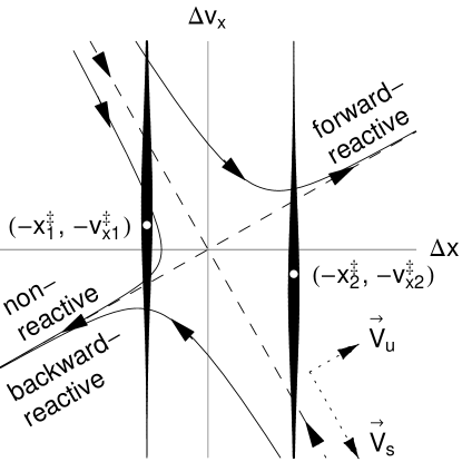
Figure 1: Phase portrait illustrating the relative dynamics in the reactive degree of freedom. Dashed lines indicate the stable and unstable manifolds of the equilibrium point, and the dotted arrows display the corresponding eigenvectors that span the diagonal coordinate system. Solid curves illustrate representative trajectories. White dots indicate two possibilities for the position and velocity of the TS trajectory at time $t=0$, the vertical lines the corresponding barrier ensembles. The probability density is given by the line widths.

For all values of $\gamma$ and $\omega_{x}$, the eigenvalue $\epsilon_{\text{u}}$ is positive, whereas $\epsilon_{\text{s}}$ is negative. They correspond to one-dimensional stable and unstable subspaces within the reactive degree of freedom which, together with representative trajectories, are illustrated in Fig. 1. The coordinate $\Delta x_{\text{u}}$ determines the fate of a trajectory in the remote future: Trajectories with $\Delta x_{\text{u}}>0$ descend into the product well, those with $\Delta x_{\text{u}}<0$ into the reactant well. Similarly, a stable coordinate $\Delta x_{\text{s}}>0$ indicates a trajectory that comes out of the product well in the distant past, whereas a trajectory with $\Delta x_{\text{s}}<0$ comes out of the reactant well. A forward-reactive trajectory that changes from reactants to products is thus characterized by $\Delta x_{\text{s}}<0$ and $\Delta x_{\text{u}}>0$, whereas a backward-reactive trajectory has $\Delta x_{\text{s}}>0$ and $\Delta x_{\text{u}}<0$. Each reactive trajectory crosses the line $\Delta x=0$ once and only once. This line, or in several degrees of freedom the hypersurface defined by this condition, can therefore serve as a recrossing-free dividing surface between reactants and products. Furthermore, the invariant stable and unstable subspaces themselves act as separatrices between reactive and nonreactive trajectories. Once the initial condition of a trajectory is known relative to these separatrices, it can unambiguously be classified as reactive or non-reactive.

III The Barrier Ensemble

The rate calculation of infrequent events —such as that in chemical reactions— can be greatly simplified by sampling trajectories in the transition state region rather than in the reactant region Keck (1962, 1967); Chandler (1978); Grimmelmann et al. (1981); Rejto and Andersen (1990). The transition path sampling technique, for example, focuses exclusively on reactive trajectories and therefore mitigates the difficulty of studying high-dimensional systems Dellago et al. (1998, 1999); Bolhuis et al. (2002); Dellago et al. (2002); MacFadyen and Andricioaei (2005). Nonetheless, the rate of infrequent events has long been known to be described by a flux-flux correlation function relative to a fixed dividing surface Yamamoto (1960); Zwanzig (1965); Chandler (1978). (But see Ref. Xing and Andricioaei, 2006 for a recent enhanced-sampling strategy to smooth the potential and thereby speed up the calculations.) One difficulty in computing the correlation function, however, is the need for the simulated trajectories to be evolved for very long times simply to determine which trajectories are reactive. We will show below that the use of the time-dependent TST dividing surface may allow one to resolve that question in a more efficient way by identifying the nature of the trajectory —viz. reactive or not— at significantly earlier evolution times.

In order to sample the reactive trajectories efficiently, it is useful to use initial conditions in which all the particles are placed on the fixed TST dividing surface ($x=0$) at $t=0$. That choice guarantees that the trajectories will cross the surface at least once, but it does not prevent them from recrossing it. Consistent with the Boltzmann weighting in the flux-flux-correlation function Yamamoto (1960); Zwanzig (1965); Chandler (1978), the initial conditions are distributed along the stable transverse direction $y$ and the velocities according to the probability density function,

$$f(x,y,v_{x},v_{y})=(2\pi\,k_{\text{B}}T)^{3/2}\,\omega_{y}\,\times\\ \exp\left\{-(\omega_{y}^{2}y^{2}+v_{x}^{2}+v_{y}^{2})/2\,k_{\text{B}}T\right\}\,\delta(x)\;.$$ (18)

This choice defines the barrier ensemble. The integration of the Boltzmann-weighted flux of these states gives the TST estimate of the numerator of the rate expression. If all these states were reactive and never recrossed (returned to) the fixed TST dividing surface, this estimate would be exact. The questions to be resolved below concern the deviation of the true dynamics from this TST estimate. These question will be investigated for both harmonic and anharmonic barriers. In all cases, the initial conditions will be sampled from the same barrier ensemble (18).

A stochastic trajectory is determined not only by its initial condition, but also by the specific instance of the fluctuating force that is acting upon it. In a full-fledged rate calculation, for example, an average has to be taken over both the initial conditions and the noise. The focus of this paper, however, is the information that can be obtained about the microscopic reaction dynamics using the moving TS surface. For simplicitly, a particular instance of the noise has therefore been used to illustrate most of the results. Nevertheless, the calculations presented here were repeated for several such noise sequences always leading to the same qualitative conclusions and thereby confirming that the results shown here are indeed typical. (These are not shown here for the sake of brevity.) While averages over the noise will tend to wipe out much of this microscopic detail, it is instructive to confirm the convergence of the identification of trajectories in calculating averages. In what follows, the average of the forward and backward reaction probability will be used to illustrate the convergence and degree of accuracy achievable using the moving TS surface to identify the reactive trajectories.

IV Analytic results

Although anharmonicities have to be addessed in a typical chemical system, it is helpful to begin with the harmonic limiting case because it is amenable to an analytic treatment. On the one hand, the harmonic limit illustrates the level of microscopic detail in which the moving TST method allows one to describe the reaction mechanism. On the other hand, the analytic results derived here provide a benchmark against which the performance of the numerical calculations of Sec. V can be assessed.

IV.1 Reaction probabilities

The fate of individual trajectories in the barrier ensemble (18) can easily be determined if their initial conditions are transformed into relative coordinates. The projection onto the reactive degree of freedom is illustrated in Fig. 1. Since in space-fixed coordinates the barrier ensemble is centered around $\vec{q}=\vec{v}=0$, the distribution function in relative coordinates is peaked at the stochastic position $\Delta\vec{q}=-\vec{q}_{\alpha}^{\ddagger}(0)$, $\Delta\vec{v}=-\vec{v}_{\alpha}^{\ddagger}(0)$. It reads explicitly

$$f_{\text{rel}}(\Delta x,\Delta y,\Delta v_{x},\Delta v_{y})=(2\pi\,k_{\text{B}}T)^{3/2}\,\omega_{y}\,\times\\ \exp\left\{-(\omega_{y}^{2}(\Delta y+y_{\alpha}^{\ddagger})^{2}+(\Delta v_{x}+v_{x\alpha}^{\ddagger})^{2}+(\Delta v_{y}+v_{y\alpha}^{\ddagger})^{2})/2\,k_{\text{B}}T\right\}\,\delta(\Delta x+x_{\alpha}^{\ddagger})\;.$$ (19)

The forward-reactive part of the ensemble is formed by those trajectories whose initial velocity $\Delta v_{x}$ is so large that the trajectory lies above both the stable and the unstable manifold of the equilibrium point. The knowledge of the eigenvectors (II.3) allows one to locate these separatrices quantitatively. Reactive trajectories are thus found to be characterized by the condition

$$\Delta v_{x}>\Delta v_{x,\text{min}}:=\begin{cases}-x_{\alpha}^{\ddagger}\epsilon_{\text{s}}&:\quad x_{\alpha}^{\ddagger}>0\;,\\ -x_{\alpha}^{\ddagger}\epsilon_{\text{u}}&:\quad x_{\alpha}^{\ddagger}<0\;.\end{cases}$$ (20)

Therefore, the probability for a member of the barrier ensemble to be forward-reactive is given by

$$P_{\text{f}} =\int d\Delta x\int_{\Delta v_{x}>\Delta v_{x,\text{min}}}d\Delta v_{x}\,\times$$

$$\hskip 50.00008pt\int d\Delta y\int d\Delta v_{y}\;f_{\text{rel}}(\Delta x,\Delta y,\Delta v_{x},\Delta v_{y})$$

or

$$P_{\text{f}} =(2\pi\,k_{\text{B}}T)^{-1/2}\,\times$$

$$\hskip 40.00006pt\int_{\Delta v_{x,\text{min}}}^{\infty}d\Delta v_{x}\exp\left\{-(\Delta v_{x}+v_{x\alpha}^{\ddagger})^{2}/2\,k_{\text{B}}T\right\}$$

$$=\frac{1}{2}\operatorname{erfc}\left(\frac{\Delta v_{x,\text{min}}+v_{x\alpha}^{\ddagger}}{\sqrt{2\,k_{\text{B}}T}}\right)\;,$$ (21)

which has been written in terms of the complementary error function Abramowitz and Stegun (1984)

$$\operatorname{erfc}(x)=\frac{2}{\sqrt{\pi}}\int_{x}^{\infty}\exp(-t^{2})\,dt\;.$$ (22)

In a similar manner, backward-reactive trajectories satisfy

$$\Delta v_{x}<\Delta v_{x,\text{max}}:=\begin{cases}-x_{\alpha}^{\ddagger}\epsilon_{\text{u}}&:\quad x_{\alpha}^{\ddagger}>0\;,\\ -x_{\alpha}^{\ddagger}\epsilon_{\text{s}}&:\quad x_{\alpha}^{\ddagger}<0\;,\end{cases}$$ (23)

and their probability in the ensemble is

$$P_{\text{b}}=\frac{1}{2}\operatorname{erfc}\left(-\frac{\Delta v_{x,\text{max}}+v_{x\alpha}^{\ddagger}}{\sqrt{2\,k_{\text{B}}T}}\right)\;.$$ (24)

IV.2 Reaction times

In contradistinction to a space-fixed dividing surface, the moving TS surface is crossed once and only once by each reactive trajectory. This allows us to define a unique reaction time $\Delta t^{\ddagger}$ for each reactive trajectory: It is the time when the trajectory crosses the dividing surface, relative to the initial time when the coordinates are specified by the barrier ensemble. If the initial conditions $\Delta x_{\text{u}}(0)$ and $\Delta x_{\text{s}}(0)$ in the reactive degree of freedom are prescribed, the reaction time can be calculated explicitly. The dynamics of the reactive degree of freedom is given by

$$\Delta x_{\text{u}}(t)=\Delta x_{\text{u}}(0)e^{\epsilon_{\text{u}}t}\;,\qquad\Delta x_{\text{s}}(t)=\Delta x_{\text{s}}(0)e^{\epsilon_{\text{s}}t}\;.$$ (25)

The dividing surface is characterized by the condition $\Delta x=0$, which can be rewritten in relative coordinates as $\Delta x_{\text{u}}=-\Delta x_{\text{s}}$. The reaction time $\Delta t^{\ddagger}$ at which this condition is satisfied is easily found to be

$$\Delta t^{\ddagger} =\frac{1}{\epsilon_{\text{u}}-\epsilon_{\text{s}}}\,\ln\frac{-\Delta x_{\text{s}}(0)}{\Delta x_{\text{u}}(0)}$$

$$=\frac{1}{\epsilon_{\text{u}}-\epsilon_{\text{s}}}\,\ln\frac{\Delta v_{x}(0)-\epsilon_{\text{u}}\Delta x(0)}{\Delta v_{x}(0)-\epsilon_{\text{s}}\Delta x(0)}\;.$$ (26)

It is defined for all initial conditions that are either forward- or backward-reactive. For a forward-reactive trajectory, $\Delta v_{x}(0)>0$. Because $\epsilon_{\text{u}}>0$ and $\epsilon_{\text{s}}<0$, it can easily be seen from Eq. (IV.2) that $\Delta t^{\ddagger}>0$ if $\Delta x(0)<0$, as it should be for trajectories that start on the reactant side of the dividing surface and are still to cross it. Similarly, a trajectory with $\Delta x(0)>0$ is already on the product side, and its reaction time is negative. A backward-reactive trajectory, on the other hand, has an initial velocity $\Delta v_{x}(0)<0$. In this case, $\Delta t^{\ddagger}<0$ if $\Delta x(0)<0$ and $\Delta t^{\ddagger}>0$ if $\Delta x(0)>0$.

If the initial position $\Delta x(0)$ is fixed, the reaction time (IV.2) tends to zero as $\Delta v_{x}(0)\to\infty$: Trajectories with large initial velocities cross the barrier fast. On the other hand, as the separatrices that bound the reactive region are approached, i.e. $\Delta v_{x}(0)\to\epsilon_{\text{u}}\Delta x(0)$ if $\Delta x(0)>0$ or $\Delta v_{x}(0)\to\epsilon_{\text{s}}\Delta x(0)$ if $\Delta x(0)<0$, trajectories keep barely enough energy to cross the barrier, and their reaction times tend to $+\infty$ or $-\infty$, respectively.

Once the reaction time is given as a function of initial conditions, the distribution for the forward- or backward-reactive part of the barrier ensemble (18) is readily obtained. In the former case, its probability distribution function is given by

$$p(\Delta t)=\frac{1}{P_{\text{f}}}\int d\Delta x\int_{\Delta v_{x}>\Delta v_{x,\text{min}}}d\Delta v_{x}\,\times\\ \int d\Delta y\int d\Delta v_{y}\;f_{\text{rel}}(\Delta x,\Delta y,\Delta v_{x},\Delta v_{y})\,\times\\ \delta(\Delta t-\Delta t^{\ddagger}(\Delta x,\Delta v_{x},\Delta y,\Delta v_{y}))\;.$$ (27)

The normalization factor $1/P_{\text{f}}$ accounts for the fact that only the forward-reactive part of the ensemble contributes to the distribution.

The distribution function (27) can in its most convenient form be written in terms of the dimensionless scaled time $\Delta\tau^{\ddagger}=(\epsilon_{\text{u}}-\epsilon_{\text{s}})\Delta t^{\ddagger}$. It then reads

$$\tilde{p}(\Delta\tau^{\ddagger})= \frac{1}{\epsilon_{\text{u}}-\epsilon_{\text{s}}}\,p(\Delta\tau^{\ddagger}/(\epsilon_{\text{u}}-\epsilon_{\text{s}}))$$

$$= \frac{|r|}{\sqrt{\pi}P_{\text{f}}}\,\frac{e^{\Delta\tau^{\ddagger}}}{(1-e^{\Delta\tau^{\ddagger}})^{2}}\,\times$$

$$\exp\left\{-\left(\frac{r}{1-e^{-\Delta\tau^{\ddagger}}}+w\right)^{2}\right\}\;,$$ (28)

where

$$r=\frac{q_{\alpha}^{\ddagger}(0)\,(\epsilon_{\text{u}}-\epsilon_{\text{s}})}{\sqrt{2\,k_{\text{B}}T}}\;,$$ (29)

$$w=\frac{v_{\alpha}^{\ddagger}(0)-\epsilon_{\text{u}}q_{\alpha}^{\ddagger}(0)}{\sqrt{2\,k_{\text{B}}T}}\;.$$ (30)

The reaction probability $P_{\text{f}}$ can be written in terms of $r$ and $w$ as

$$P_{\text{f}}=\begin{cases}\frac{1}{2}\operatorname{erfc}(r+w)&:\quad r>0\;,\\ \frac{1}{2}\operatorname{erfc}(w)&:\quad r<0\;.\end{cases}$$ (31)

The valid range of $\Delta\tau^{\ddagger}$ is $0<\Delta\tau^{\ddagger}<\infty$ if $q_{\alpha}^{\ddagger}(0)>0$ and $-\infty<\Delta\tau^{\ddagger}<0$ if $q_{\alpha}^{\ddagger}(0)<0$. The distribution function (IV.2) is normalized so that its integral over that range is one. Remarkably, the distribution depends only on the two parameters $r$ and $w$, even though the system dynamics and the distribution of initial conditions are determined by the five parameters $\omega_{\text{b}}$, $\gamma$, $T$, $q_{\alpha}^{\ddagger}(0)$ and $v_{\alpha}^{\ddagger}(0)$.

In a similar manner, the distribution of reaction times can be computed for the backward-reactive part of the ensemble. The result is again given by Eq. (IV.2), except that the valid range is now $-\infty<\Delta\tau^{\ddagger}<0$ if $q_{\alpha}^{\ddagger}(0)>0$ and $0<\Delta\tau^{\ddagger}<\infty$ if $q_{\alpha}^{\ddagger}(0)<0$. To obtain the proper normalization, the reaction probability $P_{\text{f}}$ in the prefactor of Eq. (IV.2) must be replaced by the backward-reaction probability $P_{\text{b}}$, which in terms of the scaled parameters reads

$$P_{\text{b}}=\begin{cases}\frac{1}{2}\operatorname{erfc}(-w)&:\quad r>0\;,\\ \frac{1}{2}\operatorname{erfc}(-r-w)&:\quad r<0\;.\end{cases}$$ (32)

Figure 2: The distribution (IV.2) of reaction times (a) for $w=1$ and $r=0.2$ (solid), $r=0.5$ (dashed) and $r=1$ (dotted), (b) for $w=-1$ and $r=-0.2$ (solid), $r=-0.5$ (dashed) and $r=-1$ (dotted).

As can be seen from Fig. 2, the reaction-time distribution (IV.2) is highly asymmetric around its peak. The probability distribution function is flat at $\tau=0$, where all of its derivatives are zero. For large $|\tau|$, it decays exponentially like

$$\tilde{p}(\Delta\tau^{\ddagger})\approx\begin{cases}\frac{r\,e^{-(r+w)^{2}}}{\sqrt{\pi}\,P_{\text{f}}}\,e^{-\Delta\tau^{\ddagger}}\\ \hskip 40.00006pt\text{if }q_{\alpha}^{\ddagger}(0)>0,\quad\Delta\tau^{\ddagger}\to+\infty\;,\\[8.61108pt] \frac{r\,e^{-w^{2}}}{\sqrt{\pi}\,P_{\text{f}}}\,e^{\Delta\tau^{\ddagger}}\\ \hskip 40.00006pt\text{if }q_{\alpha}^{\ddagger}(0)<0,\quad\Delta\tau^{\ddagger}\to-\infty\;.\end{cases}$$ (33)

Because the distribution is so highly asymmetric, the average reaction time will be significantly larger than the most probable reaction time that is indicated by the maximum of the distribution function.

V Numerical results

As soon as the anharmonicities of the potential in a realistic chemical system have to be taken into account, the equations of motion can no longer be solved analytically, and recourse must be taken to numerical methods. In what follows, the initial conditions, at $t=0$, are chosen from the distribution in Eq. (18). All trajectories are evolved forward and backward in time to $t=\pm T_{\text{int}}/2$ using the stochastic integration algorithm introduced by Ermak and Buckholz Ermak and Buckholz (1980); Allen and Tildesley (1987). For the backward propagation, the integration scheme was modified as described in the appendix. In a conventional calculation of the exact rate expresssion, reactive trajectories are identified according to the positions they attain at the start and end of the integration interval: Trajectories that at $t=-T_{\text{int}}/2$ and $t=+T_{\text{int}}/2$ are located on opposite sides of the space-fixed dividing surface $x=0$ are classified as forward- or backward-reactive; others are classified as nonreactive. This criterion, however, is only reliable if the total integration time $T_{\text{int}}$ is sufficiently large. At short times, recrossings of the dividing surface introduce unavoidable errors.

An alternative criterion for the identification of reactive trajectories is obtained if the space-fixed dividing surface is replaced by the moving TS surface described above. In the most naive implementation, trajectories can be classified as reactive if they are on opposite sides of the moving TS surface at $t=\pm T_{\text{int}}$. If the moving-TS-surface algorithm is used instead, $T_{\text{int}}$ can be reduced by as much as a factor of 2 while still obtaining nearly accurate results. In addition, given that the moving TS surface is exactly free of recrossings in the harmonic limit and approximately so in an anharmonic potential, the integration can be stopped as soon as a trajectory crosses the moving surface: There is no need to follow the trajectory further and check for recrossings. Therefore, when the moving TS surface is used, the actual integration time will on average be much smaller than the nominal integration time $T_{\text{int}}$.

The reliability of this identification is illustrated below using the two-dimensional saddle point potential of Eq. 4 with and without anharmonicity, $k$. In all of the numerical calculations, the units are chosen for simplicity such that $k_{\text{B}}T=1$. The friction is isotropic, with $\gamma=0.2$ in these units, and selected so as to be near the turnover between the energy- and space-diffusion limited regimes. Although most of the calculations assume the same fixed noise sequence, averages of the forward and backward reaction probabilities over the noise are also shown below. In the former, the number of trajectories is fixed at $N_{\rm t}=15\,000$, which is large enough to make statistical errors negligible. In the single-noise calculations on the two-dimensional harmonic barrier, the transverse frequency $\omega_{y}=1.5$, and the barrier frequency is set to $\omega_{x}=1.0$. The latter is reduced to $\omega_{x}=0.75$ for the noise-averaging and in the nonlinear cases in order to accentuate the nonlinear coupling.

V.1 Harmonic Systems

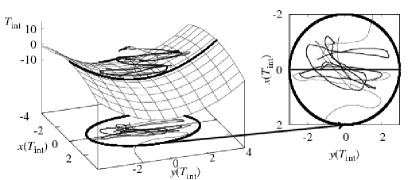
Figure 3: The evolution of a member of the ensemble and the Transition State Trajectory depicted as the gray and black lines, respectively. The underlying potential is included, and the fixed transition state $x=0$ is highlighted by the heavy black line. The time-independent projection is shown on the base of the figure. The sample trajectory is backward-reactive since it is a reactant in the future and product in the past. As can be seen, the Transition State Trajectory remains in the vicinity of the barrier for all times.

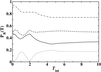
Figure 4: Reaction probabilities calculated using the fixed dividing surface displayed as a function of total integration time. The fractions of forward-reactive, backward-reactive, and nonreactive trajectories are shown as the solid, dashed, and dotted lines, respectively. The dash-dotted line represents the fraction of trajectories that cross the surface only once at $T_{\text{int}}=0$. In these simulations, $N_{\rm t}=15000$ trajectories were integrated, the friction constant $\gamma=0.2$, and the barrier frequency is $\omega_{x}=1$.

A typical reactive trajectory and the TS trajectory in the harmonic limit ($k=0$), are shown in Fig. 3. Clearly, the space-fixed dividing surface $x=0$, in contrast to the moving TS surface, is crossed many times. The respective percentages of trajectories classified either as reactive and nonreactive using the fixed dividing surface are displayed as a function of integration time in Fig. 4. Because all trajectories start on the dividing surface, at very short times, every trajectory is classified as either forward- or backward-reactive. Subsequent recrossings of the transition state result in transient fluctuations of the reaction probabilities that slowly approach the true, long-time values. Figure 4 also shows the percentage of trajectories that are nonreactive as well as those that cross the fixed dividing surface only once at $T_{\rm int}=0$. The latter comprise the majority of the reaction events, whereas the percentage contributed by reactive trajectories is comparatively small. Nevertheless, the fluctuations in the computed reaction probabilities that are caused by recrossings are considerable.

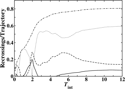
Figure 5: The number of recrossings (dot-dashed line) of the fixed transition state normalized by the total number of trajectories. The components of the total that resulted in a forward-reactive or backward-reactive trajectory are shown as the solid and dashed lines, respectively. Recrossings that resulted in a nonreactive trajectory are displayed as the dotted line. The simulation parameters are the same as in Fig. 4.

Because recrossings are crucial to the performance of the algorithm, it is instructive to analyze them in more detail. Figure 5 shows the average number of recrossings per trajectory as a function of the total integration time. The trivial crossing of the dividing surface that all trajectories undergo at $t=0$ is not included. The number increases monotonically as the trajectories cross and recross the transition state. Eventually, it reaches a plateau as they leave the barrier region and are lost into either the product or reactant states. In addition, Fig. 5 decomposes the total number of recrossings into those recrossings that occur on trajectories that are found to be forward-reactive, backward-reactive or nonreactive at the given integration time. Because the classification of a particular trajectory can change with increasing integration time, these contributions are not monotonic. Most prominently, as the number of nonreactive trajectories decreases almost to zero at $T_{\text{int}}\approx 2$ (see Fig. 4), the contribution of nonreactive trajectories shows the same behavior. For large integration times, the largest contribution to recrossings stems from nonreactive trajectories, which are bound to recross the dividing surface at least once. In fact, a comparison of Fig. 4 and Fig. 5 reveals that nonreactive trajectories on average recross more than three times before they finally leave the barrier region. Most of the reactive trajectories, by contrast, do not recross, and their contribution to the recrossing statistics is much smaller. Asymptotically, both forward and backward reactive trajectories recross on average approximately 0.25 times.

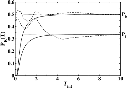
Figure 6: Reaction probabilities as a function of integration time calculated using the moving (solid curves) or the fixed (dashed curves) dividing surface. The upper set of curves represents forward-reactive probabilities, with the lower set depicting the corresponding back reactions. The dotted curves indicate the asymptotic values $P_{\text{f}}=0.3332$ and $P_{\text{b}}=0.4993$ calculated from Eq. (31) or (32), respectively. The simulation parameters are the same as in Fig. 4.

The dynamics is greatly simplified if the moving TS surface is used instead of the fixed one. Reaction probabilities computed using either surface are compared in Fig. 6. Because the trajectories start at a distance from the moving TS surface, the corresponding rates are zero for short integration times. They then steadily increase toward the true long-time probabilities. Since the dividing surface cannot be recrossed, the asymptotic values are approached monotonically. The erratic fluctuations of the computed reaction probability that the fixed surface produces are absent if the moving TS surface is used, so that a strict lower bound for the reaction probability is obtained even for very short integration times. In quantitative terms, the moving TS surface identifies a trajectory as reactive if its reaction time $\Delta t^{\ddagger}$ lies within the integration interval, so that the finite-time reaction probability for a forward reaction is given by

$$P_{\text{f}}(T_{\text{int}})=P_{\text{f}}\times\operatorname{Prob}\left\{|\Delta t^{\ddagger}|<\frac{T_{\text{int}}}{2}\right\}\;,$$ (34)

and a similar expression for the backward-reaction probability. The reaction probabilities computed from the moving TS surface are therefore determined by the distribution (IV.2) of reaction times. The convergence toward the long-time probability is described by the long-time tail (33) of the reaction-time distribution and is exponentially fast. Indeed, Fig. 6 shows that reaction probabilities computed using the moving TS surface converge much faster than those obtained from the fixed surface. Moreover, in cases such as the current problem, in which the separatrices between reactive and non-reactive trajectories are known exactly, the reaction probabilities $P_{\text{f}}$ and $P_{\text{b}}$ can be computed a priori, without having to perform any numerical simulations. The values obtained from Eqs. (31) and (32) are also indicated in Fig. 6. They agree precisely with the asymptotic probabilities obtained from the simulation. Thus, the moving TS surface can provide accelerated convergence in the rate for finite-time computations for linear problems.

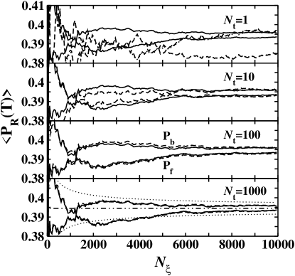
Figure 7: The reaction probabilities averaged over different instances of the noise on the harmonic potential for four different values of the number of trajectories ($N_{\rm t}$) in the ensemble. The solid lines depict the results predicted by Eqs. (31) or  (32). The dashed and dotted lines are the results obtained using the respective fixed or moving dividing surfaces. In the harmonic case, these two surfaces provide the same results and are indistinguishable. For the case of $N_{\rm t}=1000$ the light dotted lines display the $95\%$ confidence interval with respect to the number of noise sequences sampled ($N_{\xi}$). The simulation parameters are the same as those defined in Fig. 9.

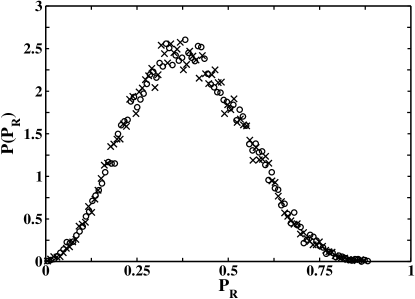
Figure 8: The distribution of reaction probabilities in the harmonic limit calculated from Eq. (31) or (32) from $N_{\xi}=20000$ different instances of the noise. The x-symbols display the results for forward-reactive probabilities and the o-symbols are for backward-reactive. The simulation parameters are the same as those defined in Fig. 9.

The analytic reaction probabilities, Eqs. (31) and (32), for the harmonic barrier represent the limiting values that are obtained for one instance of the noise using a large number $N_{\rm t}$ of trajectories. To obtain a macroscopically observable reaction probablity, one has to average these results over a large number $N_{\xi}$ of realizations of the noise. That average cannot be obtained analytically, but it can be easily calculated by a numerical quadrature. It provides a useful benchmark for the convergence of the computational schemes with respect to $N_{\rm t}$ and $N_{\xi}$. Figure 7 illustrates the forward and backward reaction probabilities, averaged over $N_{\xi}$ realizations of the noise, as a function of $N_{\xi}$ and for different values of $N_{\rm t}$. The solid and dashed curves are obtained if reactive trajectories are identified through the criteria provided by the fixed and the moving TS surfaces, respectively. As expected for a symmetric barrier, forward and backward reaction probabilities converge toward the same limit. Moreover, the distributions of forward and backward reaction probabilities agree, as shown in Fig. 8. For large $N_{\rm t}$, the results in Fig. 7 agree with the analytic value displayed as the dot-dashed curve in the figure’s bottom panel. Therein, dotted curves are used to indicate the 95% confidence interval to further illustrate that the simulations are converging toward the correct limit as expected.

The simulation results in Fig. 7 that employ the conventional criterion for identifying trajectories have been computed using the large integration time $T_{\text{int}}=21.5$, to illustrate the exact results within the error bars of the number average. However, it should be clear from Fig. 4 that the moving-TS-surface criterion often identifies reactive trajectories in less than half this time, and once so identified a trajectory does not need to be integrated further. Given that the calculation of the moving surface itself —which amounts to the calculation of the TS trajectory— takes roughly as much computational effort as the integration of an ensemble trajectory, computational savings can thus be obtained from the use of the moving surface whenever the number $N_{\rm t}$ of trajectories per noise sequence is larger than 2.

V.2 Nonlinear Systems

The true test for the usefulness of the moving transition state lies in its ability to identify reactive trajectories beyond the linear regime. If nonlinearities are present, the relative coordinate (11) does not achieve a complete separation of the relative motion from the motion of the TS Trajectory. Therefore, the moving dividing surface will not strictly be free of recrossings. However, if the nonlinearities are weak, recrossings can be expected to be rare. In these cases, the moving dividing surface will be recrossing-free to a useful approximation. Indeed, our results indicate that its advantages over a fixed dividing surface persist well beyond the harmonic limit.

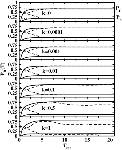
Figure 9: Reaction probabilities as a function of integration time calculated using the moving (solid line) or fixed dividing surface (dashed line) for various values of the coupling constant. The time step has been reduced to $8\times 10^{-6}$ for convergence and the barrier frequency changed to $\omega_{x}=0.75$ to accentuate the nonlinearity. For the case $k=0$, the results for the reaction probabilities as calculated from Eq. (31) or  (32) are included as the dotted lines.

We investigate the performance of the moving dividing surface in the example of the potential (4), with the coupling constant $k$ now taking non-zero values. The reaction probabilities for several different values of $k$ are displayed in Fig. 9. To accentuate the anharmonicity, the barrier frequency was reduced to $\omega_{x}=0.75$ to allow trajectories to spend more time in the barrier region before escaping. For the transverse frequency, the value $\omega_{y}=1.5$ was retained. Evidently, for sufficiently long integration times the moving transition state provides essentially the same result as the fixed dividing surface for all values of the coupling constant up to $k=0.1$. However, the reaction probabilities converge toward the long time limit monotonically and much faster than those computed with the fixed dividing surface. Therefore, the computational advantages that the moving surface offers in the harmonic limit persist even in the presence of quite substantial nonlinearities. Eventually, of course, the use of a moving dividing surface based upon the harmonic approximation ceases to be meaningful, as can be seen for $k=0.5$ and $k=1$. For the specific instance of noise used in these calculations, the results obtained from the moving and fixed dividing surfaces remain in agreement for the backward-reactive trajectories, whereas a substantial difference arises for the forward-reactive trajectories. As is to be expected of any TST scheme, in these cases the moving dividing surface overestimates the reaction probability because any trajectory that crosses the surface is assumed to be reactive, whereas the possibility of recrossings is neglected. Although not shown, a different instance of the noise does not change the trends observed in Fig. 9.

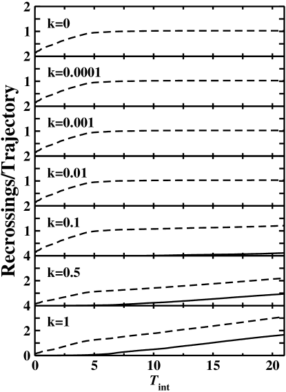
Figure 10: The average number of recrossings of the moving transition state (solid lines) and the fixed transition state (dashed line) normalized by the total number of trajectories for given values of the coupling constant. The simulation parameters are the same as those defined in Fig. 9. The values for the moving transition state are too small to be seen on the same scale in the top four panels.

As in the harmonic limit, the computational advantages of the moving dividing surface in systems with moderate nonlinearities stem from the fact that it is approximately free of recrossings. This is illustrated in Fig. 10. The average number of recrossings per trajectory of the fixed transition state exhibits similar behavior for small to moderate values of the coupling constant. It approaches approximately one recrossing per trajectory in the long-time limit. In these cases, the number of recrossings of the moving dividing surface is so much smaller than the corresponding number for the fixed surface that it is not visible in the figure. At larger coupling, the number of recrossings of the fixed dividing surface does not converge to a finite long-time limit, but instead increases linearly with the integration time. The onset of a similar behavior occurs at approximately the same value of $T_{\rm int}$ for the moving dividing surface as well.

This increase in the number of recrossings for both the fixed and the moving surfaces is caused by a small percentage of trajectories in the ensemble that never leave the TS region for negative times, but rather get trapped in an oscillation in the stable transverse degree of freedom $y$. If the value of $y$ is sufficiently large, the reactive degree of freedom $x$ in the potential (4) ceases to be unstable but instead behaves as a harmonic oscillator with a (possibly large) effective frequency $\tilde{\omega}_{x}^{2}=k\,y^{2}-\omega_{x}^{2}$. As a result of these fast oscillations in the reactive degree of freedom, the dividing surfaces are crossed many times. This mechanism has been confirmed by a detailed trajectory analysis, which for brevity we do not show. It is a rather peculiar feature of our model potential due to the presence of only one higher order coupling term in the potential (4). We would not expect such aberrant behavior to arise in a typical system.

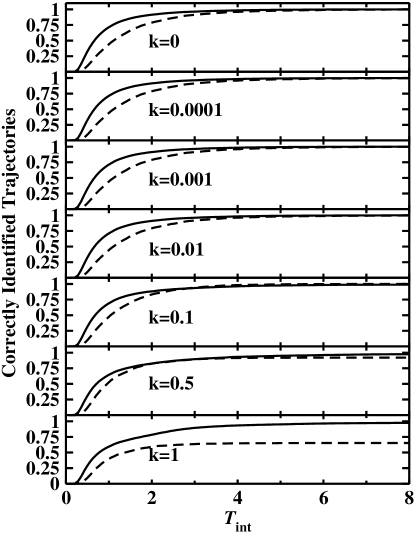
Figure 11: The fraction of correctly identified trajectories according to the moving transition state. The correct identification of a trajectory is that defined by the fixed transition state at the end of the simulation, $T_{\rm int}=21$. The correctly identified backward-reactive or forward-reactive trajectories are displayed as the solid and dashed lines, respectively. The simulation parameters are the same as those defined in Fig. 9.

It is clear from Fig. 9 that for moderately strong anharmonicities the moving transition state correctly identifies the overall number of reactive trajectories. However, that number is a macroscopic observable, and it is not immediately clear whether, on a microscopic level, individual reactive trajectories are identified correctly. The fraction of trajectories that are identified correctly by the moving transition state is displayed in Fig. 11, where the “correct” identification for a given trajectory has been assumed to be given by the fixed dividing surface for a sufficiently long integration time. In the cases of weak to moderate coupling, the classification obtained from the moving dividing surface is correct for all trajectories, but, as expected, it begins to fail for coupling strengths around $k=0.5$. The fact that the identification of the backward trajectories is poorer than that for the forward trajectories at large $k$ is not surprising. The initial distribution —particles located at the naive fixed transition state with forward velocity— disfavors backward trajectories which must recross the fixed TS at least twice more in order to reach the appropriate boundary conditions. Nevertheless, Fig. 11 confirms that the favorable behavior of the moving surface that is apparent in Fig. 9 indeed reflects a correct description of the underlying microscopic dynamics.

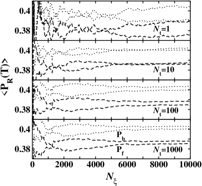
Figure 12: The reaction probabilities across an anharmonic potential (with a coupling of $k=0.1$) are shown as a smooth function of the number of different instances of the noise ($N_{\xi}$) and a discrete function of the number of trajectories ($N_{\rm t}$) used to represent the ensemble average. The dashed lines and dotted lines result from the use of the fixed or moving dividing surfaces in the identification of trajectories, respectively. Note that the ordinate ranges over the very narrow interval between .37 and .41, and hence the converged exact and approximate approaches are nearly equal. The simulation parameters are the same as those defined in Fig. 9.

Figure 12 displays the noise-averaged reaction probabilities for the fixed and moving dividing surfaces for a coupling of $k=0.1$. The results display the same convergence behavior in both cases, except that for the moving TS surface they are shifted to larger values by roughly $5\%$. This small error is due to the small percentage of trajectories that recross the moving dividing surface, as seen for a particular instance of the noise in Fig. 10. Because the potential barrier described by Eq. 4 is symmetric even for $k\neq 0$, the average values of the forward and backward reaction probabilities $P_{\rm f}$ and $P_{\rm b}$ are equal. The simulation results converge rapidly, with respect to both $N_{\rm t}$ and $N_{\xi}$, toward their limiting value. These results demonstrate that the moving TS surface retains its reliability and its computational advantages for moderate values of the anharmonicity upon noise averaging as well as for a single instance of the noise.

VI Concluding Remarks

We have recently developed an analytic method for constructing a time-dependent stochastic dividing surface that is strictly free of recrossings Bartsch et al. (2005a, b). In the present work, it has been shown that this moving dividing surface can be used to identify reactive trajectories reliably in linear and nonlinear systems: In the harmonic limit, the moving dividing surface attached to the TS trajectory is strictly free of recrossings, while in more general (nonseparable) cases it is approximately so. The identification of reactive trajectories using the moving dividing surface has been seen in this article to be fairly accurate even in the presence of large anharmonic coupling. It can be obtained in roughly half the time that is required to confirm the nature of a trajectory by numerically evolving it to its final state.

In several of the calculations presented in this article, observables have been calculated for a particular instance of the noise while averaging over the initial conditions of the subsystem. In such restricted averages, the use of the moving surface reduces the computational cost of the calculation by a factor of two or more. A typical average of an observable, however, requires one to include multiple instances of the noise. When the average is performed using the machinery of the moving TS surface, the TS trajectory must be generated for each instance of the noise. If only one system trajectory is calculated for each noise sequence, the computational effort to calculate both the sample trajectory and the moving TS surface is about the same as calculating a single (longer) trajectory. Improved CPU performance can still be obtained if one recognizes that the average should be taken by sampling several trajectories for each noise sequence. Apart from the insight into the microscopic reaction dynamics that the moving dividing surface offers, it consequently also provides computational advantages in the calculation of macroscopic observables. Moreover, the computation can be readily parallelized because the algorithm is embarrasingly parallel when sampling across the trajectories associated with a given noise sequence. (Indeed, although not discussed explicitly in the text, the codes have been parallelized across several CPUs with near linear scaling.)

In summary, we envision at least two approaches in which the TS-trajectory criterion for reactive trajectories will be useful in calculating reaction rates: (i) In harmonic (or nearly harmonic) systems, the algorithm described here provides a formally exact expression for the reaction probability given a noise sequence. This term and related averages can be used to substantially reduce the required computational time because it limits the numerical effort to a sampling of the noise. (ii) In arbitrary anharmonic systems, the criterion can be used to reduce the computational effort to calculate any correlation function —such as that in the reaction-rate expression— that relies on the correct identification of reactive trajectories. The rate expression and other related observables that can take advantage of the identification of reactive trajectories will be calculated in future work. As an illustration, the TS-trajectory criterion was seen in this work to converge the forward and backward reaction probabilities even in a fairly anharmonic case. Thus the central result of this work is: the moving dividing surface can be used reliably and efficiently to identify reactive trajectories.

Appendix: The numerical integrator

The simulations of the reaction dynamics presented in Sec. V require one to follow a stochastic trajectory numerically from $t=0$ both forward in time to $t=T/2$ and backward in time to $t=-T/2$. For the forward propagation, a standard stochastic integration scheme Ermak and Buckholz (1980); Allen and Tildesley (1987) has been implemented. The backward integration requires special care if one wishes to follow the same stochastic trajectory both forward and backward in time. The modification of the integration scheme that is necessary to this end is described here.

The forward numerical integrator for Langevin equations Ermak and Buckholz (1980); Allen and Tildesley (1987) takes the form

$$r(t+\delta t) = r(t)+c_{1}v(t)+c_{2}a(t)+\delta r\;,$$ (35)

$$v(t+\delta t) = c_{3}v(t)+c_{4}a(t)+c_{5}a(t+\delta t)+\delta v\;,$$ (36)

where $a(t)$ is the acceleration caused by the potential of mean force, the $c_{i}$ are numerical coefficients that depend on the time step $\delta t$ and the damping constant $\gamma$, and the random variables $\delta r$ and $\delta v$ are sampled from a known Gaussian distribution. Time reversal in this algorithm can be obtained through a shift in time by $-\delta t$ so that $t$ becomes $t-\delta t$ and $t+\delta t$ becomes $t$. This replacement and a simple reorganization leads to

$$r(t-\delta t) = r(t)-c_{1}v(t-\delta t)-c_{2}a(t-\delta t)-\delta r\;,$$ (37)

$$v(t-\delta t) = \frac{1}{c_{3}}\left[v(t)-c_{4}a(t-\delta t)-c_{5}a(t)-\delta v\right]\;.$$ (38)

The backward step (37) cannot be evaluated as it stands because the acceleration $a(t-\delta t)$ depends on the position $r(t-\delta t)$ that is yet to be determined. To circumvent this problem, we substitute Eq. (38) into Eq. (37) to obtain

$$r(t-\delta t)=r(t)-\frac{c_{1}}{c_{3}}\left[v(t)-c_{5}a(t)-\delta v\right]\\ -\delta r+\left(\frac{c_{1}c_{4}}{c_{3}}-c_{2}\right)a(t-\delta t)\;.$$ (39)

When the acceleration $a(t-\delta t)$ is expressed in terms of the position $r(t-\delta t)$ through the equation of motion, Eq. (39) becomes an implicit equation for the positions $r(t-\delta t)$ at the earlier time. For all but the simplest potentials, it cannot be solved explicitly. Specifically, for the anharmonic potential (4),

$$U(x,y)=-\frac{1}{2}\omega_{x}^{2}x^{2}+\frac{1}{2}\omega_{y}^{2}y^{2}+kx^{2}y^{2}\;,$$

it leads to the coupled equation system

$$x(t-\delta t)= X(t)+\left(\frac{c_{1}c_{4}}{c_{3}}-c_{2}\right)\times$$

$$\quad\left(\omega_{x}^{2}x(t-\delta t)-2kx(t-\delta t)y(t-\delta t)^{2}\right)\;,$$ (40)

$$y(t-\delta t)= Y(t)-\left(\frac{c_{1}c_{4}}{c_{3}}-c_{2}\right)\times$$

$$\quad\left(\omega_{y}^{2}y(t-\delta t)+2kx(t-\delta t)^{2}y(t-\delta t)\right)\;,$$ (41)

where $X(t)$ and $Y(t)$ denote the contributions of the first three terms in Eq. (39). In the harmonic limit $k=0$, the two equations uncouple and can be solved for simple explicit expressions for the position updates. For nonzero $k$, Eqs. (40) and (41) represent an implicit integration scheme. It can be converted into an explicit method by rearranging the terms into

$$x(t-\delta t) = \frac{X(t)}{1-\left(\frac{c_{1}c_{4}}{c_{3}}-c_{2}\right)\left(\omega_{x}^{2}-2ky(t-\delta t)^{2}\right)}\;,$$ (42)

$$y(t-\delta t) = \frac{Y(t)}{1+\left(\frac{c_{1}c_{4}}{c_{3}}-c_{2}\right)\left(\omega_{y}^{2}+2kx(t-\delta t)^{2}\right)}\;.$$ (43)

The denominators in Eqs. (42) and (43) are updated using Eqs. (40) and (41), but the unknown corrections involving $a(t-\delta t)$ are neglected because the coefficient $c_{1}c_{4}/c_{3}-c_{2}$ is of second order in the time step $\delta t$. This leads to

$$x(t-\delta t) \approx \frac{X(t)}{1-\left(\frac{c_{1}c_{4}}{c_{3}}-c_{2}\right)\left(\omega_{x}^{2}-2kY(t)^{2}\right)}\;,$$ (44)

$$y(t-\delta t) \approx \frac{Y(t)}{1+\left(\frac{c_{1}c_{4}}{c_{3}}-c_{2}\right)\left(\omega_{y}^{2}+2kX(t)^{2}\right)}\;.$$ (45)

Finally, we insert these approximations into the right-hand sides of Eq. (42) and (43) to obtain an explicit integration scheme backwards in time.

References

- Talkner and Hänggi (1995) P. Talkner and P. Hänggi, eds., New Trends in Kramers’ Reaction Rate Theory, vol. 11 of Understanding Chemical Reactivity (Kluwer Academic Publishers, Dordrecht, 1995).
- Miller (1998) W. H. Miller, Faraday Discuss. Chem. Soc. 110, 1 (1998).
- G.Truhlar et al. (1996) D. G.Truhlar, B. C. Garrett, and S. J. Klippenstein, J. Phys. Chem. 100, 12771 (1996).
- Jaffé et al. (2002) C. Jaffé, S. D. Ross, M. W. Lo, J. E. Marsden, D. Farrelly, and T. Uzer, Phys. Rev. Lett. 89, 11101 (2002).
- Koon et al. (2000) W. S. Koon, M. W. Lo, J. E. Marsden, and S. D. Ross, Chaos 10, 427 (2000).
- Komatsuzaki and Berry (2002) T. Komatsuzaki and R. S. Berry, Adv. Chem. Phys. 123, 79 (2002).
- (7) C. Jaffé, D. Farrelly, and T. Uzer, Phys. Rev. Lett. 84, 610 (2000); Phys. Rev. A 60, 3833 (1999).
- Eckhardt (1995) B. Eckhardt, J. Phys. A 28, 3469 (1995).
- Toller et al. (1985) M. Toller, G. Jacucci, G. DeLorenzi, and C. P. Flynn, Phys. Rev. B 32, 2082 (1985).
- Truhlar et al. (1985) D. G. Truhlar, A. D. Issacson, and B. C. Garrett (CRC, Boca Raton, FL, 1985), vol. 4, pp. 65–137.
- Hänggi et al. (1990) P. Hänggi, P. Talkner, and M. Borkovec, Rev. Mod. Phys. 62, 251 (1990), and references therein.
- Grote and Hynes (1980) R. F. Grote and J. T. Hynes, J. Chem. Phys. 73, 2715 (1980).
- Pollak et al. (1989) E. Pollak, H. Grabert, and P. Hänggi, J. Chem. Phys. 91, 4073 (1989).
- Mel’nikov and Meshkov (1986) V. I. Mel’nikov and S. V. Meshkov, J. Chem. Phys. 85, 1018 (1986).
- Truhlar and Garrett (1984) D. G. Truhlar and B. C. Garrett, Annu. Rev. Phys. Chem. 35, 159 (1984).
- Pollak (1990) E. Pollak, J. Chem. Phys. 93, 1116 (1990).
- Pollak (1992) E. Pollak, J. Chem. Phys. 96, 8877 (1992).
- Tucker and Pollak (1992) S. C. Tucker and E. Pollak, J. Stat. Phys. 66, 975 (1992).
- Tucker (1995) S. C. Tucker, in New Trends in Kramers’ Reaction Rate Theory, edited by P. Hänggi and P. Talkner (Kluwer Academic, The Netherlands, 1995), pp. 5–46.
- Straub et al. (1985) J. E. Straub, M. Borkovec, and B. J. Berne, J. Chem. Phys. 83, 3172 (1985).
- Straub et al. (1986) J. E. Straub, M. Borkovec, and B. J. Berne, J. Chem. Phys. 84, 1788 (1986).
- Straub et al. (1988) J. E. Straub, M. Borkovec, and B. J. Berne, J. Chem. Phys. 89, 4833 (1988).
- Pollak and Talkner (1995) E. Pollak and P. Talkner, Phys. Rev. E 51, 1868 (1995).
- Hynes (1985) J. T. Hynes, in Theory of Chemical Reaction Dynamics, edited by M. Baer (CRC, Boca Raton, FL, 1985), vol. 4, pp. 171–234.
- Pollak (1986) E. Pollak, J. Chem. Phys. 85, 865 (1986).
- Zwanzig (1973) R. Zwanzig, J. Stat. Phys. 9, 215 (1973).
- Caldeira and Leggett (1981) A. O. Caldeira and A. J. Leggett, Phys. Rev. Lett. 46, 211 (1981), Ann. Phys. (N. Y.) 149, 374 (1983).
- Graham (1990) R. Graham, J. Stat. Phys. 60, 675 (1990).
- Bartsch et al. (2005a) T. Bartsch, R. Hernandez, and T. Uzer, Phys. Rev. Lett. 95, 058301 (2005a).
- Bartsch et al. (2005b) T. Bartsch, T. Uzer, and R. Hernandez, J. Chem. Phys. 123, 204102 (2005b).
- Martens (2002) C. C. Martens, J. Chem. Phys. 116, 2516 (2002).
- Zwanzig (2001) R. Zwanzig, Nonequilibrium Statistical Mechanics (Oxford University Press, London, 2001).
- Hernandez (1994) R. Hernandez, J. Chem. Phys. 101, 9534 (1994).
- Keck (1962) J. C. Keck, Discuss. Faraday Soc. 33, 173 (1962).
- Keck (1967) J. C. Keck, Adv. Chem. Phys. 13, 85 (1967).
- Chandler (1978) D. Chandler, J. Chem. Phys. 68, 2959 (1978).
- Grimmelmann et al. (1981) E. K. Grimmelmann, J. C. Tully, and E. Helfand, J. Chem. Phys. 74, 5300 (1981).
- Rejto and Andersen (1990) P. A. Rejto and H. C. Andersen, J. Chem. Phys. 92, 6217 (1990).
- Dellago et al. (1998) C. Dellago, P. Bolhuis, F. S. Csajka, and D. Chandler, J. Chem. Phys. 108, 1964 (1998).
- Dellago et al. (1999) C. Dellago, P. Bolhuis, and D. Chandler, J. Chem. Phys. 110, 6617 (1999).
- Bolhuis et al. (2002) P. G. Bolhuis, D. Chandler, C. Dellago, and P. Geissler, Annu. Rev. Phys. Chem. 53, 291 (2002).
- Dellago et al. (2002) C. Dellago, P. G. Bolhuis, and P. Geissler, Adv. Chem. Phys. 123, 1 (2002).
- MacFadyen and Andricioaei (2005) J. MacFadyen and I. Andricioaei, J. Chem. Phys. 123, 074107 (2005), eprint 10.1063/1.2000242.
- Yamamoto (1960) T. Yamamoto, J. Chem. Phys. 33, 281 (1960).
- Zwanzig (1965) R. Zwanzig, Annu. Rev. Phys. Chem. 16, 67 (1965).
- Xing and Andricioaei (2006) C. Xing and I. Andricioaei, J. Chem. Phys. 123, 034110 (2006), eprint 10.1063/1.2159476.
- Abramowitz and Stegun (1984) M. Abramowitz and I. A. Stegun, Pocketbook of Mathematical Functions (Verlag Harri Deutsch, Frankfurt/Main, 1984).
- Ermak and Buckholz (1980) D. L. Ermak and H. Buckholz, J. Comput. Phys. 35, 169 (1980).
- Allen and Tildesley (1987) M. P. Allen and D. J. Tildesley, Computer Simulations of Liquids (Oxford, New York, 1987).