Surface Tension in Unitary Fermi Gases with Population Imbalance

Abstract

We study the effects of surface tension between normal and superfluid regions of a trapped Fermi gas at unitarity. We find that surface tension causes notable distortions in the shape of large aspect ratio clouds. Including these distortions in our theories resolves many of the apparent discrepancies among different experiments and between theory and experiments.

Experimentalists are now using dilute gases to controllably study the properties of strongly interacting systems of superfluid fermionic atoms biglistE ; ketterle1 ; ketterle2 ; randy . Recent experiments have examined the exotic circumstance where atoms with two different hyperfine spins [denoted up and down] are placed in a harmonic trap, but the number of spin-up atoms, $N_{\uparrow}$ is greater than the number of down-spin atoms $N_{\downarrow}$ ketterle1 ; ketterle2 ; randy . Spin relaxation is negligible in these experiments, so over the entire time of the experiment, the system is constrained to have a fixed polarization P=$(N_{\uparrow}-N_{\downarrow})/(N_{\uparrow}+N_{\downarrow})$. Understanding the structure of (s-wave) superfluidity in this polarized environment is an important endeavor with a long history fflo ; old1 ; old2 ; old3 and direct relevance to neutron stars, thin-film superconductors, and color superconductivity. In this paper we use the concept of surface tension to quantitatively explain controversial features seen in the density profiles of strongly interacting trapped polarized Fermi gases randy ; ketterle1 ; ketterle2 .

The simplest theories of trapped Fermi gases theja ; chevy ; new1 ; new2 ; ho (most relying on local density approximations [LDA] and assuming zero temperature) predict that the atomic cloud phase separates into a central superfluid region, in which the density of both spin species are equal, surrounded by a polarized normal shell shells . This basic structure was observed in two separate experiments randy ; ketterle1 ; ketterle2 , however some experimental details are at odds with these theoretical predictions. For $P>0.1$, the Rice experiments randy find a double peaked axial density difference, $n_{d}^{(a)}(z)=\int dx\,dy\,[n_{\uparrow}({\bf r})-n_{\downarrow}({\bf r})]$, where $n_{\uparrow/\downarrow}({\bf r})$ is the density of up and down spin atoms. In a previous paper theja , we argued that this structure pointed to a breakdown of the local density approximation, despite the fact that dimensional arguments suggested that the LDA should work well. Conversely, the results of the MIT experiments ketterle1 ; ketterle2 are fully consistent with a local density approximation, but show a polarization driven superfluid-normal phase transition at $P\sim 0.70$. This phase transition was not seen in the Rice experiments and is not found in most theories at unitarity theja ; chevy ; new1 ; new2 . Here we show that surface tension in the boundary between normal and superfluid regions distorts the cloud in exactly the right way to account for the unusual features seen at Rice. We also show that surface tension plays a much smaller role in the MIT experiments, where the atomic clouds are larger and more spherical, and we are thus able to account for the fact that the MIT experiment is consistent with the local density approximation. Finally, we show that for $P\gtrsim 0.7$, the Rice data shows a sudden drop in surface tension. Since such a drop would be expected if the system underwent a superfluid-normal phase transition, this observation may reconcile the apparent differences in the experiments. We currently lack a quantitative theory of the superfluid-normal phase transition at unitarity.

In this letter we consider the unitary regime, where the scattering length is infinite and the only lengthscale in the problem is the interparticle spacing. Taking a two-shell structure, with a superfluid core and a normal fluid shell, we model the free energy of a trapped gas as

$$F=\int_{S}d^{3}rf_{s}[\mu(r),h]+\int_{N}d^{3}rf_{n}[\mu(r),h]+\int_{\partial}d^{2}r\sigma[\mu(r),h],$$ (1)

where $\int_{S/N}$ represents the integral over the superfluid/normal region, $\int_{\partial}$ corresponds to an integral over the boundary, $f_{s/n}=-\int n^{(s)/(n)}d\mu$ represent the free energy density of the superfluid/normal gas and $\sigma$ represents the surface tension in the boundary. The energy densities are a function of the local chemical potentials $\mu(r)=[\mu_{\uparrow}(r)+\mu_{\downarrow}(r)]/2=\mu_{0}-V(r),$ and $h=[\mu_{\uparrow}(r)-\mu_{\downarrow}(r)]/2$, where $V(r)=b_{\perp}\rho^{2}+b_{z}z^{2}=\frac{1}{2}m\omega^{2}(\lambda^{2}\rho^{2}+z^{2})$ is the trapping potential, with $\lambda\approx 50$ for the Rice experiments and $\lambda\approx 5$ at MIT. The shape of the boundary, and the parameters $\mu_{0}$ and $h$, are determined by minimizing eq. (1) with respect to the boundary with the constraint that $N_{\uparrow/\downarrow}=\int_{S}d^{3}r\ n^{(s)}_{\uparrow/\downarrow}+\int_{N}d^{3}r\ n^{(n)}_{\uparrow/\downarrow}$. This approach is a generalization of one used by Chevy chevy , where the boundary term was absent. Universality allows us to write the free energy density as

$$f_{s,n}(r)=\biggr{(}-\frac{2}{15\pi^{2}}\biggr{)}\biggr{(}\frac{2m}{\hbar^{2}}\biggr{)}^{3/2}\zeta_{s,n}\mu_{s,n}(r)^{5/2},$$ (2)

where $\zeta_{s}=1/(1+\beta)^{3/2}$, $\zeta_{n}=1/2$, and $\beta\approx-0.545$ is a universal many-body parameter parabeta . The relevant chemical potentials are $\mu_{s}(r)=\mu(r)$ and $\mu_{n}(r)=\mu_{\uparrow}(r)\equiv\mu(r)+h$. The density of each spin component is $n_{\uparrow,\downarrow}=-\partial f/\partial\mu$. The fact that the particle spacing is the only length scale constrains the surface tension to have the form $\sigma=(\hbar^{2}/2m)n_{s}^{4/3}(r)g(\delta P/P)$, where $g$ is a function of $\delta P$, the pressure discontinuity across the domain wall, and $P$, the pressure on the superfluid side of the domain wall and $n_{s}$ is the density on the superfluid side. Introducing a universal numerical parameter $\eta$, we approximate $g$ by its value at zero pressure drop, $g(0)=\eta$, based on estimating that $\delta P/P<1.8\times 10^{-3}$  note1 .

We determine $\eta$ in two ways. First, as detailed in the appendix, a mean-field theory gradient expansion yields $\eta\approx 0.9\times 10^{-3}$. Second, we use a fitting scheme where we minimize Eq. ( 1) for a series of candidate $\eta$’s. We find that $\eta=1.0\times 10^{-3}$ matches the Rice group’s experimental data for the axial density difference at P=0.53. Given the uncontrolled nature of the mean field approximation, we believe that the similarity of the two results is purely coincidental. We use $\eta=1.0\times 10^{-3}$ for all of our predictions.

To simplify the minimization of Eq. (1) with respect to the boundary, we make the ansatz that the boundary is an ellipsoid with semi major and minor axes $\overline{\rho}$ and $\overline{z}$. Within this ansatz we analytically calculate the free energy [for brevity we omit the expressions]. We minimize this expression with respect to the parameters $\overline{\rho}$ and $\overline{z}$.

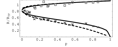
Figure 1: TOP: Comparison of the minority and majority components radii with the Rice experiments randy . Squares and crosses are the majority and minority components observed in randy , determined by looking for where the density of each component vanishes. The solid line is our theoretical prediction of the radii with zero surface tension, while the dashed line includes finite surface tension. The radii are normalized with a non-interacting Thomas-Fermi radius, $R_{TF}=\sqrt{\epsilon_{f}/b_{z})}$, where $\epsilon_{f}=\hbar\overline{\omega}(6N)^{1/3}$ with average trap frequency $\overline{\omega}=(\omega_{\perp}^{2}\omega_{z})^{1/3}$ and $N=(N_{\uparrow}+N_{\downarrow})/2.$ Note, both the normalization and the fitting procedure differ from the one used in figure 3 of randy .

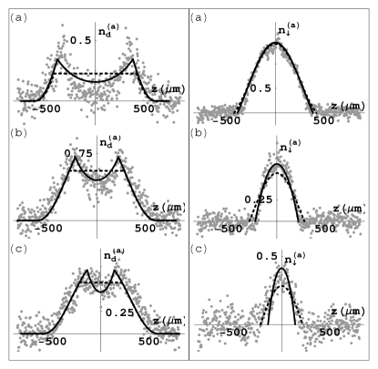
Figure 2: LEFT: Axial density difference $n_{d}^{(a)}(z)=2\pi\,\int d\rho\,\rho\,[n_{\uparrow}(z,\rho)-n_{\downarrow}(z,\rho)]$ of zero temperature harmonically trapped unitary Fermi gas in units of $[10^{6}cm^{-1}]$. Figures (a), (b), and (c) represent polarization $P=0.14$, 0.53, and 0.72 respectively. The grey points are the experimental data from reference  randy . The $P=0.14$ and $P=0.53$ data previously appeared in figure 2 of randy . The $P=0.72$ data corresponds to one of the points in figure 3 of ref randy . The dashed line is the zero surface tension density, while solid line is the finite surface tension density using $\eta=1.0\times 10^{-3}$. RIGHT: Comparison of the axial density of minority component $n_{\downarrow}^{(a)}(z)=2\pi\,\int d\rho\,\rho\,n_{\downarrow}(z,\rho)$.

To estimate the distortions, one expands Eq. (1) for small distortions: $\overline{\rho}=\rho_{0}(1+\delta_{\rho})$, and $\overline{z}=z_{0}(1+\delta_{z})$, where $\rho_{0}$ and $z_{0}$ are the lengths of the axes in the absence of surface tension. We take $\delta_{\rho}$ and $\delta_{z}$ to be order of $\delta$. Dimensional analysis gives, $\delta F/(\hbar^{2}/2m)\sim A\ \eta n^{4/3}z_{0}\rho_{0}\delta+B\ n^{5/3}z_{0}\rho_{0}^{2}\delta^{2}$, where $A$ and $B$ are constants. Assuming that $\rho_{0}$ scales with the radial Thomas-Fermi radius, the size of the distortion is then $\delta\sim 1/(\rho_{0}n^{1/3})\sim(\lambda/N)^{1/3}$.

FIG.  1 shows the calculated axial radii as a function of polarization. We compare our predictions to radii that we extract from the data used in FIG. 3 of ref. randy . We extract the radii by fitting the wings of the axial density distributions to a piecewise linear function of the form $n(z)=w\left(1-z/R\right)\theta(R-z)$, where $\theta(x)=1$ for $x>0$ and $0$ otherwise, and $w$ and $R$ are fitting parameters. This fitting procedure lets us accurately determine the edge of the cloud, while the radii extracted in randy correspond to an average radius, and are systematically larger those extracted by our method. We see that for $0.1\lesssim P\lesssim 0.7$ the experimental data is in excellent agreement with the finite surface tension theory. For $P\gtrsim 0.7$, the data used for FIG. 1 appears to be inconsistent with $\eta=1.0\times 10^{-3}$. We speculate that the deviation may be due to the superfluid-normal phase transition observed at MIT ketterle1 ; ketterle2 . We caution, however, that there are large fluctuations in the radii seen in ref. randy especially at large P. More work is needed before definitive statements can be made. The disagreement of the radii below $P_{c}\approx 0.1$ is probably attributable to finite temperature effects pcom .

In FIG.  2 and 3 we compare our predicted axial density profiles with representative data from ref. randy . As demonstrate in the left panel of FIG. 2, the finite surface tension theory captures the observed double peak structure in axial density difference for $P<0.7$. The only free parameter in this calculation is $\eta$, which as previously described we set by fitting to the $P=0.53$ data. A close examination of FIG.  2(c) reveals that the P=0.72 data is not fit quantitatively by either the finite surface tension or zero surface tension theory. As previously discussed, we suspect that the central region may not be superfluid.

As illustrated in FIG.  3, surface tension has almost no effect on the axial density of the majority component. The smallness of the effect is to be expected because the discontinuity in $n_{\uparrow}$ at the domain wall is much smaller than the discontinuity in $n_{\downarrow}$. Alternate explanations of the double-peaked axial density difference, such as anharmonicities zwierlein , would cause distortions in $n_{\uparrow}$ instead of $n_{\downarrow}$ and are not completely consistent with the experimental data replyR .

We also calculated, but do not show here, density profiles for parameters corresponding to the MIT experiments. We find that surface tension has a negligible effect on the density profile, consistent with the fact that $(\lambda/N)^{1/3}$ is 10 times smaller than at Rice.

We wish to emphasize how surprises it is to see surface tension, a phenomenon generally associated with liquid in a gas. This observation opens the possibility of other surface tension related effects in cold atoms. In particular the surface tension could have a large effect on collective modes and expansion. We speculate that surface tension should play a role in the physics of analogous systems, such as nuclear matter at high densities and quark-gluon plasmas.

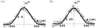
Figure 3: Comparison of the axial majority component density $n_{\uparrow}^{(a)}(z)=2\pi\,\int d\rho\,\rho\,n_{\uparrow}(z,\rho)$ in units of $[10^{6}cm^{-1}]$ with experimental data of reference randy . Figure (a) and (b) represent polarization $P=0.53$ and $P=0.72$ respectively. Symbols carry the same meanings as in Fig 2. Notice that the solid line and the dashed line coincide, indicating surface tension has no effect on the majority densities.

This work was supported by NSF grant PHY-0456261, and by the Alfred P. Sloan Foundation. We are grateful to R. Hulet and W. Li for very enlightening discussions, critical comments, and for providing us with their experimental data. We also thank M. Zwierlein for providing us with their latest results ketterle2 , and for insightful critical comments. We thank T.-L. Ho for critical comments.

APPENDIX: In this appendix we calculate the domain wall energy at the superfluid-normal interface by applying a gradient expansion to mean field theory. The domain wall energy in this approximation is given by, $E(l)=\int^{l/2}_{-l/2}dx[\gamma\mid\partial_{x}\Delta\mid^{2}+E_{bcs}(\Delta,h,\mu)-E_{n}(h,\mu)]$, where $l$, the size of the domain wall, will be determined variationally, along with $\Delta(x)$, the superfluid order parameter. The energies in the superfluid and normal phases are given by old2 ,

$$E_{bcs}(\Delta,h,\mu)=\frac{1}{2\pi^{2}}\int^{k_{+}}_{k_{-}}k^{2}dk(-h+E_{k})$$ (3)

$$+\frac{1}{2\pi^{2}}\int k^{2}dk\left[\epsilon_{k}-E_{k}+\frac{\Delta^{2}m}{\hbar^{2}k^{2}}\right]-\frac{\Delta^{2}m}{4\pi\hbar^{2}a_{s}}$$

$$E_{n}(h,\mu)=-\frac{1}{15\pi^{2}}\biggr{(}\frac{2m}{\hbar^{2}}\biggr{)}^{\frac{3}{2}}[(\mu+h)^{\frac{5}{2}}+(\mu-h)^{\frac{5}{2}}]$$ (4)

where $k_{\pm}(\vec{r})=(\pm\sqrt{h^{2}-\Delta^{2}}+\mu)^{1/2}$, $E_{k}^{2}=\epsilon_{k}^{2}+\Delta^{2}$, $\epsilon_{k}=\hbar^{2}k^{2}/2m-\mu$ and, $a_{s}$ is the s-wave scattering length.

In order to calculate the coefficient of the gradient term $\gamma$, we begin with the action $S=S_{0}+S_{int}$, where the free fermions action is $S_{0}=\sum_{\sigma}\int_{0}^{\beta}d\tau\int d^{3}\vec{r}\psi_{r\sigma}^{\dagger}[\partial_{\tau}-\mu_{\sigma}+\hbar^{2}\nabla^{2}/2m]\psi_{r\sigma}$, the interaction is $S_{int}=-U\int_{0}^{\beta}d\tau\int d^{3}\vec{r}\psi_{r\uparrow}^{\dagger}\psi_{r\downarrow}^{\dagger}\psi_{r\downarrow}\psi_{r\uparrow}$, the atomic Fermi fields are $\psi_{r\sigma}$, imaginary time is $\tau$, the inverse temperature is $\beta=1/T$ and the attractive interaction between Fermi atoms is $-U$ with $U\geq 0$. After the usual Hubbard-Stratonovich decoupling of the interaction term book and integrating out the Fermi fields, the partition function is written as $\emph{Z}=\int\emph{D}\Delta\emph{D}\Delta^{\ast}\textit{exp}[-S_{eff}(\Delta,\Delta^{\ast})]$, where $S_{eff}(\Delta,\Delta^{\ast})=\sum_{q,n}[A(q,\omega_{n})|\Delta(q)|^{2}+B(q,\omega)|\Delta(q)|^{4}+...]$ and $A(q,\omega_{n})=(1/U-T\sum_{n}\int d^{3}\vec{k}/(2\pi)^{3}G_{\uparrow}(k+q/2,\omega_{m})G_{\downarrow}(-k+q/2,\omega_{m}+\omega_{n}))$ with $G_{\sigma}(k,\omega)^{-1}=\imath\omega-\hbar^{2}k^{2}/2m+\mu_{\sigma}$. We assume that the dominant momentum dependence comes from the term which is lowest order in superfluid order parameter. We sum over Matsubara frequencies, defining $A(q)=\sum_{n}A(q,\omega_{n})$ with $\omega_{n}=(2n+1)\pi T$. In order to suppress the ultraviolet divergences in the theory, we regularize car the interaction with the s-wave scattering length by $1/U=m/4\pi\hbar^{2}a_{s}+d^{3}\vec{k}/(2\pi)^{3}m/\hbar^{2}k^{2}$. We then expand $A(q)$ to second order in q and take the zero temperature limit, finding $A(q)=m/(4\pi\hbar^{2}a_{s})-m\sqrt{\mu}/(4\pi\hbar^{2})+mq^{2}/(32\pi\hbar^{2}\sqrt{\mu})+{\cal O}(q^{4})$, which means that $\gamma=m/(32\pi\hbar^{2}\sqrt{\mu})$.

Figure 4: The value of $\eta$ as a function of $(k_{f}a_{s})^{-1}$ in zero temperature BCS approximation. At unitarity $\eta=0.0009$ is independent of the density. The Fermi wave vector $k_{f}$ is defined as $k_{f}^{3}=3\pi^{2}n_{s}$.

Taking the ansatz $\Delta(x)=(\Delta_{0}/2)[\tanh(x/l)+1]$, where $\Delta_{0}$ is the value of $\Delta$ on superfluid side of the domain wall, we numerically minimize the surface energy $E(l)$ with respect to $l$ to find the size of the domain wall $l_{m}$ and the domain wall energy. We find $l_{m}<k_{f}^{-1}$, supporting our treatment of the domain wall as very thin, but calling into question the validity of our gradient expansion. Note that we do not expand $E_{bcs}$ in powers of $\Delta$, but work with the exact expansion. Since we are considering a domain wall between a region where $\Delta=0$ and $\Delta\approx{\cal O}(E_{f})$, any expansion in $\Delta$ would require going to high order. To even capture the topology of the free energy surface, one must expand to sixth order. Thus, previous calculation of surface tension, such as Caldas’s caldas recent work, which are based on fourth order expansions are not relevant to the physics described here. By repeating this calculation at different $a_{s}$, and solving the BCS number equation and gap equation theja , we find the quantity $\eta=2mE(l_{m})/(\hbar^{2}n_{s}^{4/3})$ as a function of $a_{s}$ and $n_{s}$, where $n_{s}$ is the density on the superfluid-normal interface. In the limit of $a_{s}\rightarrow\infty$, we find $\eta=0.9\times 10^{-3}$, independent of the density and polarization. However, as seen in FIG.  4, $\eta$ has density dependence away from unitarity. As $a_{s}\rightarrow 0^{+}$, $\eta$ grows larger, hence the effects of surface tension is stronger. Therefore, in the strong BEC regime, domain walls become energetically prohibitive and the phase separated atomic system is unstable against phase coexistence old2 ; theja ; new1 . Recent theoretical work by Imambekov et al adilet studied the role of gradient terms in this deep BEC limit.

The value of $\eta$ obtained from fitting to experimental data agrees well with our mean field calculation. We believe that this agreement is coincidental as mean field theory is not expected to work well at unitarity. We also note that the experiment is performed slightly away from the resonance where the mean field approximation predicts a weak density dependance of $\eta$ note2 .

References

- (1) K. M. O’Hara et al., Science 298, 2179 (2002); M. Greiner, C. A. Regal, and D. S. Jin, Nature 426, 537 (2003); S. Jochim et al., Science 302, 2101 (2003); M. W. Zwierlein et al., Phys. Rev. Lett. 91, 250401 (2003); T. Bourdel et al., Phys. Rev. Lett. 93, 050401 (2004); C. Chin et al., Science 305, 1128 (2004); J. Kinast et al., Science 307, 1296 (2005); J. Kinast et al., Phys. Rev. Lett. 92, 150402 (2004); M. Bartenstein et al., Phys. Rev. Lett. 92, 203201 (2004); M. W. Zwierlein et al., Nature 435, 1047-1051 (2005); G. B. Partridge et al., Phys. Rev. Lett. 95, 020404 (2005).
- (2) Martin W. Zwierlein, Andr Schirotzek, Christian H. Schunck, Wolfgang Ketterle, Science, 311, 492 (2006).
- (3) Martin W. Zwierlein, Christian H. Schunck, Andr Schirotzek, and Wolfgang Ketterle, unpublished.
- (4) Guthrie B. Partridge, Wenhui Li, Ramsey I. Kamar, Yean-an Liao, and Randall G. Hulet, Science, 311, 503 (2006).
- (5) P. Fulde and R. A. Ferrell, Phys. Rev. 135, A550 (1964) and A.I. Larkin and Yu.N. Ovchinnikov, Zh. Eksp. Teor. Fiz 47, 1136 (1964) [Sov. Phys. JETP 20, 762 (1965)]; G. Sarma, J. Phys. Chem. Solids 24, 1029 (1963).
- (6) R. Combescot, Europhys. Lett. 55, 150 (2001); H. Caldas, Phys. Rev. A 69, 063602 (2004); A. Sedrakian, J. Mur-Petit, A. Polls; H. M uther, Phys. Rev. A 72, 013613 (2005); U. Lombardo, P. Nozi‘eres, P. Schuck, H.-J. Schulze, and A. Sedrakian, Phys. Rev. C 64, 064314 (2001); D.T. Son and M.A. Stephanov, Phys A 72, 013614 (2006); L. He, M. Jin and P. Zhuang, Phys B 73, 214527 (2006); P. F. Bedaque, H. Caldas, and G. Rupak, Phys. Rev. Lett. 91, 247002 (2003).
- (7) C.-H. Pao, Shin-TzaWu, and S.-K. Yip, Phys. Rev. B 73, 132506 (2006); D.E. Sheehy and L. Radzihovsky, PRL 96, 060401 (2006); W.V. Liu and F. Wilczek, Phys. Rev. Lett. 90, 047002 (2003).
- (8) J. Carlson and S. Reddy, Phys. Rev. Lett. 95, 060401 (2005); P. Castorina, M. Grasso, M. Oertel, M. Urban, and D. Zappal‘a, Phys. Rev. A 72, 025601 (2005); T. Mizushima, K. Machida, and M. Ichioka, Phys. Rev. Lett. 94, 060404 (2005).
- (9) Theja N. De Silva, Erich J. Mueller, Phys. Rev. A 73, 051602(R) (2006), preprint cond-mat/0601314.
- (10) F. Chevy, Phys. Rev. Lett. 96, 130401 (2006).
- (11) P. Pieri, and G.C. Strinati, Phys. Rev. Lett. 96, 150404 (2006); W. Yi, and L. -M. Duan, Phys. Rev. A 73, 031604(R) (2006).
- (12) J. Kinnunen, L. M. Jensen, and P. Torma, Phys. Rev. Lett. 96, 110403 (2006); M. Haque and H. T. C. Stoof, preprint, cond-mat/0601321; Zheng-Cheng Gu, Geoff Warner and Fei Zhou, preprint cond-mat/0603091; M. Iskin and C. A. R. Sa de Melo, preprint cond-mat/0604184; T. Paananen, J.-P. Martikainen, P. Torma, Phys. Rev. A 73, 053606 (2006); C.-H. Pao, S.-K. Yip, J. Phys. Condens. Matter 18, 5567 (2006); W. Yi, L.-M. Duan, Phys. Rev. A 74, 013610 (2006); M. Mannarelli, G. Nardulli, and M. Ruggieri, preprint, cond-mat/0604579.
- (13) Tin-Lun Ho and Hui Zhai, preprint cond-mat/0602568.
- (14) The superfluid and normal regions may be further subdivided, depending on interaction parameters. See theja .
- (15) J. Carlson, S.-Y. Chang, V. R. Pandharipande, and K. E. Schmidt, Phys. Rev. Lett. 91, 050401 (2003).
- (16) Laplace’s law gives, , where is the radius of curvature of the domain wall. Typical values from randy are (m)-4, m, and (m)-5.
- (17) R. Hulet, Private communications.
- (18) M. Zwierlein and W. Ketterle, preprint cond-mat/0603489.
- (19) Guthrie B. Partridge, Wenhui Li, Ramsey I. Kamar, Yean-An Liao, Randall G. Hulet, preprint cond-mat/0605581.
- (20) For example see, Functional Integrals and Collective Excitations by V. N Popov, Cambridge University Press, 1987.
- (21) C. A. R. Sa de Melo, M. Randeria, and J. R. Engelbrecht, Phys. Rev. Lett. 71, 3202 (1993).
- (22) H. Caldas, preprint cond-mat/0601148.
- (23) A. Imambekov, C. J. Bolech, M. Lukin, and E. Demler, preprint cond-mat/0604423.
- (24) The Rice experiment has a characteristic density corresponding to .