Most probable transition path in an overdamped system for a finite transition time

Abstract

The most probable transition path in a one-dimensional overdamped system is rigorously proved to possess less than two turning points. The proof is valid for any potentials, transition times, initial and final transition points.

I 1. Introduction

The overdamped stochastic equation is commonly defined as FPE

$$\frac{{\rm d}x}{{\rm d}t}=-\frac{{\rm d}U(x)}{{\rm d}x}+f(t),$$ (1)

$$\langle f(t)\rangle=0,\quad\langle f(t)f(0)\rangle=2D\delta(t).$$

The beginning of theoretical studies of such a stochastic process dates back to the celebrated works by Einstein einstein studying the Brownian motion of a free particle, which may formally be considered as an overdamped stochastic motion in a parabolic potential where the role of the generalized coordinate is played by the velocity. A more general study of overdamped stochastic processes was started by Smoluchowski smoluchowski who formulated the equation of motion for the probability density in an arbitrary overdamped system: this equation bears his name nowadays. The next milestone was the work by Kramers kramers who, in particular, formulated the problem of the noise-induced escape of an overdamped system from a metastable potential well and derived its quasi-stationary solution: the quasi-stationary escape flux was found in kramers using a stationary solution of the Smoluchowski equation:

$$J_{qs}=A_{qs}{\rm e}^{-\frac{\Delta U}{D}},\quad\quad D\ll\Delta U,$$ (2)

where $\Delta U$ is the potential barrier (assumed to be much less than the noise intensity $D$) and $A_{qs}$ is certain prefactor which depends on $D$ weakly in comparison with the exponential (activation) factor.

As follows from kramers , the escape flux becomes quasi-stationary when time greatly exceeds a characteristic value $t_{qe}\sim t_{r}\ln(\Delta U/D)$ where $t_{r}$ is a characteristic relaxation time. There were only a few theoretical works on the escape in overdamped systems on time scales $t\lesssim t_{qe}$. One of the most general of such works was the work by Shneidman schneidman who solved the non-stationary Smoluchowski equation for an arbitrary potential using the method of the Laplace integral transformation while assuming that the quasi-equilibrium in the vicinity of the bottom of the well has been formed. The latter assumption is valid only for times significantly exceeding the relaxation time $t_{r}$ while, for shorter times, results of schneidman are invalid.

The time scale $t\lesssim t_{r}$ was covered in the work our by means of the path-integral method feinman ; gy1960 ; alan1 ; lrh1 sometimes called also the method of optimal fluctuation lmd1998 . As a by-product, it was proved in our that the most probable escape path, i.e. the path providing the absolute minimum of action in the functional space $[x(\tau)]$, is monotonous i.e. $[x(\tau)]$ does not possess turning points.

In parallel to the development of the escape problem on short times, there was an interesting discussion in the 90th vugmeister ; mannella ; vugmeister1 on the transition problem on short times. This problem may be of interest in the context of the prehistory probability density prehistory and of some biological problems nigel ; lindner . Unlike the case of the escape, both the initial and final points of the transition differ from the stationary points of the noise-free system and, if they lie on one and the same slope of the potential, the transition may possess features distinctly different from those of the escape. Thus, basing on the method of optimal fluctuation feinman ; lmd1998 , the authors of vugmeister suggested that, for the short-time transition uphill the slope of the potential barrier, the most probable transition path (MPTP) may first relax close to the bottom of the well and only then go to the final point. They supported their suggestion by analytic calculations for the parabolic approximation of the potential and, seemingly, by the numerical calculations for the exact potential. However it was shown in mannella (also by means of numerical calculations within the optimal fluctuation method) that the path which first climbes up close to the barrier top and only then relaxes to the final point may provide an exponentially larger activation factor. Thus, just the latter path pretends to be the MPTP in such a case.

The further development of this problem was done in our : it demonstrated that the extreme paths, i.e. paths providing local minima of action, can possess many turning points; our provides the method how to explicitly calculate all possible (for a given transition time) extreme paths and demonstrates that, as the transition time increases, the MPTP may switch its topology from the monotonous path to the path possessing one turning point, either continuously or jump-wise.

The present work proves the general theorem stating that the extreme paths possessing more than one turning point cannot provide the absolute minimum of action i.e. the MPTP can be only either monotonous or possessing just one turning point.

It should be noted also that, apart from being necessary for a calculation of the activation energy, the MPTP may be of interest on its own: e.g. in the problem of the optimal control, the MPTP determines the dynamics of the external force which optimally enhances or suppresses a given fluctuational transition sd ; vr .

II 2. Basic equations

In this section, I briefly reproduce basic equations of the method of optimal fluctuation feinman ; lmd1998 and those of results our which will be used in the next section for the proof of the theorem.

Within the method of optimal fluctuation, the flux is sought in the form

$$J(t)=P(D,t){\rm e}^{-\frac{S_{a}(t)}{D}},\quad\quad D\ll S_{a},$$ (3)

where the prefactor is assumed to depend on $D$ much more weakly than the activation (exponential) factor while the activation energy $S_{a}$ is a minimum of the functional $S$, called action,

$$S_{a}=\min_{[x(\tau)]}S,\quad\quad S\equiv S[x(\tau)]=\int_{0}^{t}d\tau\;L,$$ (4)

$$L=\frac{1}{4}\left(\dot{x}+\frac{dU}{dx}\right)^{2},\quad\quad x(0)=x_{0},\quad\quad x(t)=x_{f}.$$

The necessary condition for a minimum of the functional is the equality of the variation $\Delta S$ to zero. The latter is equivalent to the Euler equation (EE):

$$\frac{\partial{L}}{\partial{x}}-\frac{{\rm d}}{{\rm d}t}\left(\frac{\partial{L}}{\partial{\dot{x}}}\right)=0,$$ (5)

which, for a Lagrangian of the form (4), reads as

$$\ddot{x}+\frac{{\rm d}\tilde{U}}{{\rm d}x}=0,\quad\quad\tilde{U}=-\frac{1}{2}\left(\frac{{\rm d}U}{{\rm d}x}\right)^{2}.$$ (6)

So, solutions of the EE, called extremal paths, are trajectories of the auxiliary mechanical system (6).

The quasi-energy

$$E\equiv-\partial S/\partial t=\dot{x}(\partial L/\partial\dot{x})-L=\frac{\dot{x}^{2}-(dU/dx)^{2}}{4}$$ (7)

is conserved along a solution of the EE, so that one easily derives from (7):

$$\dot{x}=\pm\sqrt{4E+(dU/dx)^{2}}.$$ (8)

It also follows from (7) that the range of allowed quasi-energies is:

$$E\geq E_{min}\equiv-\min_{[x_{0},x_{f}]}[\left(dU/dx\right)^{2}/4].$$ (9)

Eq. (8) can be integrated in quadratures. Action $S$ can be expressed in quadratures too.

For the case of escape, i.e. when the initial point is the bottom of the well ($x_{0}=x_{w}$) stable_state , $E_{min}=0$ and therefore the motion in $\tilde{U}(x)$ with a quasi-energy $E\geq E_{min}$ cannot possess turning points. Thus, the most probable escape path $[x(\tau)]$ is necessarily monotonous. On the contrary, in case of transition within one slope of the potential i.e. when both $x_{0}$ and $x_{f}$ lie between the bottom of the well $x_{w}$ and the top of the barrier $x_{b}$, the minimum quasi-energy $E_{min}$ is negative and hence a trajectory of motion in the auxiliary potential $\tilde{U}(x)$ may possess a negative quasi-energy $E<0$. In the latter case, the trajectory possesses turning points in $x_{+}$ and $x_{-}$, which are the roots of the equation

$$E=-\left(dU/dx\right)^{2}/4$$ (10)

where $x_{+/-}$ is the root nearest to $x_{f/0}$ among the roots located at the same side of $x_{0/f}$ as $x_{f/0}$:

$$(x_{+/-}-x_{f/0})(x_{f/0}-x_{0/f})\geq 0.$$ (11)

An extremal path for a given $E<0$ may turn in $x_{-}$ and $x_{+}$ any number of times. Let us classify extremal paths by their topology, namely by the overall number $N$ of turns of $[x(\tau)]$ (i.e. the number of changes of the sign of the velocity) and by the sign of the initial velocity multiplied by the sign of $x_{f}-x_{0}$: we shall use labels like “$N=3,+$” (in the case of $N=0$, the ${\rm sign}[\dot{x}(x_{f}-x_{0})]$ is necessarily “$+$”, so we shall omit the sign in the label in this case). For each topology defined as above, the extremal path is uniquely defined and, moreover, it can be implicitly expressed by means of quadratures our . The full time along an extremal of a given topology can be explicitly expressed via quadratures. To present these expressions in a compact form, it is convenient to introduce three auxiliary “times”:

$$t_{0}\equiv t_{0}(E)=t_{x_{0}\leftrightarrow x_{f}},\quad\quad$$

$$t_{+}\equiv t_{+}(E)=t_{x_{f}\leftrightarrow x_{+}},\quad\quad$$

$$t_{-}\equiv t_{-}(E)=t_{x_{-}\leftrightarrow x_{0}},$$

$$t_{a\leftrightarrow b}\equiv\left|\int_{a}^{b}\frac{dq}{\dot{q}(E,q)}\right|={\rm sign}\left[\frac{b-a}{x_{f}-x_{0}}\right]\int_{a}^{b}dq\;z(q,E),$$

$$z(q,E)\equiv{\rm sign}[x_{f}-x_{0}]\frac{1}{\sqrt{4E+(dU(q)/dq)^{2}}}.$$ (12)

For different topologies, the dependence of the full time along the extremal path on quasi-energy reads as:

$$t_{N=0}(E)=t_{0},$$ (13)

$$t_{N=2n+1,+/-}(E)=t_{0}+2t_{+/-}+(N-1)(t_{0}+t_{+}+t_{-}),$$

$$t_{N=2n+2,+/-}(E)=\pm t_{0}+N(t_{0}+t_{+}+t_{-}),$$

$$n=0,1,2,...$$

Figs. 1(c) and 2(c) show branches in the given ranges of $t$ and $E$, calculated by (13), for two characteristic cases related to Figs. 1(a,b) and 2(a,b) respectively: when $-\tilde{U}(x)$ does not possess a local minimum in between $x_{w}$ and $x_{b}$ (Fig. 1) and when it does (Fig. 2).

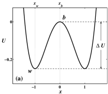
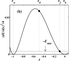
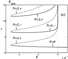
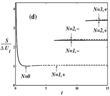
Figure 1: (a)The Duffing potential $U(x)=-x^{2}/2+x^{4}/4$; the left well and the barrier are marked by the labels w and b respectively (the cordinate $x_{w}$ of the bottom of the well and the coordinate $x_{b}$ of the top of the barrier are indicated by the dotted lines); the potential barrier $\Delta U$ is indicated by the dashed lines. (b) The function $(dU(x)/dx)^{2}/4\equiv-\tilde{U}(x)/2$ (thick solid line); the dots show the points on the curve which correspond to the initial and final points of the transition ($x_{0}=-0.5$ and $x_{f}=-0.1$ respectively); $-E_{min}$ (9) is indicated by the dashed line. (c) Different branches of $t(E)$, calculated by Eq. (13) and corresponding to different topologies of the extremal path, are shown by thick solid/dashed lines with the labels indicating the number of turning points and the sign of the initial velocity $\dot{x}(0)$ multiplied by the sign of $x_{f}-x_{0}$. (d) Different branches of the action $S(t)$ (normalized by $\Delta U_{1}\equiv U(x_{f})-U(x_{0})=0.1044$), calculated by Eq. (15), are marked similarly to the corresponding branches of $t(E)$ in (c).

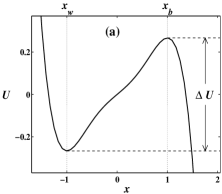
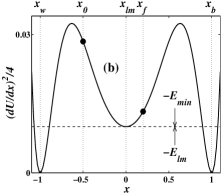
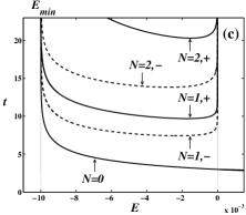
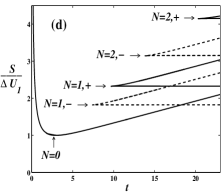
Figure 2: (a) The potential $U(x)=-x^{5}/5+0.8x^{3}/3+0.2x$; and (b) the corresponding function $(dU(x)/dx)^{2}/4\equiv-\tilde{U}(x)/2$ (dots indicate points on the curve for $x_{0}=-0.5$ and $x_{f}=0.2$); $E_{min}$ coincides with the singularity energy $E_{lm}$ related to the local minimum of $(dU(x)/dx)^{2}/4$. Figures (c) and (d) are analogous to Figs. 1(c) and 1(d) respectively. The normalization in (d) is: $\Delta U_{1}\equiv U(x_{f})-U(x_{0})\approx 0.16915$.

In order to present the results for action in a compact form, it is convenient to introduce the auxiliary actions:

$$S_{0}\equiv S_{0}(E)=\int_{x_{0}}^{x_{f}}dq\;\eta(q,E),$$ (14)

$$S_{1}\equiv S_{1}(E)=\int_{x_{0}}^{x_{f}}dq\;(\eta(q,E)-\frac{1}{2}dU/dq)$$

$$=S_{0}-\frac{1}{2}\Delta U_{1},\quad\quad\Delta U_{1}\equiv U(x_{f})-U(x_{0}),$$

$$S_{+}\equiv S_{+}(E)=\int_{x_{f}}^{x_{+}}dq\;(\eta(q,E)-\frac{1}{2}dU/dq),$$

$$S_{-}\equiv S_{-}(E)=\int_{x_{-}}^{x_{0}}dq\;(\eta(q,E)-\frac{1}{2}dU/dq),$$

$$\eta(q,E)=\frac{1}{2}\left(\frac{{\rm sign}[x_{f}-x_{0}](2E+(dU/dq)^{2})}{\sqrt{4E+(dU(q)/dq)^{2}}}+\frac{dU}{dq}\right).$$

Then $S(t)$ for various branches can be shown to be as follows our :

$$S_{N=0}(t)=S_{0},$$ (15)

$$S_{N=2n+1,+/-}(t)=S_{0}+2S_{+/-}+(N-1)(S_{1}+S_{+}+S_{-}),$$

$$S_{N=2n+2,+/-}(t)=S_{0}+(\pm 1-1)S_{1}+N(S_{1}+S_{+}+S_{-}),$$

$$n=0,1,2,...,$$

where $E\equiv E(t)$ in $S_{0},S_{1},S_{+},S_{-}$ should be taken, for a given branch $S_{N,+/-}(t)$, as a solution of the equation

$$t=t_{N,+/-}(E),$$ (16)

where the functions $t_{N,+/-}(E)$ are defined in (13) footnote3 .

Eqs. (12)-(16) describe in quadratures all possible extremals and actions along them, in the general case.

III 3. Maximum number of turning points in the MPTP

For Figs. 1 and 2, the activation energy $S_{a}(t)$ (i.e. the minimal action) appears to be constituted only by branches with “$N\leq 1$” at any $t$. For the case like in Fig. 1, such a result is intuitively predictible. But for the case like in Fig. 2, it is not so. Consider e.g. the case when $x_{0}$ and $x_{f}$ are situated in a relatively flat part of a potential while the potential beyond it is much steeper (Fig. 3(a)). Intuition might suggest that, if the transition time is large, then multiple passages within the flat part of the potential might lead to a smaller action than that for a path of the same duration but with only one turning point: the latter path might seem to necessarily involve one of the steep parts of the potential, with a very large variation of the potential, which would lead in turn to a very large action. So, the question arises whether it is a general property for the number of turning points in the MPTP to be less than 2. We prove below the theorem stating that it is. As for the intuitive argument discussed above in relation to Fig. 3, it does not contradict this theorem. Indeed, the MPTP does possess less than two turning points while it still remains within the flat part of the potential: it stays a main part of the given time in the minima of $(dU/dx)^{2}$.

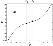
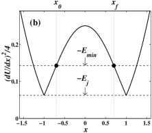
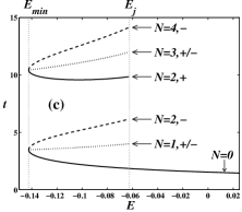
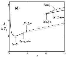
Figure 3: (a) The monotonously increasing potential $U(x)$ with the following derivative: $dU/dx=1-0.5x^{2}$ at $x\in[-1,1]$ while $dU(x)/dx=0.5\mp(x\pm 1)$ at $\mp x\in[1,\infty]$; the initial and final transition points are indicated by dots and and dotted lines: $x_{f}=-x_{0}=0.7$. (b) The function $({\rm d}U(x)/{\rm d}x)^{2}/4$ (thick solid line); the level where ${\rm d}^{2}U/{\rm d}x^{2}$ undergoes the jump is indicated by a dashed line and the label $-E_{j}$. In (c) and (d), the branches “$N=0$” and “$N=2n,+$” with $n=1,2,3,...$ are shown by the thick solid lines while branches “$N=2n,-$” and “$N=2n+1,+/-$” are shown by dashed and dotted lines respectively. In (c), $\Delta U_{1}\equiv U(x_{f})-U(x_{0})\approx 1.285667$. In (d), $S(t)$ is calculated numerically by Eq. (15) in those ranges of $t$ where the continuous paths exist while $S(t)$ is given in other ranges of $t$ by Eq. (24) with $E=E_{j}$.

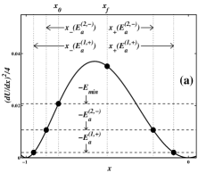
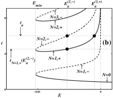
Figure 4: This figure illustrates the proof of the relation $S_{N=2,-}(t)>S_{N=1,+}(t)$ at any $t\neq t_{N=2,-}(E_{min})\equiv t_{N=1,+}(E_{min})$. For the sake of concreteness, we exploit the example of the Duffing potential as in Fig. 1 while $x_{0}=-0.8$ and $x_{f}=-0.5$. The relevant points are marked by the large dots as well as indicated by thin dotted/dashed lines and by corresponding labels.

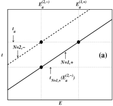
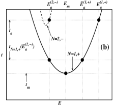
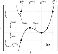
Figure 5: This figure shows schematically three characteristic cases when the function $t_{N=1,+}(E)$ in the relevant range of energies is (a) monotonous; (b) non-monotonous while there is no local maxima, (c) non-monotonous while there is a local maximum. The relevant points on the branches “$N=2,-$” and “$N=1,+$” are marked by the large dots as well as indicated by thin dotted lines and by corresponding labels.

Theorem: the activation energy $S_{a}(t)$ is constituted by the branches of action (15) with $N\leq 1$.

Proof.

1. Consider first the most common case, when $dU(x)/dx$ is continuous while $d^{2}U/dx^{2}$ is either continuous or, if it does change jump-wise, is possessing one and the same sign at both sides of the jump.

For the sake of brevity, we assume below that $(dU(x_{0})/dx_{0})^{2}\leq(dU(x_{f})/dx_{f})^{2}$. The case when the latter inequality does not hold can be proved analogously.

We use as an illustration the case shown in Fig. 4(a). Let us prove that

$$S_{N=2,-}(t)>S_{N=1,+}(t),$$ (17)

$$t\neq t_{N=2,-}(E_{min})\equiv t_{N=1,+}(E_{min})$$

(at $t=t_{N=2,-}(E_{min})\equiv t_{N=1,+}(E_{min})$, the branches “$N=2,-$” and “$N=1,+$” merge, so that the actions obviously coincide at this instant footnote_new ). Consider any time $t_{a}$ arbitrarily chosen from the range where the equation

$$t_{a}=t_{N=2,-}(E)$$ (18)

possesses at least one root footnote4 (note that if the roots do exist they are necessarily negative). Consider any of the roots of Eq. (18), $E_{a}^{(2,-)}$ (see Fig. 4(b)). As follows from Eq. (13), the time $t_{a}$ can be presented in the following form:

$$t_{a}\equiv t_{N=2,-}(E_{a}^{(2,-)})=$$ (19)

$$\quad\quad t_{0}(E_{a}^{(2,-)})+2(t_{+}(E_{a}^{(2,-)})+t_{-}(E_{a}^{(2,-)})),$$

where $t_{0},t_{+},t_{-}$ are given in Eq. (12). As follows from Eq. (15), the corresponding action can be presented as:

$$S_{N=2,-}(E_{a}^{(2,-)})=$$ (20)

$$S_{0}(E_{a}^{(2,-)})+2(S_{+}(E_{a}^{(2,-)})+S_{-}(E_{a}^{(2,-)})),$$

where $S_{0},S_{+},S_{-}$ are given in Eq. (14).

Let us turn now to the branch “$N=1,+$”. As follows from (15),

$$S_{N=1,+}(E_{a}^{(2,-)})=S_{0}(E_{a}^{(2,-)})+2S_{+}(E_{a}^{(2,-)}).$$ (21)

Comparing (20) and (21), we may present $S_{N=2,-}(t_{a})$ as

$$S_{N=2,-}(t_{a})\equiv S_{N=2,-}(E_{a}^{(2,-)})=S_{N=1,+}(E_{a}^{(2,-)})+$$

$$\quad\quad\quad\quad\quad\quad\quad\quad\quad\quad\quad\quad\quad\quad\Delta S_{2,-}\quad,$$

$$\Delta S_{2,-}\equiv 2S_{-}(E_{a}^{(2,-)}).$$ (22)

Let us consider now the equation

$$t_{a}=t_{N=1,+}(E).$$ (23)

This equation necessarily possesses at least one (negative) root which is larger than $E_{a}^{(2,-)}$. The latter is a consequence of two properties: (i) $t_{N=1,+}(E)<t_{N=2,-}(E)$ since, at a given energy, the path “$N=1,+$” is a part of the path “$N=2,-$”; (ii) $t_{N=1,+}(E)$ continuously increases to $\infty$ as $E\rightarrow-0$ and as $E\rightarrow E_{lm}-0$ (the latter is relevant only to the case with a local minimum of $(dU(x)/dx)^{2}$) footnote5 . Fig. 5 illustrates this important property of an existence of a root of Eq. (23) exceeding $E_{a}^{(2,-)}$.

Let us consider separately three characteristic cases shown in Fig. 5. In all other cases, the proof can be reduced to the combination of those for these three cases. Consider first the case when $t_{N=1,+}(E)$ is monotonously increasing in the range $[E_{a}^{(2,-)},E_{a}^{(1,+)}]$ where $E_{a}^{(1,+)}$ is such a root of Eq. (23) which exceeds $E_{a}^{(2,-)}$ while being closer to $E_{a}^{(2,-)}$ than any other root of Eq. (23) exceeding $E_{a}^{(2,-)}$ (see Fig. 5(a) or Fig. 4(b)). Using the property

$$\frac{dS_{N,+/-}}{dt}=-E,$$ (24)

where $E\equiv E(t)$ is a solution of Eq. (16) 24 , one may present $S_{N=1,+}(t_{a})$ as

$$S_{N=1,+}(t_{a})\equiv S_{N=1,+}(E_{a}^{(1,+)})=S_{N=1,+}(E_{a}^{(2,-)})+$$

$$\quad\quad\quad\quad\quad\quad\quad\quad\quad\quad\quad\quad\quad\quad\Delta S_{1,+}\quad,$$

$$\Delta S_{1,+}\equiv\int_{t_{N=1,+}(E_{a}^{(2,-)})}^{t_{a}}dt\;(-E_{1,+}(t))\quad,$$ (25)

where $E_{1,+}(t)<0$ is the function inverted towards the function $t_{N=1,+}(E)$ in the relevant range of times $[t_{N=1,+}(E_{a}^{(2,-)}),t_{a}]$ and energies $[E_{a}^{(2,-)},E_{a}^{(1,+)}]$.

As follows from (22) and (25), in order to prove (17), one needs to prove

$$\Delta S_{2,-}>\Delta S_{1,+}\quad.$$ (26)

To do this, we shall estimate $\Delta S_{2,-}$ and $\Delta S_{1,+}$ from below and from above respectively and show that the estimate of $\Delta S_{2,-}$ from below provides, at the same time, the estimate of $\Delta S_{1,+}$ from above.

Let us first estimate $\Delta S_{2,-}$ from below:

$$\Delta S_{2,-}\equiv 2S_{-}(E_{a}^{(2,-)})$$

$$=\left|\int_{x_{-}(E_{a}^{(2,-)})}^{x_{0}}dq\;\frac{2E_{a}^{(2,-)}+(dU(q)/dq)^{2}}{\sqrt{4E_{a}^{(2,-)}+(dU(q)/dq)^{2}}}\right|$$

$$\equiv\left|\int_{x_{-}(E_{a}^{(2,-)})}^{x_{0}}dq\;\frac{-2E_{a}^{(2,-)}+[4E_{a}^{(2,-)}+(dU(q)/dq)^{2}]}{\sqrt{4E_{a}^{(2,-)}+(dU(q)/dq)^{2}}}\right|$$

$$>\left|\int_{x_{-}(E_{a}^{(2,-)})}^{x_{0}}dq\;\frac{-2E_{a}^{(2,-)}}{\sqrt{4E_{a}^{(2,-)}+(dU(q)/dq)^{2}}}\right|.$$ (27)

The latter inequality is valid due to that both $-2E_{a}^{(2,-)}$ and $[4E_{a}^{(2,-)}+(dU(q)/dq)^{2}]$ are necessarily positive.

Let us now turn to the estimate from above for $\Delta S_{1,+}$. With this aim, we need to present $t_{N=1,+}(E_{a}^{(2,-)})$ in the following form (see Eqs. (13) and (19))

$$t_{N=1,+}(E_{a}^{(2,-)})=t_{0}(E_{a}^{(2,-)})+2t_{+}(E_{a}^{(2,-)})=$$

$$t_{a}-2t_{-}(E_{a}^{(2,-)}).$$ (28)

The latter equality will be used in the last equality of Eq. (29):

$$\Delta S_{1,+}=\int_{t_{N=1,+}(E_{a}^{(2,-)})}^{t_{a}}dt\;(-E_{1,+}(t))$$

$$\quad\quad\quad<-E_{a}^{(2,-)}(t_{a}-t_{N=1,+}(E_{a}^{(2,-)}))=$$

$$\quad\quad\quad\quad-2E_{a}^{(2,-)}t_{-}(E_{a}^{(2,-)}).$$ (29)

Allowing for Eq. (12) for $t_{-}$, one ultimately derives

$$\Delta S_{1,+}<\left|\int_{x_{-}(E_{a}^{(2,-)})}^{x_{0}}dq\;\frac{-2E_{a}^{(2,-)}}{\sqrt{4E_{a}^{(2,-)}+(dU(q)/dq)^{2}}}\right|.$$ (30)

Comparing the inequalities (27) and (30), one immediately derives (26), while the latter together with (22) and (25) prove the inequality (17).

The case of the non-monotonous (in the range $[E_{a}^{(2,-)},E_{a}^{(1,+)}]$) dependence of $t_{N=1,+}(E)$ (see Figs. 5(b) and 5(c)) may be treated similarly. The only difference is that, in this case, $E_{1,+}(t)$ is a multi-valued function so that it is necessary to divide the range $[E_{a}^{(2,-)},E_{a}^{(1,+)}]$ for ranges in each of which $E_{1,+}(t)$ is a single-valued function. Consider first the case when $t_{N=1,+}(E)$ possesses in the range $[E_{a}^{(2,-)},E_{a}^{(1,+)}]$ only a local minimum while not possessing local maxima (Fig. 5(b)). Denoting energy of the local minimum as $E_{m}$ and denoting $E_{1,+}(t)$ in the ranges $[E_{a}^{(2,-)},E_{m}]$ and $[E_{m},E_{a}^{(1,+)}]$ as $E^{(1)}_{1,+}(t)$ and $E^{(2)}_{1,+}(t)$ respectively, one may present $\Delta S_{1,+}$ as

$$\Delta S_{1,+}=$$

$$\quad\quad\quad\int_{t_{N=1,+}(E_{a}^{(2,-)})}^{t_{m}}dt\;(-E^{(1)}_{1,+}(t))+\int_{t_{m}}^{t_{a}}dt\;(-E^{(2)}_{1,+}(t))$$

$$\quad\quad\quad=\int^{t_{N=1,+}(E_{a}^{(2,-)})}_{t_{m}}dt\;(E^{(1)}_{1,+}(t)-E^{(2)}_{1,+}(t))+$$

$$\quad\quad\quad\quad\int_{t_{N=1,+}(E_{a}^{(2,-)})}^{t_{a}}dt\;(-E^{(2)}_{1,+}(t)).$$ (31)

The integrand in the first integral in the last right-hand side is negative in the whole range $[t_{m},t_{N=1,+}(E_{a}^{(2,-)})]$ and therefore the integral is negative too. As for the second integral, it can be estimated from above in the following way:

$$\int_{t_{N=1,+}(E_{a}^{(2,-)})}^{t_{a}}dt\;(-E^{(2)}_{1,+}(t))<$$

$$(-\tilde{E}_{a}^{(1,+)})(t_{a}-t_{N=1,+}(E_{a}^{(2,-)}))<$$

$$(-E_{a}^{(2,-)})(t_{a}-t_{N=1,+}(E_{a}^{(2,-)}))$$ (32)

(for the sake of clarity, the notation $\tilde{E}^{(1,+)}\equiv E_{1,+}^{(2)}(t_{N=1,+}(E_{a}^{(2,-)}))$ has been introduced in the middle line in Eq. (32); see also Fig. 5(b)). The last right-hand side in (32) is exactly the same as in the middle line in (29) so that its further estimate is identical to that in (29)-(30). Given that the first integral in the last right-hand side in (31) is negative, the inequality (26) is satisfied in this case even stronger than in the case of a monotonous function $t_{N=1,+}(E)$.

Finally, let us briefly consider the case of $t_{N=1,+(E)}$ possessing a local maximum (Fig. 5(c)). Denoting energies of the local maximum and minimum minimum as $E^{(max)}$ and $E^{(min)}$ respectively, and denoting $E_{1,+}(t)$ in the ranges $[E_{a}^{(2,-)},E^{(max)}]$, $[E^{(max)},E^{(min)}]$ and $[E^{(min)},E_{a}^{(1,+)}]$ as $E^{(1)}_{1,+}(t)$, $E^{(2)}_{1,+}(t)$ and $E^{(3)}_{1,+}(t)$ respectively, one may present $\Delta S_{1,+}$ as

$$\Delta S_{1,+}=\int_{t_{N=1,+}(E_{a}^{(2,-)})}^{t^{(max)}}dt\;(-E^{(1)}_{1,+}(t))+$$ (33)

$$\int_{t^{(max)}}^{t^{(min)}}dt\;(-E^{(2)}_{1,+}(t))+\int_{t^{(min)}}^{t_{a}}dt\;(-E^{(3)}_{1,+}(t))=$$

$$\int^{t^{(min)}}_{t^{(max)}}dt\;(E^{(2)}_{1,+}(t)-E^{(3)}_{1,+}(t))+$$

$$\left[\int_{t_{N=1,+}(E_{a}^{(2,-)})}^{t^{(max)}}dt\;(-E^{(1)}_{1,+}(t))+\int_{t^{(max)}}^{t_{a}}dt\;(-E^{(3)}_{1,+}(t))\right].$$

The integrand in the first integral in the last right-hand side is negative in the whole range $[t^{(min)},t^{(max)}]$ and therefore the integral is negative too. As for the expression in the brackets, it can be estimated from above in the following way:

$$[\int_{t_{N=1,+}(E_{a}^{(2,-)})}^{t^{(max)}}dt\;(-E^{(1)}_{1,+}(t))+\int_{t^{(max)}}^{t_{a}}dt\;(-E^{(3)}_{1,+}(t))]$$

$$<-E_{a}^{(2,-)}(t_{a}-t_{N=1,+}(E_{a}^{(2,-)})),$$ (34)

which is exactly the same as in (29) or (32), so that its further estimate is the same too. Thus, the inequality (26) is satisfied even stronger than in the monotonous case.

Thus, we have proved the inequality (17) both for monotonous and non-monotonous $t_{N=1,+}(E)$. One can similarly prove the inequality

$$S_{N=2,+}(t)>S_{N=1,-}(t),$$ (35)

and similar inequalities related to branches with $N>2$. So, the theorem has been proved for the case 1.

2. Consider now the formal case when $d^{2}U/dx^{2}$ changes its sign jump-wise at some $x=x_{j}$. Formally, the branches $t(E)$ for the solutions of the Euler equation abrupt at the discontinuity energy $E_{j}$ (Fig. 3(b)) so that there may be time ranges where the Euler equation does not possess any solution at all. However, it means only that there is no continuous path which would provide a minimum action in this time range; the discontinuous path does exist though. In order to obtain its continuous approximation, it is necessary to approximate the jump of $d^{2}U/dx^{2}$ by any sequence of continuous functions whose relevant coordinate range converges to the infinitesimal vicinity of the coordinate of the jump, $x_{j}$. Then the continuous extremal paths do exist while, as it follows from Eq. (24), the limit of the sequence of the corresponding actions is equal to (cf. Fig. 3(c))

$$S(t)=S(t(E_{j}))-E_{j}(t-t(E_{j})),\quad\quad t>t(E_{j}),$$ (36)

where $t(E_{j})$ is an upper limit for a given branch in the discontinuous case (cf. Fig. 3(b)). The limit of the sequence of the corresponding continuous extremal paths is the following discontinuous path: its parts which correspond to $x$ beyond the immediate vicinity of $x_{j}$ coincide with those of the corresponding continuous path for $E=E_{j}$ while it stays in $x=x_{j}$ during the rest of the time i.e. during the interval $t-t(E_{j})$. Given that each path from the sequence satisfies the theorem, so does their discontinuous limit.

3. The formal case when $dU/dx$ is discontinuous can be proved analogously to the case 2 above.

Altogether, this proves the theorem on the whole.

IV 4. Conclusions

In this Letter, I have rigorously proved that, in the problem of the noise-induced transition between points lying within a monotonous part of a potential of an overdamped one-dimensional system, action corresponding to solutions of the Euler equation which possess two or more turning points is necessarily larger than action corresponding to solutions with one turning point. This means that the most probable transition path cannot possess more than one turning point. The proof is general, i.e. valid for any potential, any positions of the initial and final transition points, and any value of the transition time. The practical use of the theorem proved in the Letter consists in the following: if one needs to calculate the non-stationary transition flux or probabilty density or any other quantity related to the non-stationary transition caused by a weak noise, then one may skip the calculation and analysis of all (sometimes numerous) partial contributions corresponding to solutions of the Euler equation which possess more than one turning point.

V Acknowledgements

I express my gratitude to T.L. Linnik for a technical assistance at the drawing Figs. 3(c,d), 4(b). I also acknowledge the discussion with V.I. Sheka as well as appreciate the stimulating role of R. Mannella for me to write this paper.

References

- (1) H. Risken, The Fokker-Planck Equation, 2nd ed., Springer-Verlag, Berlin, 1992.
- (2) A. Einstein, Ann. Physik 17 (1905) 549; ibid. 19 (1906) 371.
- (3) M. v. Smoluchowski, Ann. Physik 48 (1915) 1103.
- (4) H. A. Kramers, Physica 7 (1940) 284.
- (5) V.A. Shneidman, Phys. Rev. E 56 (1997) 5257.
- (6) S.M. Soskin, V.I. Sheka, T.L. Linnik, R. Mannella, in Noise in Complex Systems and Stochastic Dynamics, eds. L. Schimansky-Geier, D. Abbott, A. Neiman and C. Van den Broeck, Proceedings Series volume 5114, SPIE, Washington, 2003, pp. 289-300.
- (7) R.P. Feynman, A.R. Hibbs, Quantum Mechanics and Path Integrals (McGraw-Hill, New York, 1965).
- (8) I.M. Gel’fand, A.M. Yaglom, J. Math. Phys. 1 (1960) 48.
- (9) K. M. Rattray and A. J. McKane, J. Phys A: Math. Gen. 24 (1991) 4375.
- (10) J. Lehmann, P. Reimann, P. Hanggi, Phys. Rev. E 62 (2000) 6282.
- (11) D.G. Luchinsky, P.V.E. McClintock, M.I. Dykman, Rep. Prog. Phys. 61 (1998) 889.
- (12) B. E. Vugmeister, J. Botina, and H. Rabitz, Phys. Rev. E 55 (1997) 5338.
- (13) R. Mannella, Phys. Rev. E 59 (1999) 2479.
- (14) B. E. Vugmeister, J. Botina, and H. Rabitz, Phys. Rev. E 59 (1999) 2481.
- (15) M.I. Dykman, P.V.E. McClintock, V.N. Smelyanskiy, N.D. Stein, and N.G. Stocks, Phys. Rev. Lett. 68 (1992) 2718.
- (16) N.G. Stocks, private communication.
- (17) S.M. Soskin, V.I. Sheka, T.L. Linnik, R. Mannella, in Unsolved Problems of Noise, ed. L. Reggiani, in press.
- (18) V. N. Smelyanskiy and M. I. Dykman, Phys. Rev. E 55, 2516 (1997).
- (19) B. E. Vugmeister and H. Rabitz, Phys. Rev. E 55, 2522 (1997).
- (20) The bottom of the well is the stable stationary state of the noise-free system.
- (21) For the case of the Duffing potential and the set of initial and final points as in Fig. 1, Eq. (16) has no more than one root. But, generally, Eq. (16) may have more than one root (cf. Fig. 2(c)), so that the function is multi-valued then (cf. Fig. 2(d)).
- (22) For , the second turning point of the path “” degenerates, so that the theorem obviously holds for this too.
- (23) Note that the branches and cover together the whole range of time as varies. Thus, for those at which Eq. (18) does not possess any root, obviously cannot be constituted by the branch “” while it can be constituted by those with .
- (24) It is right the property (ii) that requires the absence of a jump-wise change of the sign of and of a jump-wise turn of into zero. Otherwise, the time range covered by the branch “” would be limited from above: cf. Fig. 3.
- (25) Eq. (24) can be proved analogously to the similar equation for the mechanical action Landau:76 .
- (26) L.D. Landau, E.M. Lifshitz, Mechanics (Pergamon, London, 1976).
- (27) Given the definition of (see the paragraph preceding Eq. (24)), the local minimum should necessarily exist if is assumed non-monotonous in the range .