Orbital and spin relaxation in single and coupled quantum dots

Abstract

Phonon-induced orbital and spin relaxation rates of single electron states in lateral single and double quantum dots are obtained numerically for realistic materials parameters. The rates are calculated as a function of magnetic field and interdot coupling, at various field and quantum dot orientations. It is found that orbital relaxation is due to deformation potential phonons at low magnetic fields, while piezoelectric phonons dominate the relaxation at high fields. Spin relaxation, which is dominated by piezoelectric phonons, in single quantum dots is highly anisotropic due to the interplay of the Bychkov-Rashba and Dresselhaus spin-orbit couplings. Orbital relaxation in double dots varies strongly with the interdot coupling due to the cyclotron effects on the tunneling energy. Spin relaxation in double dots has an additional anisotropy due to anisotropic spin hot spots which otherwise cause giant enhancement of the rate at useful magnetic fields and interdot couplings. Conditions for the absence of the spin hot spots in in-plane magnetic fields (easy passages) and perpendicular magnetic fields (weak passages) are formulated analytically for different growth directions of the underlying heterostructure. It is shown that easy passages disappear (spin hot spots reappear) if the double dot system loses symmetry by an xy-like perturbation.

I Introduction

The spin degree of freedom in solid state systems has a much longer memory than orbital degrees. This fact is exploited in spin electronics Žutić et al. (2004) as well as in spin quantum computing, most notably in quantum dots Loss and DiVincenzo (1998) in which electron spin provides a qubit for controlled single and two-qubit operations Loss and DiVincenzo (1998); Fabian and Hohenester (2005). The performance of the spin qubits is ultimately limited by spin relaxation and decoherence. At present we believe that general principles and mechanisms of spin relaxation and decoherence in quantum dots are known, while it remains to develop particular models, understand realizations of the mechanisms as well as to perform realistic calculations, in special cases of interest.

There appear two principal mechanisms of spin relaxation in quantum dots. At low magnetic fields (say, tens of gauss), the relaxation proceeds via hyperfine coupling of the electron spin with the lattice or impurity nuclei.Erlingsson et al. (2001); Erlingsson and Nazarov (2002); Coish and Loss (2005) On the other hand, at higher fields (Teslas) the relaxation is due to phonon-induced spin-flip transitions Khaetskii and Nazarov (2000, 2001); Falko et al. (2005); Aleiner and Faľko (2001); Alcalde et al. (2004); Destefani et al. (2004); Stavrou and Hu (2005); Fedichkin and Fedorov (2004); San-Jose et al. (2006); Florescu and Hawrylak (2006); Wang and Wu (2006); Cheng et al. (2004); Romano et al. (2005). These are allowed due to the presence of spin-orbit coupling. Variants of the phonon-induced spin relaxation has been proposed, such as ripple coupling,Woods et al. (2002); Alcade et al. (2005) important in very small quantum dots (10 nm), or fluctuations in spin-orbit parameters, important when underlying heterostructure inhomogeneities Sherman and Lockwood (2005) are present. A possible direct spin-phonon couplingKhaetskii and Nazarov (2000, 2001); Calero et al. (2005), due to spin-orbit modulated electron-phonon coupling, have been found of less importance. Phonons can also change the spin precession rate and cause spin decoherence.Semenov and Kim (2004) As was shown in Ref. Golovach et al., 2004 phonon-induced spin relaxation and decoherence proceed on similar time scales. Another source of the decoherence is the fluctuation of the gate potential.Hu and Das Sarma (2006) The experimental results on spin relaxation in single Hanson et al. (2003, 2005); Elzerman et al. (2004); Fujisawa et al. (2002a, b); Kroutvar et al. (2004) and double dots Johnson et al. (2005); Sasaki et al. (2005), as well as on orbital relaxation Hayashi et al. (2003); Petta et al. (2004), support the above theoretical picture.

Here we present a systematic and comprehensive investigation of phonon-induced orbital and spin relaxation in lateral single and double quantum dots, defined in a GaAs heterostructure. We consider the most relevant electron-phonon couplings—the deformation potential and piezoelectric acoustic phonons, and realistic spin-orbit couplings—the Bychkov-Rashba and the linear and cubic Dresselhaus ones. We calculate the relaxation rates in the presence of in-plane and perpendicular magnetic fields. Our results are numerically exact within the Fermi’s Golden rule approximating the transition rate. We have already reported on new anisotropy effects of spin relaxation in double dots, in Ref. Stano and Fabian, 2005a. The anisotropy arises due to anisotropic spin hot spots, the parameter (magnetic field and interdot coupling) regions in which a spectral crossing between a spin up and a spin down state is lifted (producing an anti-crossing) by spin-orbit coupling Fabian and Das Sarma (1998, 1999). At these points the spin and orbital relaxation rates are equal. In single quantum dots spin hot spots were found in Ref. Bulaev and Loss, 2005, while in vertical few-electron quantum dots in Ref. Bagga et al., 2006. In lateral double dots spin hot spots appear at useful magnetic fields (1 T) and interdot couplings (0.1 meV), due to the crossing of the lowest orbital antisymmetric (with respect to the quantum dot axis) state and the Zeeman split symmetric state of the opposite spin. Stano and Fabian (2005b) This occurs when the tunneling energy equals the Zeeman energy. Manipulation of interdot coupling in the presence of a magnetic field thus in general results in a short spin lifetime. Fortunately, we have found Stano and Fabian (2005a) that the spin hot spots are absent for certain arrangements of the double dots’ axis and the orientation of the in-plane magnetic field. In particular, if the dots are oriented along a diagonal [on a (001) heterostructure plane], and the magnetic field is perpendicular, the spin hot spots are absent (due to symmetry reasons) for any values of spin-orbit parameters. We have proposed such a geometry, which corresponds to what we call “easy passage” Stano and Fabian (2005a), for quantum information processing.

The particular results of our Letter, Ref. Stano and Fabian, 2005a, are not repeated here. Instead we focus on providing a unified description, both analytical and numerical, of orbital and spin relaxation rates. We give analytical formulas describing the trends, with respect to magnetic fields and confinement energies of the dots, of the rates. We present the numerically calculated orbital relaxation rates and demonstrate that they are due to the deformation potential phonons at low magnetic fields and due to piezoelectric phonons at high fields (at zero magnetic field orbital relaxation in a biased double dot was studied in Ref. Stavrou and Hu, 2005, using a two-level model).

As for spin relaxation, we demonstrate here the different origin of spin hot spots in single and double quantum dots. While in single dots spin hot spots appear due to the Bychkov-Rashba coupling Bulaev and Loss (2005), in double dots both the Bychkov-Rashba and Dresselhaus couplings contribute. The reasons is the different symmetry of the underlying states in single and double dots Stano and Fabian (2005b). Furthermore, we classify here the conditions for the absence (or narrowing) of spin hot spots in double dots defined in quantum wells grown in different crystallographic directions, in which the Dresselhaus spin-orbit coupling takes on different functional forms. We also explore the orbital effects of a perpendicular magnetic field component—the main effect is the absence of easy passages; only a narrow “weak passages” appear instead with inhibited but finite spin hot spots. Finally, we show that easy passages are also absent in general asymmetric double dots, implying stringent symmetry requirements on coupled dots for spin information processing.

The paper is organized as follows. In Sec. II we describe our model of single and double quantum dots, derive relevant perturbations responsible for the spin relaxation, and write useful expressions for orbital and spin relaxation rates. In Sec. III we describe the orbital and spin relaxation relaxation in single dots for the case of in-plane and perpendicular magnetic fields. Section IV gives a similar description for double dots. Finally, in Sec. V we give conclusions.

II Model

II.1 Hamiltonian

We study a two-dimensional electron gas confined in a (001) plane, spanned along x and y directions, of a zinc-blende semiconductor heterostructure. An additional confinement into lateral quantum dots is given by top gates. The single electron Hamiltonian, in the presence of magnetic field and spin-orbit coupling, is

$$H=T+V+H_{Z}+H_{BR}+H_{D}+H_{D3}.$$ (1)

Here $T=\mathbf{P}^{2}/2m$ is the kinetic energy with the effective electron mass $m$ and kinematic momentum $\mathbf{P}=\mathbf{p}+e\mathbf{A}=-i\hbar{\nabla}+e\mathbf{A}$; $e$ is the proton charge and $\mathbf{A}$ is the vector potential of the magnetic field $\mathbf{B}$. If the magnetic field is perpendicular to the plane, $\mathbf{B}_{\perp}=(0,0,B_{\perp})$, we choose the vector potential as $\mathbf{A}_{\perp}=(B_{\perp}/2)(-y,x,0)$. If the field is in the plane, lying under the angle $\gamma$ relative to $\hat{x}$, $\mathbf{B}_{\parallel}=B_{\parallel}(\cos\gamma,\sin\gamma,0)$. The orbital effects of the in-plane field are inhibited—only the Zeeman interaction is taken into account in this case. The position vector is denoted as $\mathbf{R}=(x,y,z)=(\mathbf{r},z)$. We will also find useful to introduce the kinematic angular momentum $\mathbf{L}=\mathbf{R}\times\mathbf{P}$.

The quantum dot geometry is defined by the confining potential

$$V(\mathbf{r})=\frac{1}{2}m\omega_{0}^{2}\mathrm{min}\{(\mathbf{r}-\mathbf{d})^{2},(\mathbf{r}+\mathbf{d})^{2}\}.$$ (2)

The distance between the minima of the potential is $2d$, which is further called the interdot distance. The angle between $\mathbf{d}$ and $\hat{x}$ is denoted as $\delta$. If d=0, the potential is parabolic, $V=(1/2)m\omega_{0}^{2}r^{2}$, representing the single dot case with the confinement energy $E_{0}=\hbar\omega_{0}$ and the confinement length $l_{0}=(\hbar/m\omega_{0})^{1/2}$, setting the energy and length scale, respectively. Both the confining potential and the vector potential of the perpendicular magnetic field define the effective length $l_{B}=l_{0}(1+B_{\perp}^{2}e^{2}l_{0}^{4}/4\hbar^{2})^{-1/4}$.

The Zeeman energy is given by $H_{Z}=(g/2)\mu_{B}\boldsymbol{\sigma}.\mathbf{B}$, where $g$ is the conduction band $g$ factor, $\mu_{B}$ is the Bohr magneton, and $\boldsymbol{\sigma}$ are the Pauli matrices. To shorten the notation, we will use a renormalized magneton $\mu=(g/2)\mu_{B}$.

Spin-orbit coupling gives three important terms in confined systems.Žutić et al. (2004) The Bychkov-Rashba Hamiltonian,Rashba (1960); Bychkov and Rashba (1984)

$$H_{BR}=\tilde{\alpha}_{BR}\left(\sigma_{x}P_{y}-\sigma_{y}P_{x}\right)/\hbar,$$ (3)

appears if the confinement is not symmetric in the growth direction (here $\hat{z}$). The strength $\tilde{\alpha}_{BR}$ of the interaction can be tuned by modulating the asymmetry by top gates. Due to the lack of spatial inversion symmetry in zinc-blende semiconductors, the spin-orbit interaction of conduction electrons takes the form of the Dresselhaus Hamiltonian,Dresselhaus (1955) which gives two terms, one linear and one cubic in momentum:Dyakonov and Kachorovskii (1986)

$$H_{D} = \gamma_{c}\langle P_{z}^{2}/\hbar^{2}\rangle\left(-\sigma_{x}P_{x}+\sigma_{y}P_{y}\right)/\hbar,$$ (4)

$$H_{D3} = (\gamma_{c}/2)\left(\sigma_{x}P_{x}P_{y}^{2}-\sigma_{y}P_{y}P_{x}^{2}\right)/\hbar^{3}+H.c.,$$ (5)

where $\gamma_{c}$ is a material parameter. The angular brackets in $H_{D}$ denote quantum averaging in the z direction–the magnitude of $H_{D}$ depends on the z confinement strength. We express the strengths of the linear spin-orbit interactions in length units by $l_{BR}=\hbar^{2}/2m\tilde{\alpha}_{BR}$ and $l_{D}=\hbar^{4}/2m\gamma_{c}\langle P_{z}^{2}\rangle$.

In our numerical computations we use bulk GaAs materials parameters: $m=0.067\,m_{e}$, $g=-0.44$, and $\gamma_{c}=27.5$ eV$\mathrm{\AA^{3}}$. For the coupling of the linear Dresselhaus terms we choose $\gamma_{c}\langle P_{z}^{2}\rangle/\hbar^{2}=4.5$ meVÅ, corresponding to the 11 nm thick ground state of the triangular confining potential.de Sousa and Das Sarma (2003) To agree with experimental data (see Ref. Stano and Fabian, 2005a) we choose for $\tilde{\alpha}_{BR}$ a value of 3.3 meVÅ, which is in line of experimental observationsMiller et al. (2003); Knap et al. (1996) and corresponds to the carrier density of 5$\times 10^{11}$ cm^-2 in Ref. Kainz et al., 2003. These values correspond to length units of $l_{BR}=1.8$ $\mu$m, and $l_{D}=1.3$ $\mu$m.

For a confinement length of 32 nm (used in a recent experiment Elzerman et al. (2004)) and a perpendicular magnetic field of 1 T, one gets the following typical magnitudes for the strengths of the contributions to the Hamiltonian given by (1): 1.1 meV for the confinement energy $E_{0}$, 13 $\mu$eV for the Zeeman splitting, and 14, 10, and 0.8 $\mu$eV for the linear Dresselhaus, Bychkov-Rashba, and the cubic Dresselhaus terms, respectively. The spin-orbit interactions are small perturbations, with strengths comparable to the Zeeman splitting. This leads to the many orders of magnitude difference between the orbital and spin relaxation rates.

We numerically diagonalize the full Hamiltonian (1) (see Ref. Stano and Fabian, 2005b for further details) and compute the orbital and spin relaxation rates using Fermi’s Golden Rule. We also present analytical calculations for various limiting cases.

II.2 Perturbative eigenfunctions

Our numerical results can be qualitatively understood from considering the lowest order of the perturbative solution of the Hamiltonian (1). We assume that spin-orbit couplings are small perturbations and that one can solve the Schrödinger equation for Hamiltonian $H_{0}=T+V+H_{Z}$. First, we transformAleiner and Faľko (2001) the Hamiltonian to remove the linear spin-orbit terms

$$H\to e^{H^{op}}He^{-H^{op}}=H_{0}+H_{1},$$ (6)

where

$$H_{1}=H_{D3}+H_{D}^{(2)}+H_{BR}^{(2)}+H^{Z}_{D}+H^{Z}_{BR}.$$ (7)

The transformation is defined by operator $H^{op}=H^{op}_{BR}+H^{op}_{D}$,

$$H^{op}=(i/2l_{BR})(y\sigma_{x}-x\sigma_{y})-(i/2l_{D})(x\sigma_{x}-y\sigma_{y}),$$ (8)

Keeping only terms up to the second order in the linear spin-orbit and Zeeman couplings and the lowest order term in the cubic Dresselhaus coupling, the new terms of the transformed Hamiltonian are

$$H_{D}^{(2)} = [H_{D},H_{D}^{op}]/2=-(\hbar^{2}/4ml_{D}^{2})(1-L_{z}\sigma_{z}),$$ (9)

$$H_{BR}^{(2)} = [H_{BR},H_{BR}^{op}]/2=-(\hbar^{2}/4ml_{BR}^{2})(1+L_{z}\sigma_{z}),$$ (10)

$$H^{Z}_{D} = [H_{Z},H^{op}_{D}]=-(\mu B_{\perp}/l_{D})(x\sigma_{y}+y\sigma_{x})+$$ (11)

$$+(\mu B_{\parallel}/l_{D})\sigma_{z}(x\sin\gamma+y\cos\gamma),$$

$$H^{Z}_{BR} = [H_{Z},H^{op}_{BR}]=(\mu B_{\perp}/l_{BR})(y\sigma_{y}+x\sigma_{x})-$$ (12)

$$-(\mu B_{\parallel}/l_{BR})\sigma_{z}(x\cos\gamma+y\sin\gamma).$$

While $H_{D}^{(2)}$ and $H_{BR}^{(2)}$ are transformed linear spin-orbit terms in the absence of magnetic field, the terms $H_{D}^{Z}$ and $H_{BR}^{Z}$ describe the mixing of the spin-orbit and Zeeman interaction in the unitary transformation given by $H^{op}$; these terms are essential for understanding spin relaxation anisotropy.

We denote the eigenfunctions and eigenenergies of $H_{0}$ as $\Psi$ and $\epsilon$. We use the standard perturbation theory for non-degenerate states and then remove the unitary transformation to get the approximate eigenfunctions, $\overline{\Psi}$, of the original Hamiltonian (1):

$$\overline{\Psi}_{i}=e^{-H^{op}}\left(\Psi_{i}+\sum_{j\neq i}\frac{\langle\Psi_{j}|H_{1}|\Psi_{i}\rangle}{\epsilon_{i}-\epsilon_{j}}\Psi_{j}\right).\\$$ (13)

For degenerate states, which normally lead to spin hot spots with strongly enhanced spin relaxation, we use Löwdin’s perturbation theory. If two eigenstates, $\Psi_{i}$ and $\Psi_{j}$, of $H_{0}$ are degenerate, the corresponding perturbed states are

$$\overline{\Psi}_{i}=e^{-H^{op}}\left(\beta_{ii}\Psi_{i}+\beta_{ij}\Psi_{j}+\sum_{k\neq i,j}\frac{\langle\Psi_{k}|H_{1}|\Psi_{i}\rangle}{\epsilon_{i}-\epsilon_{k}}\Psi_{k}\right).$$ (14)

The coefficients $\beta$ are the solutions of the appropriate secular equation. If $\epsilon_{i}-\epsilon_{j}\gg(H_{1})_{ij}$, then $\beta_{ii}\sim 1$ and $\beta_{ij}\ll 1$ – Eq. (13) is recovered. The other case, when $\epsilon_{i}-\epsilon_{j}\lesssim(H_{1})_{ij}$, describes anti-crossing—spin hot spots. Fabian and Das Sarma (1998, 1999) In the limiting case, when $\epsilon_{i}=\epsilon_{j}$, we get $\beta_{ii}=1/\surd 2=\beta_{ij}$.

The analytical solution of $H_{0}$ for the single dot case is known. The eigenstates are the Fock-DarwinFock (1928); Darwin (1931) states, $\Psi_{n,l,\sigma}$, where $n$ is the principal quantum number, $l$ is the orbital quantum number, and $\sigma$ is the spin. For the double dot case the analytical solution is not known, but for our double dot potential the eigenfunctions can be approximated by a properly symmetrized linear combination of Fock-Darwin functions centered at the potential minima.Stano and Fabian (2005b)

II.3 Phonon-induced orbital and spin relaxation rates

By orbital relaxation we mean the transition from the first excited orbital state to all lower lying states. By spin relaxation we mean the transition from the upper Zeeman split orbital ground state to all lower lying states (except at high magnetic fields, there is only one lower Zeeman split orbital ground state). The spin of a state $\Psi$ is quantized in the direction of the magnetic field. However, due to the spin orbit interactions, the perturbed states $\overline{\Psi}$ have no common spin quantization axes. We call a state to be spin up (down) if the mean value of the spin in the direction of the magnetic field is positive (negative). Since the spin-orbit interactions are a small perturbation, these mean values are close to $\pm 1/2$, except at anti-crossings.

Given the initial and final states for the transition we compute the rates by Fermi’s Golden rule, where the perturbation is the electron–phonon interaction. The relevant terms for our GaAs system comprise deformation (${\rm df}$) and piezoelectric acoustic (${\rm pz}$) phonons, described by Hamiltonian terms Mahan (2000)

$$H^{\mathrm{df}} = \sigma_{e}\sum_{\mathbf{K}}\sqrt{\frac{\hbar K}{2\rho Vc_{l}}}(b_{\mathbf{K},l}+b_{-\mathbf{K},l}^{\dagger})e^{i\mathbf{K}.\mathbf{R}},$$ (15)

$$H^{\mathrm{pz}} = -ieh_{14}\sum_{\mathbf{K},\lambda}\sqrt{\frac{\hbar}{2\rho Vc_{\lambda}}}M_{\lambda}(b_{\mathbf{K},\lambda}+b_{-\mathbf{K},\lambda}^{\dagger})e^{i\mathbf{K}.\mathbf{R}}.$$ (16)

Here the three–dimensional phonon wave vector is denoted by $\mathbf{K}=(k_{x},k_{y},k_{z})=(\mathbf{k},k_{z})$, and $\lambda=l,t1$, or $t2$ is the phonon’s polarization (one longitudinal and two transversal); $\rho$ is the material density ($5.3\times 10^{3}$kg m^-3, for GaAs), $V$ is the volume of the crystal, $c_{\lambda}$ is the sound velocity, ($c_{l}=5.3\times 10^{3}$ m/s, $c_{t}=2.5\times 10^{3}$ m/s), $b^{\dagger}_{\mathbf{K},\lambda},b_{\mathbf{K},\lambda}$ are the creation and annihilation phonon operators, $\sigma_{e}$ is the deformation potential (7.0 eV), and $eh_{14}$ is the piezoelectric constant ($1.4\times 10^{9}$ eV/m). Finally, the geometrical factors $M_{\lambda}$ are equal to $2(k_{x}k_{y}e^{\lambda}_{z}+k_{z}k_{x}e^{\lambda}_{y}+k_{y}k_{z}e^{\lambda}_{x})/K^{2}$, where $\mathbf{e}^{\lambda}$ are unit polarization vectors.

Consider first the deformation potential, Eq. 15, in which only longitudinal ($\lambda=l$) phonons take part. Using Fermi’s Golden rule, a relaxation (orbital or spin) rate can be written as

$$\Gamma^{\mathrm{df}} = [n(E)+1]\gamma_{\mathrm{df}}E^{2}\int{\rm d}^{2}\mathbf{k}|F(\mathbf{k})|^{2}|f(k_{z}^{l})|^{2}/k_{z}^{l}$$ (17)

$$= [n(E)+1]\gamma_{\mathrm{df}}(E^{2}/l_{B})\chi_{\rm df}(\mathcal{E}_{l}).$$ (18)

Here $E$ is the energy difference between the initial and final states, $n(E)=[\exp(E/k_{B}T)-1]^{-1}$ is the occupation number of the phonon state with energy $E$ at temperature $T$ (further we use zero temperature), $\gamma_{\mathrm{df}}=\sigma_{e}^{2}/8\pi^{2}\rho c_{l}^{4}\hbar^{3}$ is the strength of the deformation electron–phonon interaction [$8.3\times 10^{10}$ s^-1 nm /(meV)²], $F(\mathbf{k})=\int\mathrm{d}^{2}\mathbf{r}\,\overline{\Psi}^{\dagger}_{i}e^{i\mathbf{k}.\mathbf{r}}\overline{\Psi}_{f}$ is the xy–overlap, and $f(k_{z})=\int\mathrm{d}z\,\psi_{0}^{\dagger}e^{ik_{z}z}\psi_{0}$ is the z–overlap, contribution of which can be neglected, $f(k_{z})\approx 1$, if the energy difference $E$ is much smaller than the excitation energy in the z confinement potential. The z component of the wave vector is given by $k_{z}^{\lambda}=\sqrt{\mathcal{E}_{\lambda}^{2}/l_{B}^{2}-k^{2}}$, where the dimensionless parameter $\mathcal{E}_{\lambda}=El_{B}/\hbar c_{\lambda}$ is the ratio of the effective length, $l_{B}$, and the the wavelength of the emitted phonon. Finally, $\chi_{\rm df}(\mathcal{E}_{l})$ is an integral of the xy–overlap $F(\mathbf{k})$. Since the typical linear dimension of a wave function is the effective length $l_{B}$, we express it as

$$\chi_{\rm df}(\mathcal{E}_{l})=\int_{k_{z}\geq 0}{\rm d}^{2}(\mathbf{k}l_{B})\frac{|F(\mathbf{k})|^{2}}{\sqrt{\mathcal{E}_{l}^{2}-k^{2}l_{B}^{2}}}.$$ (19)

We compute the relaxation rate $\Gamma^{\rm df}$ numerically using formula (17). However, we can gain physical insight in two important limits. First, if the wavelength of relevant phonons is smaller than the size of the dots, $\mathcal{E}_{l}\gg 1$, the square root can be taken out from the integral and $\chi_{df}\sim 1/\mathcal{E}_{l}$. Physically, this means that the energy to be absorbed by the phonon is large and almost whole is in the z component of the phonon wave vector (phonon is emitted almost perpendicularly to the xy–plane). Second, in the opposite limit of $\mathcal{E}_{l}\ll 1$, the integration is only in the vicinity of point $\mathbf{k}=0$. Because of the orthogonality of the eigenfunctions the overlap integral vanishes, $F(\mathbf{k}\to\mathbf{0})\to 0$, and the lowest order gives $|F|^{2}\sim(kl_{B})^{2}$. This leads to the dependence of $\chi_{\rm df}(\mathcal{E}_{l})\sim\mathcal{E}_{l}^{3}$.

Analogous expression holds for the piezoelectric interaction which contains contributions from longitudinal and transverse phonons. The relaxation rate can be written as

$$\Gamma^{\mathrm{pz}}=[n(E)+1]\gamma_{\mathrm{pz}}(1/l_{B})\chi_{pz}(\mathcal{E}),$$ (20)

with $\gamma_{\mathrm{pz}}=(eh_{14})^{2}/8\pi^{2}\rho c_{l}^{2}\hbar=4\times 10^{10}$ s^-1 (note the different unit from $\gamma_{\rm df}$) nm and $\chi_{\rm pz}(\mathcal{E})=\sum_{\lambda}(c_{l}^{2}/c_{\lambda}^{2})\int{\rm d}^{2}(\mathbf{k}l_{B})|M_{\lambda}|^{2}|F(\mathbf{k})|^{2}/k_{z}^{\lambda}l_{B}$. The geometrical factors, $M_{\lambda}$, have no influence on the limiting expressions for $\chi_{\rm pz}$ in the limit $\mathcal{E}\ll 1$, where $\chi_{\rm pz}(\mathcal{E})\sim\mathcal{E}^{3}$. If $\mathcal{E}\gg 1$, the fact that $M_{\lambda}$ contains factors $(k_{x}/K)^{2}$ and $k_{x}/K$ leads to limits $\mathcal{E}^{-5}$ and $\mathcal{E}^{-3}$ for the longitudinal and transverse phonons, respectively. Table 1 summarizes the limiting expressions.

	$\mathcal{E}_{\lambda}\gg 1$	$\mathcal{E}_{\lambda}\ll 1$
$\Gamma^{\mathrm{df}}$	$A^{2}\gamma_{\mathrm{df}}E^{2}/{l_{B}\mathcal{E}_{l}}$	$A^{2}\gamma_{\mathrm{df}}E^{2}\mathcal{E}^{3}_{l}/l_{B}$
$\Gamma^{\mathrm{pz}}_{l}$	$A^{2}\gamma_{\mathrm{pz}}/{l_{B}\mathcal{E}_{l}^{5}}$	$A^{2}\gamma_{\mathrm{pz}}\mathcal{E}^{3}_{l}/l_{B}$
$\Gamma^{\mathrm{pz}}_{t}$	$A^{2}\gamma_{\mathrm{pz}}c_{l}^{2}/l_{B}\mathcal{E}_{t}^{3}c_{t}^{2}$	$A^{2}\gamma_{\mathrm{pz}}\mathcal{E}^{3}_{t}c_{l}^{2}/l_{B}c_{t}^{2}$
relative	$\Gamma^{\mathrm{df}}\gg\Gamma^{\mathrm{pz}}_{t}\gg\Gamma^{\mathrm{pz}}_{l}$	$\Gamma^{\mathrm{pz}}_{t}\approx(c_{l}/c_{t})^{5}\Gamma^{\mathrm{pz}}_{l}\gg\Gamma^{\mathrm{df}}$

Table 1: The relaxation rates and the relative strength of the contributions due to deformation ($\lambda=l$), piezoelectric longitudinal ($\lambda=l$), and piezoelectric transversal ($\lambda=t$) phonons. The two limiting cases are defined by the ratio, $\mathcal{E}_{\lambda}$, of the wavelength of the emitted phonon of polarization $\lambda$, and the effective length $l_{B}$. The initial and final states are encoded into the coefficient $A$, which needs to be evaluated for specific cases.

In addition to the deformation and piezoelectric phonons, there are additional electron-phonon spin dependent interactions which can lead to spin relaxation. However, a direct spin-phonon coupling (spin-orbit modulated electron-phonon interactionKhaetskii and Nazarov (2000, 2001)) is believed to give a negligible contribution. In very small (say, 10-20 nm, which is not our case) quantum dots spin relaxation due to the so called ripple mechanismWoods et al. (2002) can be as important as the spin-orbit mechanism and should be considered. Finally, at low magnetic fields the relaxation is believed to be dominated by the hyperfine interaction between the electron and nuclei of the host material.Erlingsson et al. (2001); Erlingsson and Nazarov (2002)

III Single dots

In the single dot case we identify the unperturbed lower and upper Zeeman split orbital ground, and excited orbital states as $\Psi_{0,0,\uparrow}$, $\Psi_{0,0,\downarrow}$, and $\Psi_{0,-1,\uparrow}$, respectively.Stano and Fabian (2005b) The negative value of the g factor energetically favors spin up rather that spin down states. Having opposite spin, the perturbed ground and spin states will have a nonzero overlap due to those perturbations in the transformed Hamiltonian (6) which do not commute with the Zeeman term. Therefore the xy–overlap $F(\mathbf{k})$ will be proportional to the strengths of the corresponding perturbations. In the case of the spin relaxation, the coefficient $A$ in Tab. 1 will be approximately equal to these strengths divided by a typical energy difference between the corresponding coupled states, as can be seen from Eq. (13). On the other hand, since the excited orbital and ground states have the same spin, the coefficient $A$ for the orbital relaxation is of order 1.

This consideration leads to the following approximations which we use when estimating the rate analytically. For orbital relaxation

$$H_{1}\approx 0.$$ (21)

For spin relaxation, in analytical calculations we neglect the cubic Dresselhaus term. If the magnetic field is in-plane, Eqs. (9) and (10) do not couple the ground or the spin state, which have zero orbital momenta, with any other state. If the magnetic field is perpendicular, Eqs. (9) and (10) commute with the Zeeman term, again giving no contribution to the spin relaxation. For the spin relaxation we therefore approximate

$$H_{1}\approx H^{Z}_{D}+H^{Z}_{BR}.$$ (22)

III.1 In-plane magnetic field

We have earlierStano and Fabian (2005a) compared our calculation of the spin relaxation in an in-plane magnetic field with the experiment.Elzerman et al. (2004) We have found that the experiment can be explained with a reasonable set of spin-orbit parameters which we use also in the present article. Using Eqs. (13), (20), and (22) we get for the dominant contribution to the spin relaxation due to piezoelectric transversal phonons in the low magnetic field limit

$$\Gamma^{\mathrm{pz}}_{t}\approx\frac{256\pi\gamma_{\mathrm{pz}}c_{l}^{2}m^{2}}{105\hbar^{7}c_{t}^{5}}l_{0}^{8}|\mu B_{\parallel}|^{5}\mathcal{L}^{-2}_{\mathrm{SO}},$$ (23)

where

$$\mathcal{L}^{-2}_{\mathrm{SO}}=\frac{l_{D}^{2}+l_{BR}^{2}-2\sin(2\gamma)l_{D}l_{BR}}{l_{D}^{2}l_{BR}^{2}}$$ (24)

describes the effective (anisotropic) spin-orbit length. The angular dependence of the spin relaxation rate, expressing the $C_{2v}$ symmetry of the heterostructure, allows to find the ratio of the Dresselhaus and Bychkov-Rashba couplings:

$$\mathrm{min}\{l_{D}/l_{BR},l_{BR}/l_{D}\}=2/(\sqrt{r_{a}}+1)-1,$$ (25)

where $r_{a}$ is the ratio of the rates at $\gamma=45^{\circ}$ and $\gamma=135^{\circ}$. A possible measured angular dependence with the minimum at $\gamma=45^{\circ}$ would be a convincing indication that the admixture due to spin-orbit is the mechanism of the relaxation. A more general angular dependence, allowing for out-of-plane magnetic fields, was derived in Ref. Golovach et al., 2004.

The reason for the angular dependence of $\Gamma_{t}^{\rm pz}$ follows from Eq. (22), which for an in-plane field is

$$H_{1}=-\mu B_{\parallel}\sigma_{z}[x(\frac{\cos\gamma}{l_{BR}}-\frac{\sin\gamma}{l_{D}})+y(\frac{\sin\gamma}{l_{BR}}-\frac{\cos\gamma}{l_{D}})].$$ (26)

Due to the selection rules for the Fock-Darwin states, $x$ and $y$ do not mix in coupling of the states. The coefficient $A^{2}$ is then proportional to the sum of the squared couplings from Eq. (26), at $x$ and $y$. Taking $E_{0}$ as a typical energy difference $E$ of the coupled states and using $l_{B}$ for a natural length unit, we get $A^{2}\approx|\mu B_{\parallel}l_{B}/E_{0}|^{2}\mathcal{L}_{\mathrm{SO}}^{-2}$. Noting that $l_{B}=l_{0}$ for in-plane field and using the low energy limit for $\Gamma^{\mathrm{pz}}_{t}$ from Tab. 1, one recovers Eq. (23) up to a numerical factor. The numerical result has been presented in Ref. Stano and Fabian, 2005a (Fig. 1) and is not repeated here.

III.2 Perpendicular magnetic field

III.2.1 Orbital relaxation rates

In the case of a perpendicular magnetic field, the numerically calculated orbital and spin relaxation rates in a single dot are shown in Fig. 1.

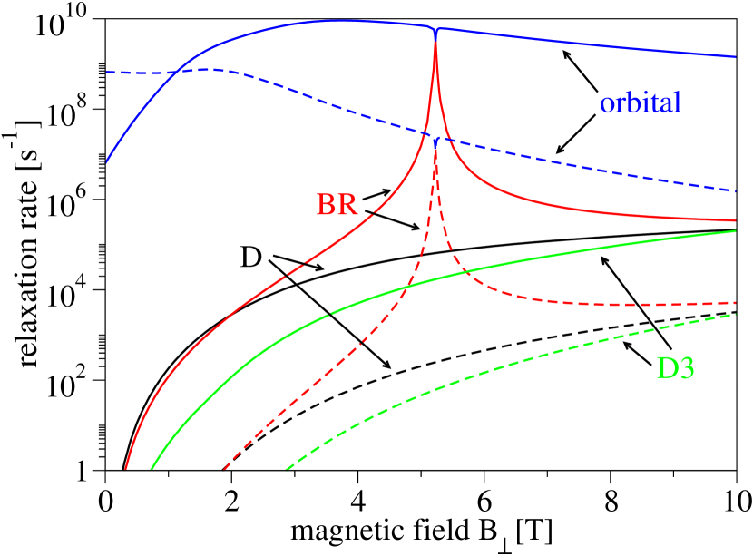
Figure 1: (Color online) Orbital and spin (labels $D,BR,$ and $D3$ denote which spin-orbit interaction is present) relaxation rates in a single quantum dot, for the piezoelectric (solid) and deformation potential (dashed) phonons. The confining length is 32 nm. Anti-crossing of the unperturbed spin and orbital state occurs at $B_{\perp}=5.2$ T.

The orbital relaxation rate is of the order of $10^{9}$ s^-1. The spin-orbit contributions to the rate (not shown in the figure) are of the order of $10^{6}$ s^-1 for the linear spin orbit terms and $10^{5}$ s^-1 for the cubic Dresselhaus term, validating the approximation Eq. (21).

low mag. field	orbital	$\Gamma^{\mathrm{df}}$	$(\pi\gamma_{\mathrm{df}}\hbar^{3}c_{l}/m)l_{0}^{-4}(1-B_{\perp}el_{0}^{2}/2\hbar)$	$\lesssim 0.6$ T
		$\Gamma^{\mathrm{pz}}_{l}$	$(459\pi\gamma_{\mathrm{pz}}c_{l}^{5}m^{5}/4\hbar^{5})l_{0}^{4}(1+5B_{\perp}el_{0}^{2}/2\hbar)$	$\lesssim 0.5$ T
		$\Gamma^{\mathrm{pz}}_{t}$	$(61\pi\gamma_{\mathrm{pz}}c_{l}^{2}c_{t}m^{3}/4\hbar^{3})l_{0}^{2}(1+3B_{\perp}el_{0}^{2}/2\hbar)$	$\lesssim 0.8$ T
	spin	$\Gamma^{\mathrm{df}}$	$(128\pi\gamma_{\mathrm{df}}m^{2}/3\hbar^{7}c_{l}^{3})l_{0}^{8}|\mu B_{\perp}|^{7}l_{D}^{-2}$	$\lesssim 4$ T
		$\Gamma^{\mathrm{pz}}_{l}$	$(128\pi\gamma_{\mathrm{pz}}m^{2}/35\hbar^{7}c_{l}^{3})l_{0}^{8}|\mu B_{\perp}|^{5}l_{D}^{-2}$	$\lesssim 4$ T
		$\Gamma^{\mathrm{pz}}_{t}$	$\Gamma^{\mathrm{pz}}_{l}\times 4c_{l}^{5}/3c_{t}^{5}$	$\lesssim 4$ T
high mag. field	orbital	$\Gamma^{\mathrm{df}}$	$(2\pi\gamma_{\mathrm{df}}\hbar^{13}/3e^{6}m^{5}c_{l}^{3})l_{0}^{-20}B_{\perp}^{-6}$	$\gtrsim 4$ T
		$\Gamma^{\mathrm{pz}}_{l}$	$(8\pi\gamma_{\mathrm{pz}}\hbar^{7}/35e^{4}m^{3}c_{l}^{3})l_{0}^{-12}B_{\perp}^{-4}$	$\gtrsim 4$ T
		$\Gamma^{\mathrm{pz}}_{t}$	$\Gamma^{\mathrm{pz}}_{l}\times 4c_{l}^{5}/3c_{t}^{5}$	$\gtrsim 6$ T
	spin	$\Gamma^{\mathrm{df}}$	$(32\pi\gamma_{\mathrm{df}}|{\mu}|^{5}/3\hbar e^{2}c_{l}^{3})B_{\perp}^{3}l_{D}^{-2}$	$\gtrsim 8$ T
		$\Gamma^{\mathrm{pz}}_{l}$	$(32\pi\gamma_{\mathrm{pz}}|{\mu}|^{3}/35\hbar e^{2}c_{l}^{3})B_{\perp}l_{D}^{-2}$	$\gtrsim 7$ T
		$\Gamma^{\mathrm{pz}}_{t}$	$\Gamma^{\mathrm{pz}}_{l}\times 4c_{l}^{5}/3c_{t}^{5}$	$\gtrsim 7$ T

Table 2: Approximate orbital and spin (due to Dresselhaus coupling) relaxation rates in a single quantum dot at low and high magnetic fields in lowest order of the non-degenerate perturbation theory. In the last column we state the maximal or minimal magnetic field by requiring that at $l_{0}=32$ nm the presented approximation does not differ from the numerical value by more than a factor of 2.

The energy difference of the orbital and the ground state is $E=\hbar^{2}/2ml_{B}^{2}-(\hbar e/2m)B_{\perp}$. At low magnetic fields the high $\mathcal{E}$ limit applies and the deformation potential dominates the orbital relaxation rate. The results are listed in Tab. 2. The values at zero magnetic field, up to a numerical factor, follow from Tab. 1, if one uses $A=1$ and the low magnetic field limits, where $E\approx\hbar^{2}/ml_{0}^{2}$, and $l_{B}\approx l_{0}$. The dependence of the rates on the energy difference of the states, shown in Tab. 1, is enough to understand the different dependence of the deformation and piezoelectric contributions to the orbital relaxation rate at low magnetic fields shown in Figs. 1 and 2. The deformation contribution drops with increasing both the magnetic field and confinement lengths, while the piezoelectric contribution increases with increase of these two parameters.

For fields lower that 1 T the dominant deformation contribution manifest itself on Fig. 2. At magnetic fields higher than 1 T the piezoelectric contribution dominates. Up to about 4 T we are still in the regime $\mathcal{E}\gg 1$ and the rate grows with increasing magnetic field and increasing confinement length. Since the energy difference $E$ drops with increasing magnetic field, for magnetic fields $\gtrsim 6$ T we get into the limit $\mathcal{E}\ll 1$. The corresponding orbital relaxation rates in 2 then follows from Tab. 1 using $A=1$ and high magnetic field limits, where $E\approx\hbar^{3}/emBl_{0}^{4}$ and $l_{B}^{2}\approx 2\hbar/eB$. This leads to a much stronger drop of the deformation contribution to the rate with the increase of both magnetic field and the confinement length, than is the drop of the piezoelectric contribution.

Finally, we explain the influence of the anti-crossing on the orbital relaxation rate, seen in Fig. 1. The anti-crossing contributes by an overall factor of $|\beta_{ii}|^{2}$, see Eq. (14), which multiplies the orbital relaxation rates listed in Tab. 2. Solving the appropriate secular equation, we getBulaev and Loss (2005)

$$|\beta_{ii}|^{2}=\frac{1}{2}+\frac{E}{2\sqrt{E^{2}+|C|^{2}}},$$ (27)

where $E=\hbar^{2}/2ml_{B}^{2}-(\hbar e/2m)B_{\perp}-2\mu B_{\perp}$ is the energy difference between the crossing states, and $C=-\frac{\hbar^{2}}{ml_{B}l_{BR}}(1-B_{\perp}el_{B}^{2}/2\hbar)$ is the strength of the coupling between these states due to the Bychkov-Rashba term. Away from anti-crossing $\beta_{ii}\approx 1$, while directly at the anti-crossing the rate is reduced by a factor of 2. The anti-crossing region for the orbital relaxation is rather narrow ($\sim$ 0.1 T) and manifests itself as a narrow line of the suppression of the rate in Fig. 2.

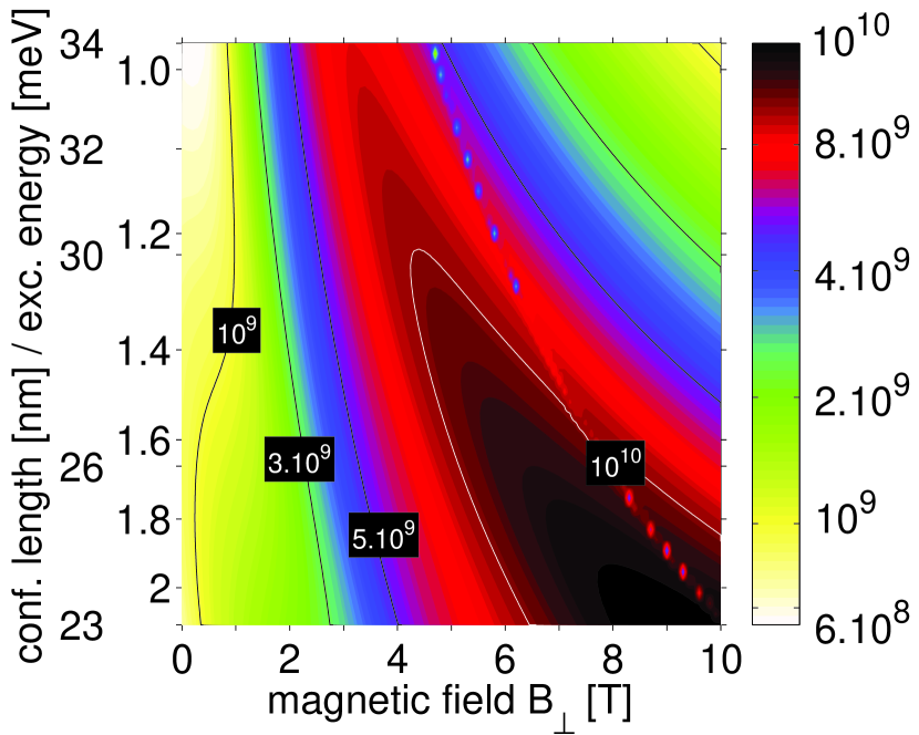
Figure 2: (Color online) Orbital relaxation rate (the sum of the deformation and piezoelectric contribution) in a single quantum dot ‘as a function of magnetic field and the confinement length $l_{0}$ / the confinement (excitation) energy $E_{0}$. The rate is given on the logarithmic scale in the units of s^-1. The solid lines represent equal relaxation rates (equirelaxation lines). The granular structure in the figure is an artifact of the limited data resolution.

III.2.2 Spin relaxation rates

For spin relaxation the relevant energy difference is the Zeeman splitting, $E\approx 2|\mu B|$. Therefore the low energy limit, $\mathcal{E}\ll 1$, applies up to rather high magnetic fields ($\sim$10 T). Piezoelectric transversal phonons dominate the rate. The linear spin-orbit terms dominate over the cubic Dresselhaus term, although the difference becomes smaller for higher magnetic fields. We use an example of the linear Dresselhaus term for analytical expressions. Using Eq. (22) and the limits of low and high magnetic fields we present the analytical spin relaxation rates in Tab. 2 (these results were also derived in Refs. Bulaev and Loss, 2005 and Khaetskii and Nazarov, 2001). These formulas approximately follow from Tab. 1 using $A=|\mu B_{\perp}|l_{B}/l_{D}\delta E$ and $E=|\mu B_{\perp}|$, while noting that $\delta E=E_{0}$ for low and $\delta E=|\mu B_{\perp}|$ for high magnetic fields. The trends described by the Dresselhaus contribution can be seen in Fig. 1. The spin relaxation rate grows much steeper with increasing magnetic field at low $B_{\perp}$ (fifth power) than at high $B_{\perp}$ (first power). Interestingly, at high magnetic fields the rate does not depend on the confining length.

Away from anti-crossing analogous formulas, up to a numerical factor, as those listed in Tab. 2, hold for the contribution to the spin relaxation due to the Bychkov-Rashba term after the substitution $l_{D}\to l_{BR}$. In this case the contribution to the overlap between the spin and ground states due to the term $\beta_{ij}$ in Eq. (14) is negligible. However, comparing the analytical formulas from Tab. 2 with the numerical calculation in Fig. 3, we find discrepancy, except at low magnetic fields. This is because, as can be seen also in Fig. 1, the rate is actually dominated by a spin hot spot (anti-crossing). The anti-crossing occurs for single dots only when the Bychkov-Rashba term is present, since the Dresselhaus terms do not couple the unperturbed orbital states.Bulaev and Loss (2005); Stano and Fabian (2005b) In this case we can neglect all terms but that one containing $\beta_{ij}$ in Eq. (14) and for the spin relaxation rate due to the anti-crossing one gets $\Gamma({\rm spin,acr})=|\beta_{ij}|^{2}\Gamma({\rm orbital})$. The secular equation gives

$$|\beta_{ij}|^{2}=\frac{1}{2}-\frac{E}{2\sqrt{E^{2}+|C|^{2}}},$$ (28)

where the variables are those defined under Eq. (27). Thus, the anti-crossing effectively mixes what we usually call spin and orbital rates. The spin relaxation rate has a sharp peak at the anti-crossing. With increasing the “distance” from the anti-crossing the rate drops, mirroring the drop of the coefficient $|\beta_{ij}|^{2}$. Only far enough from the anti-crossing the term $\beta_{ij}$ is negligible in Eq. (14) and the rate is described by expressions analogous to those from Tab. 2. In Fig. 1 the Bychkov-Rashba contribution to the spin relaxation rate is dominated by the $\beta_{ij}$ term unless the magnetic field is smaller that 2 T. Similarly in Fig. 2, for fields higher than 2 T the total spin relaxation rate is dominated by the anti-crossing contribution due to Bychkov-Rashba term. Consequently, the influence of the anti-crossing is substantial in a much larger region (several Tesla) than in the case of the orbital relaxation.

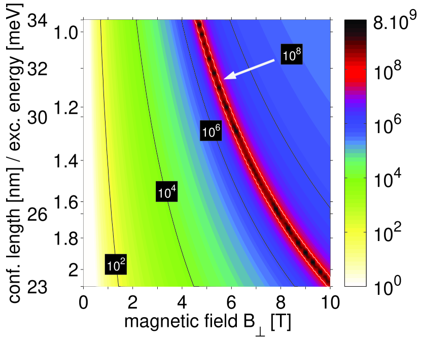
Figure 3: (Color online) Spin relaxation rate in a single quantum dot as a function of magnetic field and the confinement length $l_{0}$ / the confinement energy $E_{0}$. The rate is given on the logarithmic scale in the units of s^-1. The solid lines represent equirelaxation lines.

In Ref. Bulaev and Loss, 2005 spin relaxation rates due to the deformation potential were computed in the lowest order of the perturbation theory and an analogous figure to our Fig. 1 was presented. Our results for both orbital and spin relaxation rates are in a quantitative agreement.

IV Double dots

In our double dot potential the ground (excited orbital) state can be approximated as a symmetric (antisymmetric) combination of two Fock-Darwin functions, $\Psi_{0,0,\uparrow}$, placed at the two potential minima. In Ref. Stano and Fabian, 2005b we have studied the energy spectrum and classified the symmetries of the states of a double dot with a potential given by Eq. (2). What we call here ground, spin and orbital state is denoted there as $\Gamma_{S}^{\uparrow},\,\Gamma_{S}^{\downarrow},$ and $\Gamma_{A}^{\uparrow}$, respectively. The upper index indicates spin and the lower index indicates the symmetry of a particular state with respect to spatial inversion. The energy difference between the ground and excited orbital state, 2$\delta E_{t}$, is strongly influenced by the ratio of the interdot distance and the effective length,Stano and Fabian (2005b) $\mathcal{D}=d/l_{B}$,

$$2\delta E_{t}=\frac{\hbar^{2}}{ml_{B}^{2}}\frac{2\mathcal{D}(1-\theta^{2})\{1+\mathcal{D}\sqrt{\pi}\mathrm{Erfc}(\mathcal{D})-e^{-\mathcal{D}^{2}}\}}{\sqrt{\pi}\{e^{\mathcal{D}^{2}(1+\theta^{2})}-e^{-\mathcal{D}^{2}(1+\theta^{2})}\}},$$ (29)

where a dimensionless parameter $\theta=B_{\perp}el_{B}^{2}/2\hbar$. The tunneling energy $\delta E_{t}$ gives the frequency of single-electron coherent oscillations between the left and right dots. The approximation of Eq. (22) for spin relaxation is correct also here, since Eqs. (9) and (10) do not couple any two of the ground, spin, and orbital states due to a definite symmetry of the $L_{z}$ operator.Stano and Fabian (2005b) There is a coupling through higher excited states with appropriate symmetry, but, as we learn from numerics, this is negligible.

IV.1 In-plane magnetic field

The spin relaxation rate as a function of in-plane magnetic field and the interdot distance is plotted in Fig. 4. The rates for small interdot distances are similar to the single dot case, where the rate grows with increasing magnetic field; for low magnetic fields more steeply than for large. The order of magnitude of the rate is given by Eq. (23), being about $10^{2}$ s^-1 at 1 T and 10⁵ s^-1 at 10 T. At large interdot distances the rate is strongly influenced by the presence of a anti-crossing (spin hot spot), which occurs when the Zeeman and twice the tunneling energies are equal.Stano and Fabian (2005a) If the tunneling energy is changed from zero to a value of order of the single dot excitation energy, regardless of the magnetic field strength, one always passes through a spin hot spot region, where the spin relaxation is very fast. Fortunately there exist specific orientations of the double dot system and the magnetic field, where this anti-crossing does not occur. We call such a configuration “easy passage.”Stano and Fabian (2005a)

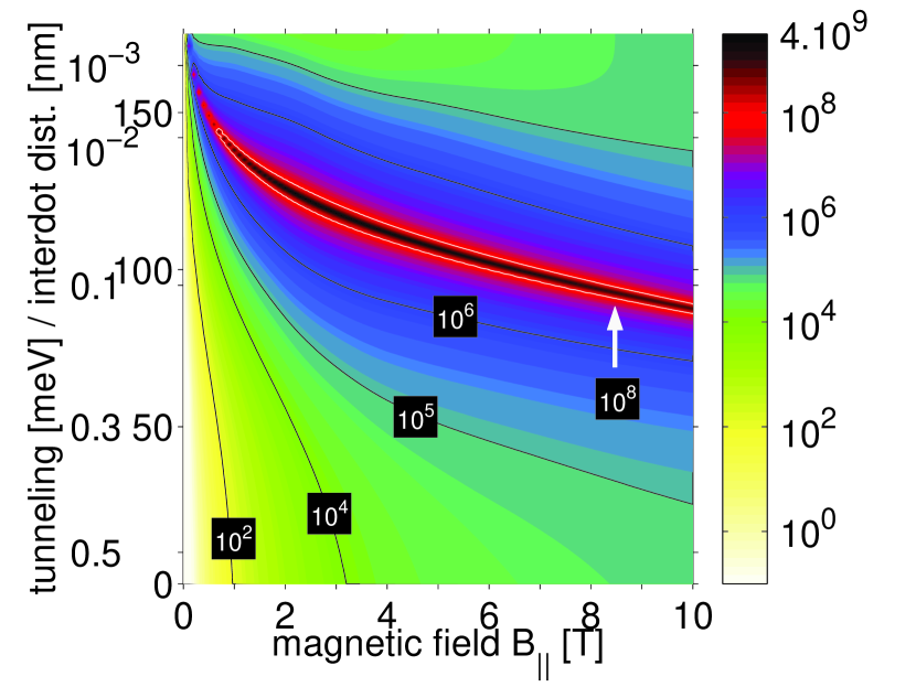
Figure 4: (Color online) Spin relaxation rate in a double quantum dot as a function of in-plane magnetic field for $\gamma=0^{\circ}$ and the interdot distance $d$ / tunneling energy $\delta E_{t}$, for a confinement length 32 nm. The relaxation rate is given on the logarithmic scale in the units of s^-1. The double dot is oriented along [100] ($\delta=0^{\circ}$).

To understand the angular dependence of the rate presented in Ref. Stano and Fabian, 2005a and find conditions for an easy passage we transform the Hamiltonian (6) with $H_{1}$ given by Eq. (22) into coordinates in which the new x axis lies along the dot’s axis $\mathbf{d}$. Since there are no orbital effects in in-plane magnetic fields, in these new coordinates the unperturbed solutions of the Hamiltonian $H_{0}$ have a definite symmetry under inversions about $\hat{x}$ – the ground and spin states are symmetric, while the orbital state is antisymmetric. The transformed $H_{1}$ of Eq. (22), is

$$\begin{split}H_{1}=&-\mu B_{\parallel}\sigma_{z}\large\{x[l_{BR}^{-1}\cos(\gamma-\delta)-l_{D}^{-1}\sin(\gamma+\delta)]\\ &+y[l_{BR}^{-1}\sin(\gamma-\delta)-l_{D}^{-1}\cos(\gamma+\delta)]\large\}.\end{split}$$ (30)

In the single dot case the coefficient $A^{2}$ in Tab. 1 is proportional to the sum of the squared couplings in Eq. (30) at $x$ and $y$. However, in the double dot case, $x$ and $y$ can couple states differently. For large interdot distances the most important influence on the spin relaxation comes from the anti-crossing of the spin and orbital states, which are coupled by terms with the x-like symmetry. Thus, the anti-crossing will not occur if

$$l_{BR}^{-1}\cos(\gamma-\delta)-l_{D}^{-1}\sin(\gamma+\delta)=0.$$ (31)

The angles $\gamma$ and $\delta$ that satisfy the above equation define an easy passage. For a double dot oriented along [100] direction ($\delta=0$) the easy passage occurs for an in-plane magnetic field oriented along angle $\gamma$ given by $\tan\gamma=l_{D}/l_{BR}$. Similarly to the single dot case, the measured angular dependence recovers the ratio of the spin-orbit couplings. Now also revealing which one is larger. More important, as can be seen from Eq. (31), both linear Bychkov-Rashba and Dresselhaus (also cubic) spin-orbit terms contribute to the anti-crossing; in single dots it is only the Bychkov-Rashba coupling which gives relevant spin hot spots. The position of the easy passage is then given by an interplay of all the spin-orbit terms. If the double dot is oriented along [110] ($\delta=\pi/4$), the condition for the easy passage is $\gamma=135^{\circ}$, being independent on the spin-orbit couplings. The importance of this result has been pointed already in Ref. Stano and Fabian, 2005a, where the corresponding numerical results are presented.

IV.2 Perpendicular magnetic field

IV.2.1 Orbital relaxation rate

There are two different regimes for the orbital relaxation, depending on the energy difference of the ground and orbital states, $E=2\delta E_{t}$, which is more sensitive to the interdot distance than to the confinement length. If $\mathcal{D}\equiv d/l_{B}\ll 1$, then $E\approx\hbar^{2}/ml_{B}^{2}$, decreasing with increasing the magnetic field or the interdot distance. The limit of high $\mathcal{E}$ applies and the rates are comparable to the single dot case. On the other hand, if $\mathcal{D}\gg 1$ the energy, and thus also the rates, drop exponentially with increasing the magnetic field or the interdot distance. Due to the complex interplay of the magnetic field and interdot distance, no power law dependence of the rates on magnetic field can be identified. However, approximations in Tab. 1 give analytical formulas with a fair agreement with numerics, if the energy difference $E\approx 2\delta E_{t}$ which is given by Eq. (29).

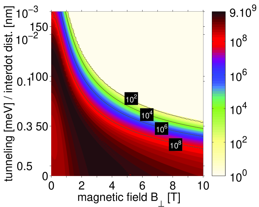
Figure 5: (Color online) Orbital relaxation rate in a double quantum dot as a function of in-plane magnetic field for $\gamma=0^{\circ}$ and the interdot distance $d$ / tunneling energy $\delta E_{t}$, for a confinement length 32 nm. The relaxation rate is given on the logarithmic scale in the units of s^-1. The double dot is oriented along [100] ($\delta=0^{\circ}$).

The dependence of the orbital relaxation rate on the magnetic field and the interdot distance, for a confining length 32 nm, is shown in Fig. 5. The lower left corner is the regime of the high $\mathcal{E}$ limit. The rate here is similar to the single dot case. The opposite corner is the regime of an exponentially small energy difference and the rate is practically zero. The transition between these two regimes comes for a smaller interdot distance if the magnetic field is higher, since the transition occurs when $d\sim l_{B}$. Again, as in the single dot case, the anti-crossing does not have a large influence on the orbital rate – in the figure it can hardly be seen. For interdot distances much larger than $l_{B}$ the dots are effectively isolated.

IV.2.2 Spin relaxation rate

Spin relaxation in double dots reveals a surprising complexity as compared to the single dot case. The complexity is due to the strong anisotropy of spin hot spots. While anisotropy appears already in single dots, caused by the interference of the Bychkov-Rashba and Dresselhaus couplings, additional anisotropy appears in spin hot spots. This anisotropy does not require the presence of both couplings. Instead, it is caused by the selection rules for spin-orbit virtual transitions in the double-dot spectrum. The corresponding physics is described by the transformed Hamiltonian $H_{1}$ of Eq. 30. We have presented the corresponding numerical calculation in Ref. Stano and Fabian, 2005a. Here we discuss the individual contributions of the Bychkov-Rashba and Dresselhaus terms in the spin relaxation rate and, specifically, in the spin hot spot anisotropy.

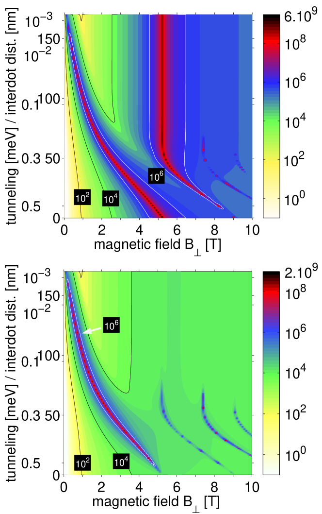
Figure 6: (Color online) Spin relaxation rate as a function of perpendicular magnetic field for $\gamma=0^{\circ}$ and the interdot distance $d$ / tunneling energy $\delta E_{t}$ (at zero magnetic field only), for a confinement length 32 nm. The relaxation rate is given in logarithmic scale in the units of s^-1. The double dot is oriented along [100] ($\delta=0^{\circ}$). The upper figure shows results when only the Bychkov-Rashba term is present in the Hamiltonian. In the lower figure, only the Dresselhaus terms are present.

The contribution to the spin relaxation rate from the Bychkov-Rashba (Dresselhaus) term is shown in the upper (lower) part of Fig. 6. The changes of the upper figure, if the Dresselhaus terms were present, would be very small (compare with Fig. 2 in Ref. Stano and Fabian, 2005a). For low magnetic fields the rate grows with increasing magnetic field, as we expect from Tab. 1. However, similarly to the in-plane magnetic field case, the spin hot spots (ridges in Fig. 6) dominate the rate for most of the parameters’ range. The interdot distance strongly influences the spin relaxation rate by determining the position of anti-crossings. In high magnetic fields, the spin state can anti-cross higher orbital states depending on the symmetry of these states. However, the influence of these anti-crossings on the rate is limited to a narrow region of magnetic fields, since the dots are effectively isolated at high fields and the crossing states do not comply with the selection rules for spin-orbit couplings of single dot states.

It is interesting to compare the contribution to the spin relaxation by the Bychkov-Rashba and the Dresselhaus terms. Let us first look at the single dot regime, which in Fig. 6 is visible at $d=0$. The spin hot spot appears only for the Bychkov-Rashba coupling, in line with our earlier observation Stano and Fabian (2005b). The Dresselhaus coupling becomes effective only in the coupled-dot system in which the symmetry of the lowest orbital states allows the coupling at the level crossings. The coupling is again absent at two isolated dots ($d\to\infty$). Another nice feature seen in Fig. 6 is the transformation of the single-dot spin hot spot at about 5 T to a double-dot spin hot spot at lower fields, while the single-dot spin hot spot that starts at about 9 T shifts towards 5 T in the double dot and remains there at all couplings.

Similarly to the in-plane field case, we can understand the anisotropy of the spin relaxation in perpendicular magnetic field by transforming the Hamiltonian of Eq. (22) into a coordinate system with the x-axes being along $\mathbf{d}$:

$$\begin{split}H_{1}=&\mu B_{\perp}\large\{x[\sigma_{x}(l_{BR}^{-1}-l_{D}^{-1}\sin 2\delta)-\sigma_{y}l_{D}^{-1}\cos 2\delta]\\ &+y[\sigma_{y}(l_{BR}^{-1}+l_{D}^{-1}\sin 2\delta)-\sigma_{x}l_{D}^{-1}\cos 2\delta]\large\}.\end{split}$$ (32)

Due to the presence of the orbital effects of the perpendicular magnetic field, the unperturbed states have no specific symmetry under inversions along $x$. As a result only in the limit of low magnetic fields ($l_{B}\approx l_{0}$), for us below 1 T, the term in Eq. (32) containing $x$ dominates over the term containing $y$; in higher fields both terms contribute. In this limit the condition for a suppression of the anti-crossing is $l_{D}=l_{BR}$ and $\delta=45^{\circ}$. This we call a “weak passage”, since the anti-crossing, while strongly suppressed, is still present. If the condition for a weak passage is not fulfilled, the spin relaxation rate, as a function of $\delta$, still has a minimum at $\delta=45^{\circ}$ and a maximum at $\delta=135^{\circ}$. However, the ratio between the two extremal values is in general of order 1.

IV.3 Other growing directions

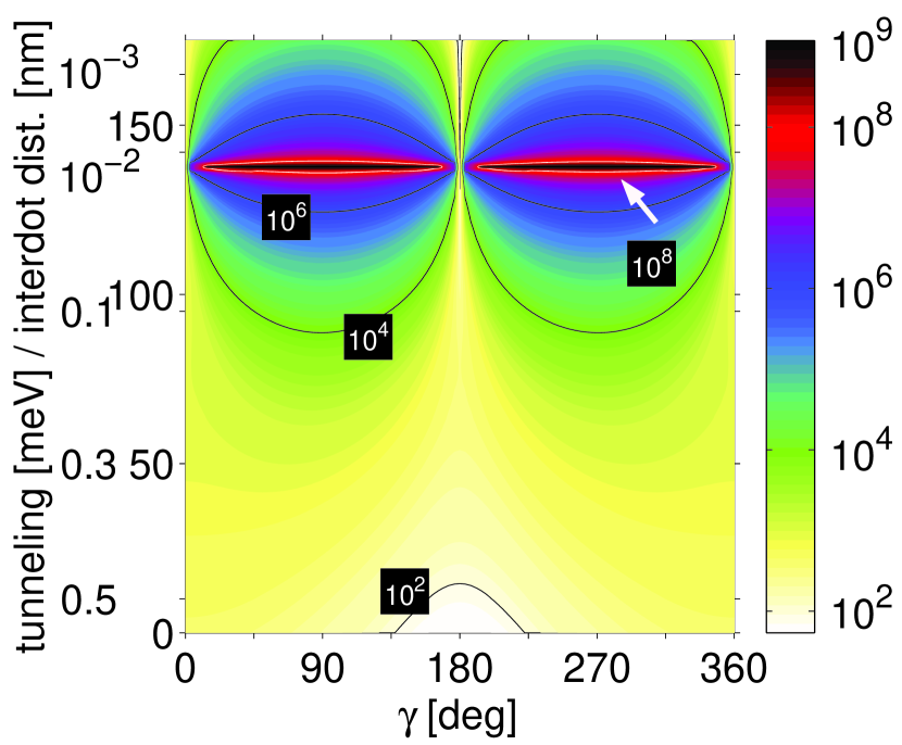
Figure 7: (Color online) Spin relaxation rate as a function of $\gamma$ and the tunneling energy for $B_{||}=1$ T, for [110] growing direction. The dot orientation is given by $\delta=\pi/2$. The relaxation rate is given in logarithmic scale in the units of s^-1.

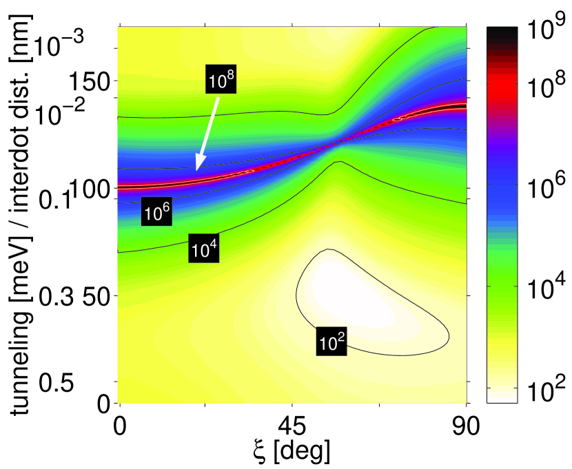
Figure 8: (Color online) Spin relaxation rate as a function of $\xi$ and tunneling energy for $B=1$ T, for [110] growing direction. The dot orientation is given by $\delta=\pi/2$. The relaxation rate is given in logarithmic scale in the units of s^-1.

Thus far we have considered lateral quantum dots defined in a (001) plane of a GaAs heterostructure. A different growing direction leads to a different form of the Dresselhaus spin-orbit interactionsŽutić et al. (2004) (the form of the Bychkov-Rashba term remains unchanged) and to different conditions for the easy passage. Our results are summarized in Tab. 3. For the [111] growth direction the Dresselhaus term has the same form as the Bychkov-Rashba one. Our results easily translate for this case by placing formally $l_{D}\to\infty$. There will be no spin relaxation anisotropy in single dots, while in double dots spin hot spots vanish for $\cos(\gamma-\delta)=0$ at in-plane fields. For a general magnetic field a weak passage occurs only at specific spin-orbit parameters, given by $2\sqrt{3}l_{BR}+l_{D}=0$ (the couplings can be negative).

growing dir.	in-plane	general
$[001]$	$l_{BR}\cos(\gamma+\delta)=\phantom{eee}$	$l_{D}=l_{BR},\,\delta=\pi/4$
	$\phantom{eee}=l_{D}\sin(\gamma-\delta)$
$[111]$	$\cos(\gamma-\delta)=0$	$2\sqrt{3}l_{BR}+l_{D}=0$
$[110]$	$\gamma=0,\,\delta=\pi/2$	$l_{BR}\cos\delta=\pm 2l_{D}\cot\xi,$
		$\sin(\delta-\gamma)=\pm 1$
$[\cos\alpha\,\sin\alpha\,0]$	$\delta=\pi/2,$	$l_{D}=-l_{BR}\cos 2\alpha,$
	$l_{D}\tan\gamma=-l_{BR}\cos 2\alpha$	$\delta=\pi/4,\,\xi=0$

Table 3: Easy passage conditions for several growing directions in an in-plane magnetic field and weak passage conditions for a magnetic field with a nonzero perpendicular component. The $z$-axis points in the growth direction. The angle between $\mathbf{d}$ and the (accordingly rotated) $x$-axis is $\delta$, the angle between the in-plane part of the magnetic field and the $x$-axis is $\gamma$, while $\xi$ is the angle between the magnetic field and the $z$-axis.

A less trivial situation occurs for the [110] grown quantum well. The linear Dresselhaus coupling has the form

$$H_{D}=-\frac{\hbar}{4ml_{D}}\sigma_{z}P_{x}$$ (33)

Unlike the Bychkov-Rashba coupling, which has eigenspins always in the plane, the [110] Dresselhaus term has eigenspins oriented out of the plane.

The calculated spin relaxation rate for the double dot system oriented along $\delta=\pi/2$ in an in-plane magnetic field of $B_{||}=1$ T is shown in Fig. 7. The spin hot spots exist for all orientations of the field except at multiples of $\pi$. This is confirmed by analytical considerations summarized in Tab. 3. The easy passage exists if the dot is oriented along the (rotated) x axis, while the in-plane magnetic field is along $\hat{y}$. Also, the [110] Hamiltonian is not invariant under the in-plane inversion of the coordinates which is why the period in $\gamma$ for the relaxation rate is twice as in the case of the [001] growing direction. However, the part of the Hamiltonian important for anti-crossing is invariant with respect to inversion along $\hat{y}$. Therefore, the results in Fig. 7 for $\gamma>\pi$ are equal to those at $2\pi-\gamma$ to a very good approximation.

In order to demonstrate the difference between easy and weak passages, we plot in Fig. 8 the calculated spin relaxation rate in double dots defined in a (110) plane. The dots are oriented along $\hat{y}$. From Tab. 3 one gets the conditions for the weak passage to be $\gamma=0$, and, for our spin-orbit couplings, $\xi=56^{\circ}$, where $\xi$ is the angle between the magnetic field and $\hat{z}$. This arrangement corresponds to the “neck” on the spin hot spot in Fig. 8. However, contrary to an easy passage, here the width of the anti-crossing region is finite and gets larger with increasing magnetic field (not shown). Since all weak passages we found depend on spin-orbit couplings, they (better, the corresponding geometries) are much less useful for robust inhibiting of spin relaxation than easy passages.

In the above analysis we have not considered the cubic Dresselhaus term, $H_{D3}$, in deriving the conditions for easy passages. Being cubic, even after rotating the double dot ($\delta\neq 0$), it always has qualitatively the same symmetry properties with respect to inversions about $\hat{x}$ and $\hat{y}$ – it is a sum of two terms, one with symmetry of $x$ and one $y$. Therefore the presence of $H_{D3}$ does not destroy the easy passage. It can only slightly change the conditions for the easy passage to occur. For our parameters this change, checked numerically, is only on the order of $1^{\circ}$ for the of angles in Tab. 3, so the linear terms should provide a realistic guidance to experimental demonstrations of the predicted anisotropy.

V Conclusions

We have calculated phonon-induced orbital and spin relaxation rates of single electron states in single and double quantum dots. The rates were calculated as a function of in-plane and perpendicular magnetic fields, as well as a function of the field and (in the case of double dots) dots’ orientation. Realistic, GaAs defined, electron-phonon piezoelectric and deformation potential Hamiltonians were considered. Similarly, relevant spin-orbit interactions, namely the Bychkov-Rashba and linear and cubic Dresselhaus couplings, were used to calculate the spin relaxation rate. We have supported our numerical findings by analytical models based on perturbation theory, deriving effective Hamiltonians which display, in the lowest order, all the important effects seen in numerics. We have proposed using a classifying dimensionless parameter $\mathcal{E}$ which allows to obtain relevant trends and order-of-magnitude estimates in important limiting cases.

In the case of single dots, we have carefully analyzed the theoretically predicted anisotropy of the spin relaxation rate in an in-plane magnetic field. The anisotropy comes from the interplay of the linear Bychkov-Rashba and Dresselhaus terms (if only one of the terms dominates, the anisotropy is absent). Experimental verification of the anisotropy would give a strong evidence of the spin-orbit mechanism of spin relaxation. Furthermore, such a measurement would enable to estimate the ratio of the two relevant spin-orbit terms.

For single dots in a perpendicular magnetic field, which causes cyclotron effects as well as Zeeman splitting, we have numerically investigated the orbital relaxation rate. In addition, we have provided a simple analytical scheme to estimate the rates in the important limits of low and high magnetic fields, and found the corresponding rate as a function of the confining length. The orbital relaxation rate is found to be of the order of $10^{9}$ s^-1, with a relatively small dependence on the magnetic field. At anti-crossings the orbital relaxation rate is reduced by a factor of two. At low magnetic fields the rate is dominated by the deformation potential electron-phonon interaction, while at high fields it is dominated by piezoelectric phonons.

On the other hand, the spin relaxation in single dots is always dominated by piezoelectric transversal phonons. The contribution of deformation potential phonons is more than a decade smaller. The rate is on the order of $10^{5}$ s^-1 over a large region of parameters (magnetic field and excitation energy). However, the rate is strongly enhanced in the region of anti-crossing/spin hot spot, where it becomes comparable to the orbital relaxation rate. We have also provided analytical estimates of the rate (away from the spin hot spots) for various phonon contributions, at the limits of low and high magnetic fields.

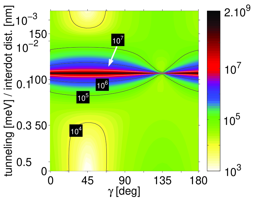
Figure 9: (Color online) Spin relaxation rate in a double dot as a function of the orientation of the in-plane magnetic field and tunneling energy for $B=5$ T, for [001] growing direction. The dot orientation is given by $\delta=\pi/4$. A small asymmetric term is added into the confinement potential (an electric field of $10^{3}$ V/m in $y$ direction is applied in on one of the dots). By this, the easy passage is turned into a weak passage – compare with Fig. 4 in Ref. Stano and Fabian, 2005a.

The physics is more complex in coupled dots. We have numerically studied spin relaxation in double dots in in-plane magnetic fields, in which the rate is strongly anisotropic in the direction of both the magnetic field and the dots’ axis. Similarly to the single dot case, the piezoelectric phonons dominate spin relaxation here. We have demonstrated that a spin-hot spot exists at useful magnetic fields (say, 1 T) and interdot couplings (0.1-0.01 meV). In fact, a spin hot spot is a typical phenomenon in symmetric double dots since it appears when the tunneling (coupling) energy becomes comparable to the Zeeman splitting. Fortunately, the spin hot spots are strongly anisotropic, due to the symmetry of the lowest orbital electronic states, and they vanish at certain orientations of the field and the dots’ axis. We have systematically investigated these “easy passages” using an analytical model. We have found the criteria for the absence of spin hot spots for different growth directions of the underlying quantum well. These criteria should be seriously considered in fabricating double dot systems for spin-based quantum information processing which requires low spin relaxation.

For double dots in a perpendicular magnetic field, the orbital relaxation rate is most influenced by the energy difference of the corresponding coupled states. The energy has a range over eight orders of magnitude due to the cyclotron effects in the interdot coupling. As in the single dot case, both deformation potential and piezoelectric phonons can dominate the orbital relaxation. The spin relaxation in double dots in a perpendicular field has similar qualitative features as in the single dot case, with an additional anisotropy given by the orientation of the double dot with respect to the crystallographic axes. However, unlike in in-plane fields, only weak easy passages (in which spin hot spots form a neck on the parameter map, rather than disappear altogether) exist in a perpendicular magnetic field. We have also observed a nice shift of spin hot spots to the lower field neighbors as the tunneling between the dots decreases. While the perpendicular fields provide a nice opportunity to study fundamental physics of double dot systems, they are less useful in quantum information processing due to the omnipresence of spin hot spots and weak passages.

Our final note concerns the symmetry of the double dot systems investigated in this paper. Do our conclusions hold if the symmetry is broken? The answer is yes, if the double-dot system still possesses either x- or y-like symmetry. Suppose, for example, that a weak electric field is applied along $\hat{x}$ or $\hat{y}$, or one of the dots is somewhat smaller than the other. The spin hot spot anisotropy still leads to easy passages in spin relaxation in in-plane magnetic fields. On the other hand, if the symmetry breaking is $xy$-like (an electric field pointing along a diagonal, for example), the easy passage is destroyed since the selection rules for the lowest orbital states will allow coupling of the states by the term containing $y$ in $H_{1}$ of Eq. 30 (recall that it was the vanishing of the term containing $x$ that lead to the appearance of easy passages). This situation is demonstrated in Fig. 9. A double dot system in an in-plane field of 5 T is oriented along [110] (the growth direction is [001]). If the double dot is symmetric, an easy passage exists for $\gamma=135^{\circ}$ (the corresponding figure is given in Ref. Stano and Fabian, 2005a). However, if one of the dots is subject to a $y$-like electric field, so that the overall symmetry of the perturbation is $xy$-like, the easy passage turns to a weak passage—at all directions of the in-plane magnetic field there exists an interdot coupling in which the spin relaxation rate is greatly enhanced. This is another important message for spin-based quantum information processing in quantum dots.

References

- Žutić et al. (2004) I. Žutić, J. Fabian, and S. Das Sarma, Rev. Mod. Phys. 76, 323 (2004).
- Loss and DiVincenzo (1998) D. Loss and D. P. DiVincenzo, Phys. Rev. A 57, 120 (1998).
- Fabian and Hohenester (2005) J. Fabian and U. Hohenester, Phys. Rev. B 72, 201304(R) (2005).
- Erlingsson et al. (2001) S. I. Erlingsson, Y. V. Nazarov, and V. I. Falko, Phys. Rev. B 64, 195306 (2001).
- Erlingsson and Nazarov (2002) S. I. Erlingsson and Y. V. Nazarov, Phys. Rev. B 66, 155327 (2002).
- Coish and Loss (2005) W. A. Coish and D. Loss, Phys. Rev. B 72, 125337 (2005).
- Khaetskii and Nazarov (2000) A. V. Khaetskii and Y. V. Nazarov, Phys. Rev. B 61, 12639 (2000).
- Khaetskii and Nazarov (2001) A. V. Khaetskii and Y. V. Nazarov, Phys. Rev. B 64, 125316 (2001).
- Falko et al. (2005) V. I. Falko, B. L. Altshuler, and O. Tsyplyatyev, Phys. Rev. Lett. 95, 076603 (2005).
- Aleiner and Faľko (2001) I. Aleiner and V. I. Faľko, Phys. Rev. Lett. 87, 256801 (2001).
- Alcalde et al. (2004) A. M. Alcalde, Q. Fanayo, and G. E. Marques, Physica E 20 (2004).
- Destefani et al. (2004) C. F. Destefani, S. E. Ulloa, and G. E. Marques, Phys. Rev. B 69, 125302 (2004).
- Stavrou and Hu (2005) V. N. Stavrou and X. Hu, Phys. Rev. B 72, 075362 (2005).
- Fedichkin and Fedorov (2004) L. Fedichkin and A. Fedorov, Phys. Rev. A 69, 032311 (2004).
- San-Jose et al. (2006) P. San-Jose, G. Zarand, A. Shnirman, and G. Schön, cond-mat/0603847 (2006).
- Florescu and Hawrylak (2006) M. Florescu and P. Hawrylak, Phys. Rev. B 73, 045304 (2006).
- Wang and Wu (2006) Y. Y. Wang and M. W. Wu, cond-mat/0601028 (2006).
- Cheng et al. (2004) J. L. Cheng, M. W. Wu, and C. Lü, Phys. Rev. B 69, 115318 (2004).
- Romano et al. (2005) C. L. Romano, P. I. Tamborenea, and S. E. Ulloa, cond-mat/0508303 (2005).
- Woods et al. (2002) L. M. Woods, T. L. Reinecke, and Y. Lyanda-Geller, Phys. Rev. B 66, 161318(R) (2002).
- Alcade et al. (2005) A. M. Alcade, O. O. Diniz Neto, and G. E. Marques, Microel. Jour. 36, 1034 (2005).
- Sherman and Lockwood (2005) E. Y. Sherman and D. J. Lockwood, Phys. Rev. B 72, 125340 (2005).
- Calero et al. (2005) C. Calero, E. M. Chudnovsky, and D. A. Garanin, Phys. Rev. Lett. 95, 166603 (2005).
- Semenov and Kim (2004) Y. G. Semenov and K. W. Kim, Phys. Rev. Lett. 92, 026601 (2004).
- Golovach et al. (2004) V. N. Golovach, A. Khaetskii, and D. Loss, Phys. Rev. Let. 93, 16601 (2004).
- Hu and Das Sarma (2006) X. Hu and S. Das Sarma, Phys. Rev. Lett. 96, 100501 (2006).
- Hanson et al. (2003) R. Hanson, B. Witkamp, L. M. K. Vandersypen, L. H. Willems van Beveren, J. M. Elzerman, and J. P. Kouwenhoven, Phys. Rev. Lett. 91, 196802 (2003).
- Hanson et al. (2005) R. Hanson, L. H. Willems van Beveren, I. T. Vink, J. M. Elzerman, and L. M. K. Vandersypen, Phys. Rev. Lett. 94, 196802 (2005).
- Elzerman et al. (2004) J. M. Elzerman, R. Hanson, L. H. Willem van Beveren, B. Witkamp, L. M. K. Vandersypen, and L. P. Kouwenhoven, Nature 430, 431 (2004).
- Fujisawa et al. (2002a) T. Fujisawa, D. G. Austing, Y. Tokura, Y. Hirayama, and S. Tarucha, Nature 419, 278 (2002a).
- Fujisawa et al. (2002b) T. Fujisawa, Y. Tokura, D. G. Austing, Y. Hirayama, and S. Tarucha, Physica B 314, 224 (2002b).
- Kroutvar et al. (2004) M. Kroutvar, Y. Ducommun, D. Heiss, M. Bichler, D. Schuh, G. Absteiter, and J. J. Finley, Nature 432, 81 (2004).
- Johnson et al. (2005) A. C. Johnson, J. R. Petta, J. M. Taylor, A. Yacobi, M. D. Lukin, C. M. Marcus, M. P. Hanson, and A. C. Gossard, Nature 435, 925 (2005).
- Sasaki et al. (2005) S. Sasaki, T. Fujisawa, T. Hayashi, and Y. Hirayama, Phys. Rev. Lett. 95, 056803 (2005).
- Hayashi et al. (2003) T. Hayashi, T. Fujisawa, H. D. Cheong, Y. H. Joeong, and Y. Hirayama, Phys. Rev. Lett. 91, 226804 (2003).
- Petta et al. (2004) J. R. Petta, A. C. Johnson, C. M. Markus, M. P. Hanson, and A. C. Gossard, Phys. Rev. Lett. 93, 186802 (2004).
- Stano and Fabian (2005a) P. Stano and J. Fabian, cond-mat/0512713; Phys. Rev. Lett. (in press) (2005a).
- Fabian and Das Sarma (1998) J. Fabian and S. Das Sarma, Phys. Rev. Lett. 81, 5624 (1998).
- Fabian and Das Sarma (1999) J. Fabian and S. Das Sarma, Phys. Rev. Lett. 83, 1211 (1999).
- Bulaev and Loss (2005) D. V. Bulaev and D. Loss, Phys. Rev. B 71, 205324 (2005).
- Bagga et al. (2006) A. Bagga, P. Pietilainen, and T. Chakraborty, cond-mat/0601390 (2006).
- Stano and Fabian (2005b) P. Stano and J. Fabian, Phys. Rev. B 72, 155410 (2005b).
- Rashba (1960) E. I. Rashba, Fiz. Tverd. Tela (Leningrad) 2, 1224 (1960).
- Bychkov and Rashba (1984) Y. A. Bychkov and E. I. Rashba, J. Phys. C 17, 6039 (1984).
- Dresselhaus (1955) G. Dresselhaus, Phys. Rev. 100, 580 (1955).
- Dyakonov and Kachorovskii (1986) M. Dyakonov and V. Kachorovskii, Fiz. Tekh. Poluprovodn.(S-Petersburg) 20, 178 (1986).
- de Sousa and Das Sarma (2003) R. de Sousa and S. Das Sarma, Phys. Rev B 68, 155330 (2003).
- Miller et al. (2003) J. Miller, D. Zumbuhl, C. Marcus, Y. Lyanda-Geller, D. Goldhaber-Gordon, K. Campman, and A. Gossard, Phys. Rev. Lett. 90, 76807 (2003).
- Knap et al. (1996) W. Knap, C. Skierbiszewski, A. Zduniak, E. Litwin-Staszewska, D. Bertho, F. Kobbi, J. L. Robert, G. E. Pikus, F. G. Pikus, S. V. Iordanskii, et al., Phys. Rev. B 53, 3912 (1996).
- Kainz et al. (2003) J. Kainz, U. Rossler, and R. Winkler, Phys. Rev. B 68, 075322 (2003).
- Fock (1928) V. Fock, Z. Phys. 47, 446 (1928).
- Darwin (1931) C. G. Darwin, Proc. Cambridge Philos. Soc. 27, 86 (1931).
- Mahan (2000) G. D. Mahan, Many-particle physics (Kluwer, New York, 2000).