Approach to jamming in an air-fluidized granular bed

Abstract

Quasi-2D bidisperse amorphous systems of steel beads are fluidized by a uniform upflow of air, so that the beads roll on a horizontal plane. The short-time ballistic motion of the beads is stochastic, with non-Gaussian speed distributions and with different average kinetic energies for the two species. The approach to jamming is studied as a function of increasing bead area fraction and also as a function of decreasing air speed. The structure of the system is measured in terms of both the Voronoi tessellation and the pair distribution function. The dynamics of the system is measured in terms of both displacement statistics and the density of vibrational states. These quantities all exhibit tell-tale features as the dynamics become more constrained closer to jamming. Though the system is driven and athermal, the behavior is remarkably reminiscent of that in dense colloidal suspensions and supercooled liquids.

One of the grand challenges in physics today is to understand non-equilibrium systems, which evolve with time or remain in a steady state by injection of energy. The concept of jamming is helping to unify such seemingly disparate non-equilibrium systems as supercooled liquids and dense collections of droplets, bubbles, colloidal particles, grains, and traffic Cates et al. (1998); Liu and Nagel (1998, 2001). In all cases, the individual units can be jammed – stuck essentially forever in a single packing configuration – by either lowering the temperature, increasing the density, or decreasing the driving. But what changes occur in the structure and dynamics that signal the approach to jamming? Which features are generic, and which depend on details of the system or details of the driving? A priori all non-equilibrium systems are different and all details should matter; therefore, the ultimate utility and universality of the jamming concept is not at all obvious.

Granular materials have a myriad of occurrences and applications, and are being widely studied as idealized non-thermal systems that can be unjammed by external forcing Nedderman (1992); Jaeger et al. (1996); Duran (2000). Injection of energy at a boundary, either by shaking or shearing, can induce structural rearrangements and cause the grains to explore different packing configurations; however, the microscopic grain-scale response is not usually homogeneous in space or time. This can result in fascinating phenomena such as pattern formation, compaction, shear banding, and avalanching, which have been explained by a growing set of theoretical models with disjoint underlying assumptions and ranges of applicability. To isolate and identify the universally generic features of jamming behavior it would be helpful to explore other driving mechanisms, where the energy injection is homogeneous in space and time. One approach is gravity-driven flow in a vertical hopper of constant cross-section, where flow speed is set by bottom opening. Diffusing-wave spectroscopy and video imaging, combined Menon and Durian (1997), reveal that the dynamics are ballistic at short times, diffusive at long times, and subdiffusive at intermediate times when the grains are ‘trapped’ in a cage of nearest neighbors. Such a sequence of dynamics is familiar from thermal systems of glassy liquids and dense colloids Liu and Nagel (2001). Another approach is high-frequency vertical vibration of a horizontal granular monolayer. For dilute grains, this is found to give Gaussian velocity statistics, in analogy with thermal systems Baxter and Olafsen (2003). For dense monodisperse grains, this is found to give melting and crystallization behavior also in analogy with thermal systems Olafsen and Urbach (2005); Reis et al. (2006).

In this paper, we explore the universality of the jamming concept by experimental study of disordered granular monolayers. To achieve homogeneous energy injection we employ a novel approach in which grain motion is excited by a uniform upflow of air. For dilute grains, the shedding of turbulent wakes was found earlier to cause stochastic motion that could be described by a Langevin equation respecting the Fluctuation-Dissipation Theorem, in analogy with thermal systems Ojha et al. (2004, 2005); Abate and Durian (2005). Now we extend this approach to dense collections of grains. To prevent crystallized domains, and hence to enforce homogeneous disorder, we use a bidisperse mixture of two grain sizes. The extent of grain motion is gradually suppressed, and the jamming transition is thus approached, by both raising the packing fraction and by decreasing the grain speeds in such as way as to approach Point-J O’Hern et al. (2002, 2003) in the jamming phase diagram. For a given state of the system, we thoroughly characterize both structure and dynamics using a broad set of statistical measures familiar from study of molecular liquids and colloidal suspensions. In addition to such usual quantities as coordination number, pair-distribution function, mean-squared displacement, and density of states, we also use more novel tools such as a shape factor for the Voronoi cells and the kurtosis of the displacement distribution. We shall show that the microscopic behavior is not in perfect analogy with thermal systems. Rather, the two grain species have different average kinetic energies, and their speed distributions are not Gaussian. Nevertheless, the systematic change in behavior on approach to jamming is found to be in good analogy with thermal systems such as supercooled liquids and dense colloidal suspensions. Our findings support the universality of the jamming concept, and give insight as to which aspects of granular behavior are generic and which are due to details of energy injection.

I Methods

The primary granular system under investigation consists of a 1:1 bidisperse mixture of chrome-coated steel ball-bearings with diameters of $d_{b}=11/32~{}{\rm inch}=0.873$ cm and $d_{s}=1/4~{}{\rm inch}=0.635$ cm; the diameter ratio is 1.375; the masses are 2.72 g and 1.05 g, respectively. These beads roll on a circular horizontal sieve, which is 6.97 inches in diameter and has a $100~{}\mu$m mesh size. The packing fraction, equal to the fraction of projected area occupied by the entire collection of beads, is varied across the range $0.487<\phi<0.826$ by taking the total number of beads across the range $262<N<444$.

The motion of the beads is excited by a vertical upflow of air through the mesh at fixed superficial speed $950~{}\pm 10$ cm/s. This is the volume per time of air flow, divided by sieve area; the air speed between the beads is greater according to the value of $\phi$. The air speed is large enough to drive stochastic bead motion by turbulence (${\rm Re}\approx 10^{4}$), but is small enough that the beads maintain contact with the sieve and roll without slipping. The uniformity of the airflow is achieved by mounting the sieve atop a $1.5\times 1.5\times 4~{}{\rm ft}^{3}$ windbox, and is monitored by hot-wire anemometer.

The system of beads is illuminated by six 100 W incandescent bulbs, arrayed in a 1 ft diameter ring located 3 ft above the sieve. Specularly reflected light from the very top of each bead is imaged by a digital CCD camera, Pulnix 6710, placed at the center of the illumination ring. The sensing element consists of a $644\times 484$ array of $10\times 10~{}\mu{\rm m}^{2}$ square pixels, 8 bits deep. Images are captured at a frame rate of 120 Hz, converted to binary, and streamed to hard-disk as AVI movies using the lossless Microsoft RLE codec. Run durations are 20 minutes. The threshold level for binary conversion is chosen so that each beads appears as a small blob about 9 and 18 pixels in area for the small and large beads, respectively. Note that the spot size is smaller than the bead size, which aids in species identification and ensures that colliding beads appear well-separated. The minimum resolvable bead displacement, below which there is a fixed pattern of illuminated pixels within a blob, is about 0.1 pixels.

The AVI movies are post-processed using custom LabVIEW routines, as follows, to deduce bead locations and speeds. For each frame, each bead is first identified as a contiguous blob of bright pixels. Bead locations are then deduced from the average position of the associated illuminated pixels. Individual beads are then tracked uniquely vs time, knowing that the displacement between successive frames is always less than a bead diameter. Finally, positions are refined and velocities are deduced by fitting position vs time data to a cubic polynomial. The fitting window is $\pm 5$ points, defined by Gaussian weighting that nearly vanishes at the edges; this choice of weighting helps ensure continuity of the derivatives. The rms deviation of the raw data from the polynomial fits is 0.0035 cm, which corresponds to 0.085 pixels – close to the minimum resolvable bead displacement. The accuracy of the fitted position is smaller according to the number of points in the fitting window: about 0.0035 cm/$\sqrt{5}=0.0016$ cm. This and the frame rate give an estimate of speed accuracy as 0.2 cm/s. An alternative analysis approach is to run the time-trace data through a low pass filter using Fourier methods. We find very similar results to the weighted polynomial fits for a range of cut-off frequencies, as long as the rms difference between raw and filtered data is between about 0.1 and 0.3 pixels. While there is no significant difference in the plots presented below, we slightly prefer the polynomial fit approach based on qualitative inspection – it is much slower but appears better at hitting the peaks without giving spurious oscillations.

II General

For orientation, Fig. 1a shows representative configurations for two area fractions, $\phi=48.7\%$ and $\phi=80.9\%$. To mimic an actual photograph, a disk with the same diameter as the bead has been centered over each bead’s position, with a darker shade for the big beads. Note that the configurations are disordered, and that the two bead species are distributed evenly across the system. With time, due to the upflow of air, the beads move about and explore different structural configurations. Over the duration of a twenty minute run, at our lowest packing fractions, each bead has time to sample the entire cell several times over. The beads never crystalize or segregate according to size. Thus, the system appears to be both stationary and ergodic. However, the beads tend to idle for a while if they come in contact with the boundary of the sieve. Therefore, care is taken to prevent the contamination of bulk behavior by boundary beads.

In the next sections we quantify first structure and then dynamics, and how they both change with increasing packing fraction on approach to jamming. A two-dimensional random close packing of bidisperse hard disks can occupy a range of area fractions less than about 84%, depending on diameter ratio and system size Torquato (2001); O’Hern et al. (2003). We find the random close packing of our system of bidisperse beads to be at an area fraction of $\phi_{c}=0.83$. If we add more beads, in attempt to exceed this value, then there is not enough room for all beads to lie in contact with the sieve – some are held up into the third dimension by enduring contact with beads in the plane. So we expect the jamming transition to be at or below $\phi_{c}=0.83$ depending on the strength and range of bead-bead interactions. Earlier, we found that the upflow of air creates a repulsion between two isolated beads that can extend to many bead diameters Ojha et al. (2005). Nevertheless, we shall show here that our system remains unjammed all the way up to $\phi_{c}$ and that it develops several tell-tale signatures on approach jamming.

III Structure

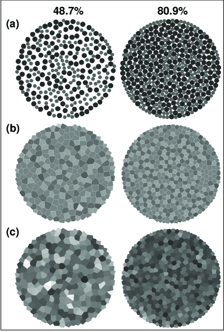
Figure 1: (a) Example configurations for area fractions $\phi=48.7\%$ and $\phi=80.9\%$, with the big beads colored darker than the small beads. (b-c) Voronoi tessellations for these configurations with cells shaded darker for increasing coordination number and circularity, respectively.

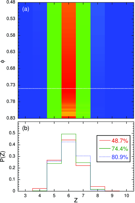
Figure 2: (Color online) (a) Contour plot of the coordination number distribution; red is for large probability density and blue is for small. The dashed white line indicates $\phi=0.74$. (b) Coordination number distributions for three area fractions, as labeled.

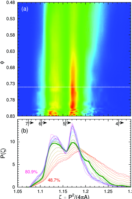
Figure 3: (Color online) (a) Contour plot of the non-circularity shape factor distributions for the Voronoi tessellation polygons. Beyond about $74\%$ (dashed white line) a well formed second peak develops and the distribution doesn’t change much. (b) Shape factor distributions for a sequence of area fractions; the thick green curve is for $\phi=74.4\%$. The labels 7, 6, 5, and 4 show the minimum shape factors for polygons with that number of sides.

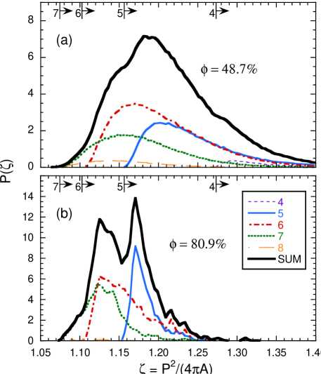
Figure 4: (Color online) Non-circularity shape factor distributions for the Voronoi tessellation polygons for (a) $\phi=48.7\%$ and (b) $\phi=80.9\%$. Thick black curves are the actual distributions, and the thin colored curves are the contributions from cells with different numbers of sides, as labeled.

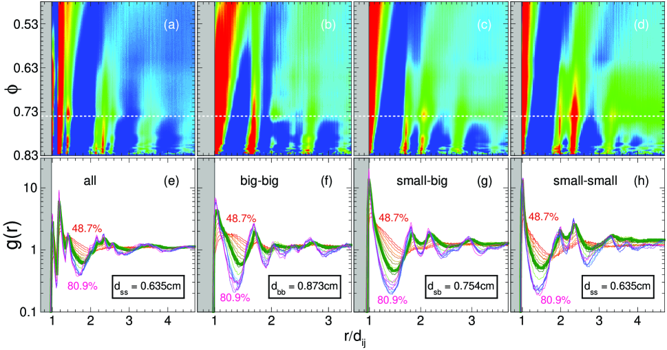
Figure 5: (Color online) The radial distribution function computed between (a,e) all beads; (b,f) big beads; (c,g) small and big beads; and (d,h) small beads. The top row shows contour plots, where blue is for large $g$ and red is for small; the dashed white line represents $\phi=0.74$. The bottom row shows data curves for different area fractions; the thick green curves are for $\phi=0.744$. The grayed region represents the distance excluded by hard-core contact, for $r$ less than the sum $d_{ij}$ of radii.

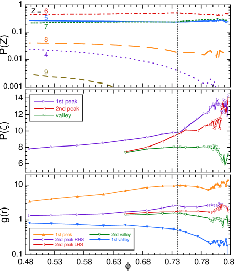
Figure 6: (Color online) The area fraction dependence of (a) the occurrence probability $P(Z)$ of Voronoi cells with $Z$ sides, and peak and valley values of (b) the shape factor distribution and (c) the pair distribution function for small beads.

III.1 Coordination number

Perhaps the simplest structural quantity is the coordination number $Z$, equal to the number of nearest neighbors for each bead. This can be most conveniently measured by constructing a Voronoi tessellation, which is dual to the position representation, and by counting the number of sides of each polygonal Voronoi cell. Examples are shown in Fig. 1b for the same configurations shown in Fig. 1a. Here the Voronoi cells are shaded darker for greater numbers of sides. The coordination number ranges between 3 and 9, but by far the most common numbers are 5, 6, and 7 irrespective of area fraction. It seems that 5- and 7-sided cells appear together, and that 6-sided cells sometimes appear in small compact clusters.

The distribution $P(Z)$ of coordination numbers, and trends vs area fraction, are displayed in Fig. 2. The results are obtained by averaging over all times and over all beads away from the boundary. The bottom plot shows actual distributions for three area fractions, two of which are the same as in Fig. 1. The main effect of increasing the area fraction is to increase the fraction of 7-sided cells at the expense of all others, until essentially only 5-6-7 sided cells remain. This trend is more clearly displayed in a contour plot, Fig. 2a, where the value of $P(Z)$ is indicated by color as a function of both $Z$ and area fraction $\phi$. For area fractions above about 74%, indicated by a dashed white line, the 4-, 8-, and 9-sided cells have essentially disappeared. This effect is rather subtle, owing to the discrete nature of the coordination number. Six-sided cells are always the most plentiful; their abundance gently peaks near 74%.

III.2 Circularity

A more dramatic measure of structural change upon approach to jamming is found by considering the shapes of the Voronoi cells. One choice for a dimensionless measure of deviation from circularity is

$$\zeta=P^{2}/(4\pi A),$$ (1)

where $P$ is the cell perimeter and $A$ is the cell area. This quantity was recently used to study crystallization of two-dimensional systems, both in simulation Moucka and Nezbeda (2005) and experiment Reis et al. (2006). By construction $\zeta$ equals one for a perfect circle, and is higher for more rough or oblong shapes; for a regular $Z$-sided polygon it is

$$\zeta_{Z}=(Z/\pi)\tan(\pi/Z),$$ (2)

which sets a lower bound for other $Z$-sided polygons. As an example in Fig. 1c the Voronoi cells are shaded darker for more circular shapes, i.e. for those with smaller non-circularity shape factors. Since $\zeta_{Z}$ decreases with increasing $Z$, it may be expected that the shape factor is related to coordination number. The advantage is that $\zeta$ is a continuous variable while $Z$ is discrete.

Shape factor distributions, $P(\zeta)$, and the way they change with increasing area fraction, are displayed in Fig. 3b. These are obtained by constructing Voronoi tessellations, and averaging over all times and over all beads. At low area fractions, $P(\zeta)$ exhibits a single broad peak. At higher area fractions, this peaks moves to lower $\zeta$, i.e. to more circular domains, and eventually bifurcates into two sharper peaks. This trend can be seen, too, in the contour plot of Fig. 3a where color indicates the value of $P(\zeta)$ as a function of both non-circularity $\zeta$ and area fraction $\phi$. This plot shows that the double peak becomes essentially completely developed around $\phi=0.74$. This is the same area fraction singled out by a subtle change in the coordination number distribution. Thus the shape factor and its distribution are useful for tracking the change in structure as a liquid-like system approaches a disordered jammed state.

The origin of the double peak in the shape factor distribution $P(\zeta)$ can be understood by considering the contributions $P_{Z}(\zeta)$ made by cells with different coordination numbers. These contributions are defined such that $P(\zeta)=\sum_{Z=3}^{\infty}P_{Z}(\zeta)$ and $P(Z)=\int_{\zeta_{Z}}^{\infty}P_{Z}(\zeta){\rm d}\zeta$; in particular, cells with coordination number $Z$ contribute a sub-distribution $P_{Z}(\zeta)$ which must vanish for $\zeta<\zeta_{Z}$ according to Eq. (2) and which subtends an area equal to the coordination number probability. As an example, the shape factor distribution is shown along with the individual contributions in Fig. 4. At low area fractions, in the top plot, the broad peak in $P(\zeta)$ is seen to be composed primarily of overlapping broad contributions from 5-, 6-, and 7-sided cells. At high area fractions, in the bottom plot, the double peak in $P(\zeta)$ is seen to be caused by 5-sided cells for the right peak and by overlapping contributions of 6- and 7-sided cells for the left peak. At these higher area fractions, the individual contributions $P_{Z}(\zeta)$ are more narrow and rise more sharply from zero for $\zeta>\zeta_{Z}$. In other words, the Voronoi cells all become more circular at higher packing fractions. Due to disorder, there is a limit to the degree of circularity that cannot be exceeded and so the changes in the circularity distribution eventually saturate. For our system this happens around $\phi=0.74$, which is well below random close packing at $\phi_{c}=0.83$.

III.3 Radial distribution

We now present one last measure of structure that is commonly used in amorphous systems: the radial or pair distribution function $g(r)$. This quantity relates to the probability of finding another bead at distance $r$ away from a given bead. For large $r$, it is normalized to approach one – indicating that the system is homogeneous at long length scales. For small $r$ in hard-sphere systems like ours, it vanishes for $r$ less than the sum of bead radii. Since we have two species of beads, big and small, there are four different distributions to consider: between any two beads, between only big beads, between big and small beads, and between only small beads.

Data for all four radial distribution functions are collected in Fig. 5. As usual, these data were obtained by averaging over all times and over all beads away from the boundary. The bottom row shows functions plotted vs $r$ for different area fractions, while the top row shows contour plots where color indicates the value of $g(r)$ as a function both $r$ and area fraction; radial distance is scaled by the sum of bead radii $d_{ij}$. All four radial distribution functions display a global peak at hard core contact, $r/d_{ij}=1$. For increasing area fractions, these peaks become higher and more narrow, while oscillations develop that extend to larger $r$. Also, near $r/d_{ij}=2$ there develops a second peak that grows and then bifurcates into two separate peaks. Both the growth of the peak at $r/d_{ij}=1$, relative to the deepest minimum, and the splitting of the peak near $r/d_{ij}=2$ have been taken as structural signatures of the glass transition Cargill (1970); Wendt and Abraham (1978); Silbert et al. (2006). For our system the split second peak becomes fully developed for area fractions greater than about $\phi=0.74$, the same area fraction noted above with regards to changes in the Voronoi tessellations.

III.4 Summary

Well-defined features develop in several structural quantities as the area fraction increases. The most subtle is an increase in the number of 7-sided Voronoi cells at the expense of all other coordination numbers, and the disappearance of nearly all 4- and 9-sized cells. The most obvious are the splitting of peaks in the shape factor distribution and the radial distribution functions. These key quantities are extracted from our full data sets and are displayed vs area fraction $\phi$ in Fig. 6. The top plot shows the fraction $P(Z)$ of Voronoi cells with $Z$ sides, for several coordination numbers; the middle plot shows peak and valley values of the probability density $P(\zeta)$ for Voronoi cells with shape factor $\zeta$; the bottom plot shows peak and valley values of the pair distribution function $g(r)$ for small beads. These three plots give a consistent picture that $\phi=0.74$ is the characteristic area fraction for structural change.

IV Dynamics

IV.1 Data

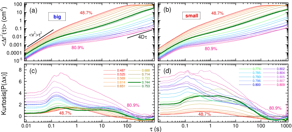
Figure 7: (Color online) (a-b) Mean-squared displacement, and (c-d) kurtosis of displacement probability distribution, all as a function of delay time. The left-hand plots are for the big beads and the right-hand plots are for the small beads. Area fraction color codes for the all plots are labeled in (c-d); the thick green curve is for $\phi=74.4\%$. Note that the mean-squared displacement saturates at the square of the sample cell radius. The squares of bead diameters are $d_{b}^{2}=0.76~{}{\rm cm}^{2}$ and $d_{s}^{2}=0.40~{}{\rm cm}^{2}$. The square of the position resolution is $(0.0016~{}{\rm cm})^{2}=3\times 10^{-6}~{}{\rm cm}^{2}$.

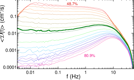
Figure 8: (Color online) Density of vibrational states of frequency $f$, for various packing fractions; the thick green curve is for $\phi=74.4\%$.

For the remainder of the paper we focus on bead motion, and how it changes in response to the structural changes found above an area fraction of $74\%$. The primary quantity we measure and analyze is the mean-squared displacement (MSD) that the beads experience over a time interval $\tau$: $\langle\Delta r^{2}(\tau)\rangle$ vs $\tau$. The MSD is readily measured directly from time- and ensemble averages of the position vs time data; it can also be computed efficiently from position autocorrelation data using Fourier methods. Results are shown in Figs. 7a-b for the big and small beads, separately. At short times, the bead motion is ballistic and characterized by a mean-squared speed according to $\langle\Delta r^{2}(\tau)\rangle=\langle v^{2}\rangle\tau^{2}$. Our frame rate is 120 Hz, corresponding to a shortest delay time of $\tau=0.0083$ s, which is fast enough that we are able to observe ballistic motion over about one decade in time for all area fractions. At long times, the bead motion is diffusive and characterized by a diffusion coefficient according to $\langle\Delta r^{2}(\tau)\rangle=4D\tau$. Our run durations are 20 minutes, corresponding to a longest delay time of $\tau=1200$ s, which are long enough for the beads to explore the entire system several times at the lowest area fractions. The crossover from ballistic to diffusive regimes becomes progressively slower as the area fraction increases. Our run durations are long enough to fully capture the diffusive regime at all but the highest area fractions. Thus our full position vs time dataset, for all beads and area fractions, should suffice for a complete and systematic study of changes in dynamics as jamming is approached.

The MSD has long been used to characterize complex dynamics. In simple systems there is a single characteristic time scale given by the crossover from ballistic to diffusive regimes. In supercooled or glassy systems, the crossover is much more gradual and there are two characteristic time scales. The shortest, called the ‘$\beta$’ relaxation time, is given by the end of the ballistic regime. The longest, called the ‘$\alpha$’ relaxation time, is given by the beginning of the diffusive regime. At greater degrees of supercooling in glass-forming liquids, and at greater packing fractions in colloidal suspensions, the $\alpha$ relaxation time increases and a corresponding plateau develops in the MSD. As seen in our MSD data of Figs. 7a-b, this same familiar sequence of changes occurs in our system as well. The greater the delay in the onset of diffusive motion, the more ‘supercooled’ is our system and the closer it is to being jammed – where each bead has a fixed set of neighbors that never changes.

Another similarity between the dynamics in our system and thermal systems can be seen by examining the kurtosis of the displacement distribution. For a given delay time, there is a distribution $P(\Delta x)$ of displacements. By symmetry the average displacement and other odd moments must all vanish. The second moment is the most important; it is the MSD already discussed. If the distribution is Gaussian, a.k.a. normal, then all other even moments can be deduced from the value of the MSD. For example the ‘kurtosis’ is the fourth moment scaled by the square of the MSD and with the Gaussian prediction subtracted; by construction it equals zero for a Gaussian distribution, and otherwise is a dimensionless measure of deviation from ‘normality’. The kurtosis of the displacement distribution has been used in computer simulation of liquids, both simple Rahman (1964) and supercooled Thirumalai and Mountain (1993); Hurley and Harrowell (1996); Kob et al. (1997), as well as in scattering Van Megen and Underwood (1988) and imaging experiments of dense colloidal suspensions Kasper et al. (1998); Marcus et al. (1999); Kegel and van Blaaderen (2000); Weeks et al. (2000). These works consider a quantity $\alpha_{2}$ equal to $1/3$ of the kurtosis, and find that the displacement distribution is Gaussian in ballistic and diffusive regimes, but becomes non-Gaussian with a peak in the kurtosis at intermediate times. We computed the kurtosis of the displacement distribution for our system, with results displayed vs delay time in Figs. 7c-d for many area fractions. As in thermal systems, our kurtosis results display a peak at intermediate times and becomes progressively more Gaussian at late times. Furthermore, the peak increases dramatically once the area fraction rises above about 74%, particularly for the large beads.

The kurtosis data in Figs. 7c-d do not vanish at short times, by contrast with thermal systems. Instead, we find that the kurtosis decreases to the left of the peak and saturates at a nonzero constant upon entering the ballistic regime. At these short times, the displacement distribution has the same shape as the velocity distribution since $\Delta x=v_{x}\tau$. Indeed our velocity distributions are non-Gaussian with the same kurtosis as the short-time displacement distributions. This reflects the non-thermal, far-from-equilibrium, driven nature of our air-fluidized system. Another difference from thermal behavior, as we’ll show in the next subsection, is that the two bead species have different average kinetic energies – which is forbidden by equipartition for a thermal systems.

While the second and fourth moments of the displacement distributions capture many aspects of bead motion, another dynamical quantity has been considered recently O’Hern et al. (2003); Silbert et al. (2005); Wyart et al. (2005a, b): the density $\langle{\cal D}(f)\rangle$ of vibrational states of frequency $f$. At high frequencies, the behavior of $\langle{\cal D}(f)\rangle$ reflects the short time ballistic nature of bead motion. At low frequencies, the behavior of $\langle{\cal D}(f)\rangle$ reflects on slow collective relaxations. If the system is unjammed, there will be zero-frequency translational relaxation modes with relative abundance set by the value of $\langle{\cal D}(0)\rangle$. If the system is fully jammed, by contrast, there can be no zero-frequency modes and hence $\langle{\cal D}(f)\rangle$ must vanishes for decreasing $f$. Thus the form and the limit of $\langle{\cal D}(f)\rangle$ at low frequencies give a sensitive dynamical signature of the approach to jamming. This shall be our focus, while by contrast in Refs. O’Hern et al. (2003); Silbert et al. (2005); Wyart et al. (2005a, b) the focus was on the behavior of low frequency modes above close packing on approach to unjamming.

The density of states may be computed from the velocity time traces, $v_{i}(t)$, for all beads $i$ Dove (1993). The mass-weighted ensemble average of time-averaged velocity autocorrelations, $w(\tau)=\sum m_{i}\langle{\bf v}_{i}(t)\cdot{\bf v}_{i}(t+\tau)\rangle/\sum m_{i}$, is the key intermediate quantity; its Fourier transform is $w(f)$ and has units of cm²/s. The final step is to compute the modulus,

$$\langle{\cal D}(f)\rangle=\sqrt{w(f)w^{*}(f)}.$$ (3)

The angle-brackets in this notation are a reminder that this is an ensemble average of single-grain quantities. By construction, the integral of Eq. (3) over all frequencies is equal to the mass-weighted mean-squared speed of the beads. While Eq. (3) appears to be a purely mathematical manipulation, the identification of the right-hand side with the density of states requires that modes be populated according to the value of $kT$; hence, for non-thermal systems like ours, the result is an effective density of states that only approximates the true density of states. Whatever the accuracy of this identification, both the expression for $\langle{\cal D}(f)\rangle$ in Eq. (3) and the mean-squared displacement may be computed from velocity autocorrelations, and thus do not embody different physics; rather, they give complementary ways of looking at the same phenomena and serve to emphasize different features.

The effective density of vibrational states for our system of air-fluidized beads is shown in Fig. 8, with separate curves for different area fractions. At low $\phi$ there are many low frequency modes and $\langle{\cal D}(f)\rangle$ is nearly constant until dropping off at high frequencies. At higher $\phi$, the number of low frequency modes gradually decreases; $\langle{\cal D}(f)\rangle$ is still constant at low $f$, but it increases to a peak before dropping off at high $f$. Even at the highest area fractions, $\langle{\cal D}(f)\rangle$ is nonzero at the smallest frequencies observed, as given by the reciprocal of the run duration.

IV.2 Short and long-time dynamics

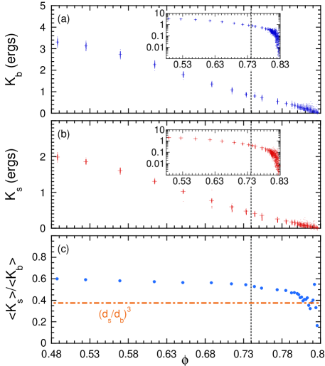
Figure 9: (Color online) (a-b) Kinetic energy vs area fraction for big and small beads, respectively. The time-average for each bead is shown by a small dot; the ensemble average over all beads is shown by $+$. (c) The kinetic energy ratio of small-to-big beads. The line $(d_{s}/d_{b})^{3}$ shows where beads move with the same mean-squared velocity. Insets show the same quantities on a logarithmic scale.

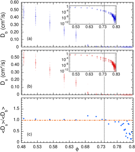
Figure 10: (Color online) (a-b) Diffusion coefficient vs area fraction for big and small beads, respectively. The time-average for each bead is shown by a small dot; the ensemble average over all beads is shown by $+$. (c) The diffusion coefficient ratio of small-to-big beads. Insets show the same quantities on a logarithmic scale.

The quantities that specify the ballistic and diffusive motion at short and long times, respectively, are the mean-squared speeds and the diffusion coefficients. These may be deduced from the mean-squared displacement data, separately for each bead. We now examine trends in these dynamical quantities as a function of area fraction.

We begin with the mean-squared speed. To highlight the contrast with a thermal system, we convert it to a mean kinetic energy and plot the results in Figs. 9a-b for the big and small beads, respectively. We show a small point for each individual bead, as well as a larger symbol for the ensemble average of these values. The average kinetic energies appear to decrease nearly linearly towards zero as the area fraction is raised towards random close packing. The scatter in the points is roughly constant, independent of $\phi$, and reflects the statistical uncertainty in our velocity measurements. There is no evidence of nonergodicity or inhomogeneity in energy injection by our air-fluidization apparatus; namely, all the beads of a given species have the same average kinetic energy to within measurement uncertainty. Beyond about $\phi=0.81$ the uncertainty becomes comparable to the mean, as set by our speed resolution, and we can no longer readily discern the average kinetic energies. This may be more evident in the insets, which show kinetic energies on a logarithmic scale.

Note that the big and small beads have different average kinetic energies. Equipartition is thus violated for our athermal, driven system. This is highlighted in Fig. 9c, which shows the kinetic energy ratio of small to large beads. This ratio is roughly constant at about 0.6 for the lowest area fractions. It decreases gradually for increasing $\phi$, at first gradually and then more rapidly beyond about $\phi=0.78$. There is no obvious feature at $\phi=0.74$, where structural quantities changed noticeably. Interestingly, however, the kinetic energy ratio appears to head toward the cube of the bead diameter ratio on approach to random close packing. This means that the mean-squared speeds are approaching the same value, perhaps indicating that only extremely collective motion is possible very close to jamming. In order for one bead to move, the neighboring bead in the path of motion must move with the same speed. This seems a natural geometrical consequence of nearly close packing, but would be a violation of equipartition in a thermal system.

Turning now to late-time behavior, we display diffusion coefficients vs area fraction in Figs. 10a-b, for big and small beads respectively. As in Fig. 9, a small dot is shown for each individual bead and a larger symbol is shown for the ensemble average of these results. The average diffusion coefficients appear to decrease linearly with increasing area fraction, starting at the lowest $\phi$. Here there is considerable scatter in the data, reflecting a level of uncertainty set by run duration. Linear fits of diffusion coefficient vs area fraction in this regime extrapolate to zero at the special value $\phi=0.74$. However, just before reaching this area fraction, the data fall below the fit. As shown on a logarithmic scale in the insets, the diffusion coefficients are nonzero and continue to decrease with increasing $\phi$. Beyond about $\phi=0.81$ the system becomes non-ergodic over the duration of our measurements. Namely, some beads remain stuck in the same nearest neighbor configurations while others have broken out. Indeed, at these high area fractions the MSDs in Fig. 7 grow sublinearly at the latest observed times. To obtain reliable diffusion coefficient data in this regime would require vastly longer run durations.

IV.3 Timescales

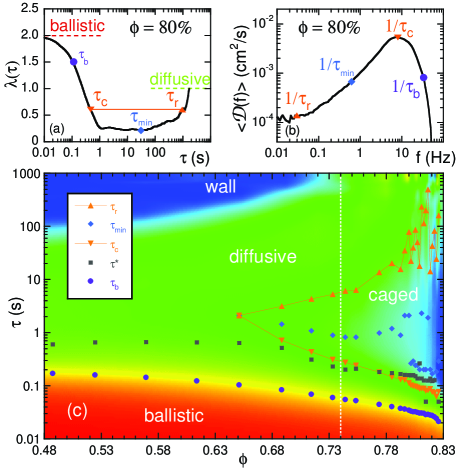
Figure 11: (Color online) (a) Logarithmic derivative $\lambda$ of the mean-squared displacement vs delay time, for big beads at area fraction $\phi=80\%$. Four special time scales can be defined from such data, as depicted: $\tau_{b}$ where $\lambda=1.5$, $\tau_{\rm min}$ where $\lambda$ is minimum, and $\tau_{c}$ and $\tau_{r}$ where $\lambda$ is halfway between 1 and its minimum. (b) Density of state, for big beads at $\phi=80\%$, marked with the four special timescales. (c) Contour plot of the logarithmic derivative for the big beads, where color indicates the value of $\lambda$, as a function of both area fraction and delay time. Red is slope two and blue is slope zero; caged dynamics are when the mean-squared displacement has a slope less than one, which is aqua-blue. The four special times defined by the behavior of $\lambda$, as well as a fifth time $\tau^{*}$ at which the displacement kurtosis is maximal, are superposed on the contour plot; symbol key is given in the legend.

Lastly we focus on characterizing several special times that serve to demarcate the short-time ballistic and the long-time diffusive regimes seen in the displacement statistics data. The time scale-dependent nature of the dynamics, which is obvious in the MSD or the density of states, is also obvious in real-time observations or in AVI movie data. For high area fractions, the bead configuration appears immutable at first; the beads collide repeatedly with an apparently-fixed set of neighbors that cage them in. Only with patience, after hundreds or thousands of collisions, can the beads be observed to break out of their cages, change neighbors, and begin to diffuse throughout the system.

To measure unambiguously the characteristic timescales, we consider the slope of the mean-squared displacement as seen on a log-log plot:

$$\lambda(\tau)={\partial\ln[\langle\Delta r^{2}(\tau)\rangle]\over\partial\ln\tau}.$$ (4)

An example for one of the higher area fractions is shown in Fig. 11a. At the shortest delay times, when the motion is perfectly ballistic, this slope is 2; at the longest delay times, when the motion is perfectly diffusive, this slope is 1. For high area fractions, such as shown, there is a subdiffusive regime with $\lambda<1$ at intermediate times; this is when a typical bead appears by eye to be stuck in a cage, rattling against a fixed set of neighbors. For low area fractions, not shown, there is no such ‘caging’ and $\lambda$ decreases monotonically from 2 to 1.

Several natural time scales can now be defined with use of $\lambda(\tau)$ vs $\tau$ data. The shortest is the delay time $\tau_{b}$ at which the logarithmic slope falls to $\lambda(\tau_{b})=1.5$. This demarcates the ballistic regime, below which the bead velocity is essentially constant. At high area fractions, $\tau_{b}$ is a typical mean-free time between successive collisions; at low area fractions, $\tau_{b}$ it is also the time for crossover to diffusive motion. The other time scales that we define all refer to the subdiffusive, caging dynamics at high area fractions. The most obvious is the delay time $\tau_{\rm min}$ at which $\lambda(\tau_{\rm min})$ is minimum; this corresponds to an inflection in the MSD on a log-log plot. Below $\tau_{\rm min}$ most beads remain within a fixed cage of neighbors. The last two special times specify the interval when the motion is subdiffusive, with a logarithmic slope falling in the range below 1 and above its minimum. The smaller is the delay time $\tau_{c}$ at which the logarithmic slope decreases half-way from 1 down towards its minimum: $\lambda(\tau_{c})=[1+\lambda(\tau_{\rm min})]/2$. This is the time at which the beads have explored enough of their immediate environment to ‘realize’ they are trapped at least temporarily within a fixed cage of neighbors; it is longer, and distinct from, the mean-free collision time. The longest special time scale is the delay time $\tau_{r}$ at which the logarithmic slope increases half-way from its minimum up towards 1: $\lambda(\tau_{r})=[1+\lambda(\tau_{\rm min})]/2$. This is the time beyond which the beads rearrange and break out of their cages; it demarcates the onset of fully diffusive motion.

Before continuing, we note that these four special times also correspond to features in the density of states. As shown in Fig. 11b, the density of states drops to zero precipitously for frequencies above $1/\tau_{b}$, the reciprocal of the ballistic- or collision mean-free time. The density of states reaches a peak at $1/\tau_{c}$, corresponding to the time that beads ‘realize’ they are stuck at least temporarily within a cage. For lower frequencies, the logarithmic derivative of $\langle{\cal D}(f)\rangle$ vs $f$ has an inflection at roughly $1/\tau_{\rm min}$. And at the lowest frequencies, $\langle{\cal D}(f)\rangle$ approaches a constant value below about $1/\tau_{r}$. Thus we could have analyzed all data in terms of $\langle{\cal D}(f)\rangle$; however we prefer to work with the mean-squared displacement since it does not involve numerical differentiation.

Results for the special timescales are collected in Fig. 11 as a function of area fraction. Actual data points are superposed on top of a contour plot of the logarithmic derivative, where color [on-line] fans through the rainbow according to the value of $\lambda$: red for ballistic, green for diffusive, and blue for subdiffusive. With increasing $\phi$, the ballistic time scale decreases steadily by a factor of nearly ten as close as we can approach random close packing. Note that with our definition of $\tau_{b}$, these data points lie near the center of the yellow band demarcating the end of the red ballistic regime. Below $\phi=0.65$ the motion is never subdiffusive, and $\tau_{b}$ is the only important time scale. Right at $\phi=0.65$ the motion is only barely subdiffusive, for a brief moment, so that all three associated times scales nearly coincide. Above $\phi=0.74$ the caging is sufficiently strong that the time scale for rearrangement $\tau_{r}$ is ten times longer than the time scale $\tau_{c}$ for ‘realization’ that there is caging. At progressively higher area fractions this separation in time scales grows ever stronger. On approach to jamming at random close packing, the cage realization time decreases towards a nonzero constant, while the cage break-up or rearrangement time $\tau_{r}$ increases rapidly towards our run duration and appears to be diverging.

Note that the two time scales $\tau_{c}$ and $\tau_{r}$ capture the subdiffusive caging dynamics better than just the delay time $\tau_{\rm min}$ at which the logarithmic derivative is minimum and the motion is maximally subdiffusive. One reason is that $\tau_{\rm min}$ is difficult to locate for extremely subdiffusive motion, where there is a wide plateau in the MSD and hence where $\lambda$ is nearly zero over a wide range of delay times. This difficulty can be seen in both Fig. 11a, where $\lambda$ remains close to its minimum for over two decades in delay time, as well as in Fig. 11c above about $\phi=0.8$, where $\tau_{\rm min}$ data jump randomly between about 2 s and about $3\tau_{c}$. The other reason is that $\tau_{\rm min}$ does not appear to be either a linear or geometric average of the cage ‘realization’ and breakup times. Rather, the shape of $\lambda(\tau)$ vs $\ln(\tau)$ is asymmetric, with a minimum closer to the cage ‘realization’ time. Thus it is useful to know the two times $\tau_{c}$ and $\tau_{r}$ that together specify the subdiffusive dip of $\lambda(\tau)$ below one, just as it is useful to know the full-width half-max of a spectrum of unspecified shape.

Note too that $\tau_{c}$ and $\tau_{r}$ are distinct from the time $\tau^{*}$ at which the kurtosis is at maximum. Results for $\tau^{*}$ are extracted from our kurtosis data, and are displayed as open squares along with other characteristic times in Fig. 11. At low area fractions, even when there is no subdiffusive regime, the kurtosis exhibits a maximum at delay time $\tau^{*}$ that is several times the ballistic / collision time $\tau_{b}$. With increasing area fraction, $\tau^{*}$ decreases. Once a subdiffusive regime appears, the value of $\tau^{*}$ is close to the time $\tau_{c}$ at which grains ‘realize’ they are stuck in a cage. Data in Fig. 11 for both $\tau_{c}$ and $\tau^{*}$ decrease with increasing area fraction, $\phi$, on approach to jamming, while the time $\tau_{r}$ signalling the end of the subdiffusive regime appears to grow without bound. The decrease of $\tau^{*}$ with $\phi$ agrees with previous observations on colloids Marcus et al. (1999); Kegel and van Blaaderen (2000); Weeks et al. (2000), but contrasts with statements that $\tau^{*}$ corresponds to the cage-breakout $\alpha$-relaxation time beyond which the motion is diffusive. To emphasize, we find that the tail of the displacement distribution is largest relative to a Gaussian, and hence that the kurstosis is maximal, at the beginning of the subdiffusive regime. At that time most beads have been turned back by collision, but a few prolific beads move at ballistic speed roughly one diameter – which is long compared to the rms displacement. This observation is not an artifact of limited spatial or temporal resolution or of limited packing fraction range, which are all notably better than in previous experiments. It is also not an artifact of our analysis method; indeed, if we filter too strongly then the kurtosis peak shifts to later times.

IV.4 Jamming phase diagram

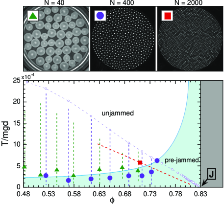
Figure 12: (Color online) The zero-stress plane of the jamming phase diagram showing our trajectories in phase space. The primary trajectory, which corresponds to sequences shown in all previous plots, is given by the diagonal dashed purple curve and open circles that intersects the “pre-jammed” boundary at $74\%$ and that ends at Point J, $\{\phi\approx 0.83,T=0\}$. The grayed region is forbidden for impenetrable beads. The solid circles, triangles, and square denote measurements of the phase boundary for large hollow polypropylene beads, solid steel beads, and tiny solid steel beads, as shown in the images. Each boundary point corresponds to the trajectory indicated by the dashed going through it.

Before closing we now summarize our structure and dynamics observations and place them in the context of the jamming phase diagram. By adding more beads to our system at fixed air speed, we control the approach to jamming two ways. First, most obviously, the area fraction increases towards random close packing at $\phi_{c}=0.83$. Second, the average kinetic energy of the beads decreases – roughly linearly with $\phi$ according to the kinetic energy data shown in Fig. 9. Both aspects are captured by the trajectory on a jamming phase diagram plot of kinetic energy vs area fraction. To get a single dimensionless measure of kinetic energy, we divide the mass-weighted average kinetic energy of the beads by a characteristic gravitational energy given by average ball weight times diameter; the result is denoted as a scaled effective temperature $T/(mgd)$. This scaling reflects the natural energy for air-mediated interactions in a gas-fluidized system. The particular $T/(mgd)$ vs $\phi$ trajectory followed by our experiments is shown by open symbols in Fig. 12. It is a diagonal line that terminates at $\{T=0,\ \phi=\phi_{c}\}$, which is the special point in the jamming phase diagram known as ‘Point-$J$’ O’Hern et al. (2002, 2003). On approach to Point-$J$ our system remains unjammed, but develops tell-tale features in the Voronoi tessellations and in the mean-squared displacement indicating that jamming is near. In particular the structural changes saturate, and the ratio $\tau_{r}/\tau_{c}$ of cage breakup to ‘realization’ times exceeds ten, for points along the trajectory closer to Point-$J$ than $\{T/(mgd)=0.007,\phi=0.74\}$; we then say the system is ‘pre-jammed’. In this pre-jammed region, we did not observe any signs of aging; the structure and dynamics change from that of a simple liquid but do not appear to evolve with time.

An extended region of ‘pre-jammed’ behavior must exist near Point-$J$, and can be mapped out by changing the experimental conditions. The simplest variation is to examine vertical trajectories, at fixed $\phi$ for the same system of steel beads, where the effective temperature is changed by the speed of the upflowing air. We did this for several different area fractions, locating the special effective temperatures below which the system becomes pre-jammed. Furthermore, to better test the universality of our phase diagram and the choice of energy scaling, we examined two other 1:1 bidisperse mixtures of spheres. This includes several constant-$\phi$ trajectories for large hollow polypropylene spheres with diameters of 1-1/8 and 1-3/8 inches, and one constant air speed trajectory for very small steel spheres with diameters of 5/32 and 1/8 inches. The resulting trajectories and pre-jamming boundary points are shown in Fig. 12 as dashed lines and symbols, respectively. In spite of the vast differences in bead systems, a remarkably consistent region of pre-jammed behavior appears in the temperature vs area fraction jamming phase diagram.

V Conclusion

The quasi-2D system of air-fluidized beads studied in this paper is fundamentally different from an equilibrium system. Here all microscopic motion arises from external driving, and has nothing to do with thermodynamics and ambient temperature. Rather there is a constant input of energy from the fluidizing air, and this excites all motion. As a result of thus being far from equilibrium, the velocity distributions are not Gaussian. Furthermore, the average kinetic energy of the two species is not equal because of how they interact with the upflow of air.

In spite of these differences, our system exhibits hallmark features upon approach to jamming that are very similar to the behavior of thermal systems. In terms of structure, our system develops a split peak in the circular factor distribution and a split second peak in the pair distribution function. In terms of dynamics, our system develops a plateau in the mean-squared displacement at intermediate times, between ballistic and diffusive regimes, where the beads are essentially trapped in a cage of nearest neighbors. And also like a thermal system, the prominence of these features increases with both increasing packing fraction and with decreasing particle energy, in a way that can be summarized by a jamming phase diagram.

The significance of the above conclusions is to help reinforce the universality of the jamming concept beyond just different types of thermal systems, to a broader class of non-equilibrium systems as well. This suggests that the geometrical constraints of disordered packing plays the major role. Our system of air-fluidized beads may now serve as a readily-measured model in which to study further aspects of jamming that are not readily accessible in thermal systems. For example it should now be possible to characterize spatial heterogeneities and dynamical correlations in our system, expecting the results to shed light on all systems, thermal or not, that are similarly close to being jammed.