Signatures of the superfluid to Mott-insulator transition in the excitation spectrum of ultracold atoms

Abstract

We present a detailed analysis of the dynamical response of ultra-cold bosonic atoms in a one-dimensional optical lattice subjected to a periodic modulation of the lattice depth. Following the experimental realization by Stöferle et al [Phys. Rev. Lett. 92, 130403 (2004)] we study the excitation spectrum of the system as revealed by the response of the total energy as a function of the modulation frequency $\Omega$. By using the Time Evolving Block Decimation algorithm, we are able to simulate one-dimensional systems comparable in size to those in the experiment, with harmonic trapping and across many lattice depths ranging from the Mott-insulator to the superfluid regime. Our results produce many of the features seen in the experiment, namely a broad response in the superfluid regime, and narrow discrete resonances in the Mott-insulator regime. We identify several signatures of the superfluid-Mott insulator transition that are manifested in the spectrum as it evolves from one limit to the other.

1 Introduction

The realization of ultracold atoms confined in optical lattices has made a large range of fundamental equilibrium and dynamical phenomena of degenerate quantum gases experimentally accessible. The success of this approach stems from the fact that, in contrast to analogous condensed matter systems, optical lattices form a defect free lattice potential which can trap a dense cloud of atoms with long decoherence times and can be controlled rapidly with a great deal of flexibility. This has already enabled a seminal demonstration of the superfluid (SF) to Mott insulator (MI) transition by Greiner et al [1] that was predicted to occur for a clean realization of the Bose-Hubbard model (BHM) [2, 3]. More recently, other themes of ultracold-atom research have been explored experimentally such as the purely one-dimensional (1D) Tonks-Girardeau limit [4, 5], the characterization of the SF-MI transition via the excitation spectrum through 1D - 3D dimensionality crossover [6, 7], and impurity effects caused by Bose-Fermi mixtures [8, 9].

Here we focus on features of the excitation spectrum from reference [6] which were revealed for a 1D BHM by periodic modulation of the lattice depth. The experimental accessibility of the excitation spectrum provides a rich source of additional information that can be compared with well studied quantities such as the dynamic structure factor [10, 11]. In addition to this the experiment demonstrates the transition through the evolution of the spectrum from discrete sharp resonances in the MI regime to a broad continuum of excitations in the SF regime. Changes in the structure of the excitation spectrum provide important evidence for the transition beyond the loss and revival of phase coherence when ramping the lattice [1], and can also be used to diagnose the temperature of the system [12, 13]. The 1D system is of particular interest for several reasons. Firstly, quantum fluctuations are expected to play a strong role there [14], and this is indeed found to be the case with the critical ratio of the on-site interaction to kinetic energy $(U/J)_{c}$, identified by the appearance of the discrete structure in the spectrum, being lower than that predicted by mean field theory [6]. Secondly, the behavior found in the 1D experiment for the SF regime, specifically a large and broad non-zero response, most strikingly departs from standard theoretical predictions. Specifically, linear response using Bogoliubov theory for a Bose-Einstein condensate (BEC) in a shallow 1D optical lattice predicts that lattice modulation cannot excite the gas in the SF regime due to the phonon nature of the excitation spectrum [15]. Since the quantum depletion of the SF in the experiment was significant ($\approx 50$%), it has been suggested that this was responsible for the response [16]. Indeed, it has been shown that only a small amount of seed depletion is required for non-linear effects like the parametric amplification of Bogoliubov modes to reproduce the SF response [17, 18]. More recently still, the use of the sine-Gordon model and bosonization method has demonstrated that linear response is non-zero at low frequencies [19]. Lastly, the study of the 1D system permits the use of quasi-exact numerical methods, such as the Time Evolving Block Decimation (TEBD) algorithm, where the fully time-dependent dynamical evolution of the system can be computed efficiently for systems of equivalent size to those in the experiment.

In addition to the many-body physics perspective, understanding the excitation spectrum revealed in [6] is important for potential applications of the MI state. The zero particle number fluctuations for an ideal commensurate MI state make them attractive candidates for several applications, most notably as a quantum memory, a basis for quantum computing [20, 21, 22, 23, 24, 25], and quantum simulations of many-body quantum systems [26, 27]. A well understood excitation spectrum can give valuable information about the nature and stability of the experimental approximation of the ideal MI state to external perturbations.

In this paper we study the dynamics of the 1D BHM under lattice modulation and generate excitation spectra for box and harmonic trapping of a large system over numerous lattice depths ranging from the SF to MI regime. We find that much of the features of the box system can be understood from a small exact calculation. However, the large system calculations were crucial for the investigation of signatures in the spectrum which indicate the transition from MI to SF regime in both trappings. We find that for a harmonically trapped system with less than unit filling the spectrum is similar to the commensurately filled box, but with the transition producing less pronounced signatures. Additional calculations progressing from the MI regime for a harmonically trapped system with a central filling greater than unity produces a spectra that has very good qualitatively agreement with the experiment. In this way our results are different but complementary to a very recent study of the same experiment by Kollath et al [28] where they discovered that excitation spectra can reveal information about the commensurateness of the system.

The structure of the paper is as follows: we give an overview of the physical setup for the 1D system in section 2.1 followed by a description of the excitation scheme in section 2.2. We then introduce the linear response formalism for this scheme in section 3.1, and in section 3.2 we give an overview of the literature describing the TEBD simulation method used here for the larger systems. The results are then presented in section 4, firstly for a small box system computed exactly in section 4.1, then for larger systems computed with the TEBD algorithm for box and harmonic trapping in section 4.2 and 4.3 respectively. We then end with the conclusions in section 5.

2 Probing the system

2.1 Optical lattices and the Bose-Hubbard model

In the experiment [6] effective 1D systems were formed from an anisotropic 3D optical lattice loaded with ultra-cold bosonic atoms [3]. This is done by adiabatically exposing a BEC to far-off resonance standing wave laser fields in three orthogonal directions forming a 3D optical lattice potential $V_{OL}({\bf r})=\sum_{d=1}^{3}V_{d0}\sin^{2}(q_{B}r_{d})$ where $q_{B}=2\pi/\lambda$ and $\lambda$ is the wavelength of the laser light yielding a lattice period $a=\lambda/2$ [29]. The height of the potential $V_{d0}$ is proportional to the intensity of the $d$-th pair of laser beams, and is conveniently expressed in terms of the recoil energy $E_{r}=q_{B}^{2}/2m$ for atoms of mass $m$ (taking $\hbar=1$ throughout).

Effective 1D systems are then formed by making laser intensities in two of the directions $r_{2}\equiv y$ and $r_{3}\equiv z$ very large ($V_{\perp}\approx 30E_{r}$). The confinement is then sufficiently strong to inhibit any tunnelling or excitations in those directions on the energy scales we are concerned with. The result is an array of many isolated effective 1D systems in the $r_{1}\equiv x$ direction  [6, 30, 4, 5]. For the remaining lattice intensity $V_{10}\equiv V_{0}$ we consider much shallower depths, but always remain deep enough ($V_{0}>4E_{r}$) to ensure that there is an appreciable band-gap between the lowest and first excited Bloch band, given in the harmonic approximation by $\omega_{ho}=2E_{r}\sqrt{V_{0}/E_{r}}$. Combined with the ultra-low temperatures of the atoms this is sufficient to ensure that the dynamics can be described by the lowest Bloch band of the lattice, and that the tight-binding approximation is applicable [3].

With the centre of lattice site $j$ in one such 1D system given by $x_{j}=ja$ we can construct a complete and orthonormal set of localized mode functions $\phi_{j}({\bf r})=w(x-x_{j})W(y)W(z)$ factorized as the product of Wannier functions $w$ and $W$ of the lowest Bloch band for the shallow and deeply confined directions respectively. After expanding the bosonic field operator $\hat{\psi}\left({\bf r}\right)$ into these modes and restricting our consideration to one 1D system, the resulting Hamiltonian $H$ reduces to the 1D BHM [3] composed of $M$ sites

$$H=-J\sum_{j=1}^{M-1}(b_{j}^{\dagger}b_{j+1}+{\rm h.c.})+\sum_{j=1}^{M}v_{j}b_{j}^{\dagger}b_{j}+\frac{U}{2}\sum_{j=1}^{M}b_{j}^{\dagger}b_{j}^{\dagger}b_{j}b_{j},$$ (1)

where the operators $b_{j}$ ($b_{j}^{\dagger}$) are bosonic destruction (creation) operators for an atom in site $j$. The parameters of the BHM are functions of the lattice depth $V_{0}$ with the matrix elements for hopping between adjacent sites $j$ and $j+1$ and on-site interaction strength given by [31]

$$J = -\int dx~{}w(x-x_{j})\bigg{(}-\frac{\hbar^{2}}{2m}\frac{d^{2}}{dx^{2}}+V_{0}\sin^{2}(q_{B}x)\bigg{)}w(x-x_{j+1}),$$

$$U = 2a_{s}\omega_{ho}\int dx~{}|w(x-x_{j})|^{4},$$ (2)

where $a_{s}$ is the $s$-wave scattering length, and a Gaussian ansatz has been used for the tightly confined Wannier states $W$. The trapping offset is well approximated as $v_{j}\approx V_{T}(x_{j},y,z)$, where $V_{T}({\bf r})$ describes an additional slowly varying trapping potential which could be due to magnetic trapping. In the case of [6] the axial potential of the 1D system was dominated by the Gaussian beam envelopes (with $1/e^{2}$ waists $l$) of the lasers for the strongly confined directions characterized by the trapping frequency $\omega_{T}=2E_{r}\frac{\lambda}{\pi l}\sqrt{V_{\perp}/E_{r}}$ [30].

The physics of the BHM is governed by the ratio $U/J$. Competition between these two terms results in a transition at temperature $T=0$ for a critical ratio $(U/J)_{c}$ from the SF to the MI regime [2, 32]. Mean-field theory for an infinite unit commensurately filled 1D system predicts that $(U/J)_{c}\approx 2\times 5.8$. However, if the strong quantum fluctuations present in 1D are taken into account, the appearance of the SF regime is not predicted to occur until the critical ratio drops to $(U/J)_{c}\approx 3.85$ [33]. The presence of trapping and the finite size of a system modifies the nature of the transition, prohibiting it from being sharp and so in line with the experiment [6] we expect the transition to occur gradually somewhere in between these limits [34].

2.2 Lattice modulation excitation scheme

In the experiment [6] the 1D system was initially prepared in the groundstate for some depth $V_{0}$, ranging from the SF to MI regime. The axial lattice depth was then subjected to a modulation of the form

$$V_{OL}(x,t)=V_{0}[1+A\sin(\Omega t)]\sin^{2}(q_{B}x),$$ (3)

where $A$ is the modulation amplitude as a fraction of the initial lattice depth, and $\Omega$ is the modulation frequency [6]. The modulation was applied for a fixed time $\tau=30$ ms after which the energy deposited into the system was measured by time-of-flight imaging of central momentum width averaged over the many 1D systems realized. The applied modulation frequency was taken to a maximum of $\Omega/2\pi=6$ kHz which defines the relevant energy scale for the system and was well below the band-gap.

To compare with the experiment we take the wavelength of the light used to form the optical lattice as $\lambda=826$ nm, and the atomic species trapped as ⁸⁷Rb, where $a_{s}=5.1$ nm, in all numerical values quoted. For our calculations we initially computed the groundstate of the system over depths $U/J=5,6,\dots,20$ for the large systems and slightly shallower depths $U/J=2,3,\dots,20$ for the small system [35], all with fixed particle number $N$. We study a small and large system with box boundaries which are commensurately filled as $M=N=7$ and $M=N=41$ respectively. We also consider a harmonically trapped system where $v_{j}=m\omega_{T}^{2}x_{j}^{2}/2$ for a slightly smaller system with $M=25$ using $\omega_{T}/2\pi=70$ Hz and $N=15$, as well as $\omega_{T}/2\pi=100$ Hz and $N=30$. These trapping frequencies are close to that in the experiment [6, 30] where $\omega_{T}/2\pi\approx 85$ Hz, and where sufficient to eliminate any occupation at the box boundaries of the system. The modulation given in equation (3) was then applied to the system by computing time-dependent BHM parameters via equation (2). This includes an implicit assumption that the Wannier states describing atoms in the lattice adiabatically follow the variations in the lattice potential induced by the modulation. Given that the timescale of atomic motion in a lattice site is $\nu=\omega_{ho}/2\pi$ and that this is typically an order of magnitude greater than the modulation frequencies applied, the adiabatic assumption is reasonable. The response of the system was then measured via the total energy $\langle H_{0}\rangle$, with respects to the unperturbed BHM, for different $\Omega$. To demonstrate the evolution of the spectra at different depths we use the same fixed range for $\Omega/2\pi$ at all depths. This range is identical to the experiment and is likewise quoted in kHz while the energy absorbed is expressed in units of $E_{r}$.

3 Analysis

3.1 Linear response

We consider a straightforward linear response treatment of this excitation scheme which follows under the same assumption used for the numerical calculation that the system is described by the BHM with time-varying parameters $J[V_{OL}(t)]$ and $U[V_{OL}(t)]$. For perturbative calculations we make an additional assumption that the modulations are weak and approximate the variation of these functions about the initial depth $V_{0}$ linearly resulting in a harmonic perturbation [19]

$$H(t)=H_{0}+AV_{0}\sin(\Omega t)\left(\delta UH_{0}-J_{0}\{\delta J-\delta U\}H_{J}\right),$$ (4)

where $H_{0}=-J_{0}H_{J}+U_{0}H_{U}$, $\delta U=\frac{d\ln U}{dV}|_{V_{0}}$, $\delta J=\frac{d\ln J}{dV}|_{V_{0}}$, $U_{0}=U[V_{0}]$ and $J_{0}=J[V_{0}]$. The perturbation is split into a part that is proportional to the unperturbed BHM Hamiltonian $H_{0}$ and a part proportional to the hopping operator $H_{J}=\sum_{j=1}^{M-1}(b_{j}^{\dagger}b_{j+1}+{\rm h.c.})$ under the proviso that $U_{0}>J_{0}$. The first part cannot induce excitations and instead gives a small time-dependent shift to the unperturbed energies which can be ignored. As a result the excitation operator of this perturbation is just the hopping operator [19, 13] with coupling $\kappa=AV_{0}J_{0}(\delta J-\delta U)$. By acting over the whole system uniformly it creates excitations with zero quasimomentum as expected.

Let us label the eigenstates of the unperturbed BHM $H_{0}$ as $\left|\,n\right\rangle$ with energy $\epsilon_{n}$. The principle quantities of interest are the excitation probabilities $P_{0\rightarrow n}(\tau,\Omega)$ for the transitions to the excited states $\left|\,n\right\rangle$ from the groundstate $\left|\,0\right\rangle$ due to this perturbation being applied for a time $\tau$ with a frequency $\Omega$. In first-order time-dependent perturbation theory these are given by

$$P^{(1)}_{0\rightarrow n}(\tau,\Omega)=\left|t^{(1)}_{0\rightarrow n}\right|^{2}=\kappa^{2}\left|\left\langle n\left|H_{J}\right|0\right\rangle I^{(1)}_{n}(\tau,\Omega)\right|^{2},$$ (5)

where $I^{(1)}_{n}(\tau,\Omega)=\int_{0}^{\tau}dt~{}e^{i\omega_{n0}t}\sin(\Omega t)$ and $\omega_{n0}=(\epsilon_{n}-\epsilon_{0})$. This result reduces under the rotating wave approximation and the limit $\tau\rightarrow\infty$ to the familiar Golden rule result. We also make use of the second-order result

$$P^{(2)}_{0\rightarrow n}(\tau,\Omega)=\left|t^{(1)}_{0\rightarrow n}-\kappa^{2}\sum_{m}\left\langle n\left|H_{J}\right|m\right\rangle\left\langle m\left|H_{J}\right|0\right\rangle I^{(2)}_{nm}(\tau,\Omega)\right|^{2},$$ (6)

where $I^{(2)}_{nm}(\tau,\Omega)=\int_{0}^{\tau}dt~{}\int_{0}^{t}dt^{\prime}~{}e^{i\omega_{nm}t}e^{i\omega_{m0}t^{\prime}}\sin(\Omega t)\sin(\Omega t^{\prime})$. The total energy absorbed by the system, relative to $H_{0}$, is then $E(\tau,\Omega)=\sum_{n}\epsilon_{n}P_{0\rightarrow n}(\tau,\Omega)-\epsilon_{0}$.

3.2 Numerical method

For the large systems investigated later in sections 4.2 and 4.3 exact integration of the many-body Schrödinger equation is not feasible. To compute these results we employed the TEBD algorithm [36, 37] which is a quasi-exact numerical method that allows the dynamical evolution of 1D quantum lattice systems with nearest-neighbor interactions to be computed efficiently and accurately. The algorithm has been successfully applied to numerous physical systems including the BHM [38, 39, 40, 41, 28, 42]. Not long after being proposed by Vidal it was recognized [39, 43] that TEBD shares some conceptual and formal similarities with the well established density matrix renormalization group (DMRG) [44, 45] method enabling the development of a new adaptive time-dependent-DMRG algorithm which incorporates optimizations from both. A detailed analysis of the accuracy and error propagation of this method was given by Gobert et al [41] and applies quite generally to TEBD also. We do not describe the TEBD algorithm here, except to mention some specific issues, and instead refer the reader to the relevant articles above for more details.

The objective of the simulations in this paper were to map out the response of the system with the modulation frequency $\Omega$ and depths $U/J$ which cross the SF-MI transition. For sufficient sampling this required in excess of 1000 simulations for both the box and harmonically trapped systems presented here. Consequently we were limited for practical reasons to using a truncation parameter $\chi=30$ (see [37] for an explanation of $\chi$) for all simulations which was lower than that strictly necessary in order to achieve full convergence. Thus we cannot claim that our calculations are quasi-exact and would not expect the many-body state given by the simulation at the end to have a high fidelity with the true state of the system. Instead we treat our calculation as an approximation in the same spirit as the Gutzwiller ansatz [2, 46] (where $\chi=1$), but with the important difference that since $\chi>1$ we are permitting a non-negligible amount of quantum correlations. Given that we are only interested in the total energy, which is an observable composed of one- and two-particle correlations, we expect that this approximation should yield quantitative agreement for the system sizes and regimes considered here. Indeed, we have carried out more accurate calculations at specific points which reveal that the total energy is a robust observable with respects to truncation [47]. Consequently, the features of the energy spectrum do emerge, even with this relatively low $\chi$, and the approximations made do not invalidate the results presented here. For simulations of the lattice modulation problem at some specific lattice depths with larger $\chi$ see the recent work by Kollath et al [28].

4 Results

4.1 Exact calculation for a small system

We begin by studying the exact dynamical evolution of the BHM under the lattice modulation for a small system composed of $M=7$ sites and $N=7$ atoms with box boundary conditions. This system is large enough to produce many of the essential physical features while still permitting the exact eigenstates to be computed [48]. In fact we find that much of what is learnt from the small system can be directly applied to the larger systems. We make use of this by computing the energy spectrum $\epsilon_{n}$ and perturbation matrix elements $\left\langle n\left|H_{J}\right|0\right\rangle$ for two lattice depths with $U/J=4$ and $U/J=20$ representing the SF and MI regimes respectively. In figure 1(a) the MI spectrum is shown with its characteristic gapped structure composed of Hubbard bands located around multiplies of the dominant interaction energy $U$ and spread by finite hopping $J$. In addition to the spectrum, the perturbation matrix elements $\left\langle n\left|H_{J}\right|0\right\rangle$ which are of order $\mathcal{O}(J/U)$ or above are shown as the vertical lines. For the MI the most numerous (and strongest) contributions are to the $U$-Hubbard band which is described by 1-particle-hole (1-ph) excitations like those depicted in figure 1(c)(i). The matrix elements to the $2U$-Hubbard band, which is composed of two 1-ph excitations shown in figure 1(c)(ii), cancel to first order explaining the absence of lines for this manifold. However, there are a small number of matrix elements to first order connecting the groundstate to the $3U$-Hubbard band via two 1-ph excitations with both particles on the same site as in figure 1(c)(iii), but not to three 1-ph excitations as in figure 1(c)(iv). In figure 1(b) the ‘gapless’ SF spectrum is shown. Here in contrast to the MI there are significant contributions to $\left\langle n\left|H_{J}\right|0\right\rangle$ stretching from below an energy of $U$ to below $3U$. Separated from this there are contributions tightly distributed around $4U$. Given the comparatively equal strengths of the hopping and interaction terms for the SF regime at $U/J=4$ there is no simple picture of either the groundstate or the excitations related to these contributions as there was for the MI regime. Despite this the exact eigenstates for this small system do reveal two important details: firstly two 1-ph configurations like those in figure 1(c)(iii) have an average energy relative to the $U/J=4$ groundstate which exceeds $4U$; and secondly these types of configurations are the dominant contributions in the relevant eigenstates around $4U$. This overlap in the nature of the excitations points to the possibility, which we shall shortly confirm, that a resonance to $3U$ excitations in the MI regime will evolve into a $4U$ resonance as the SF regime is entered.

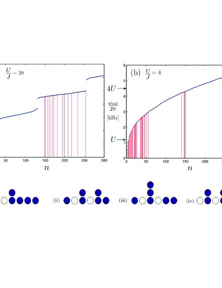
Figure 1: The energy spectra for the first 300 eigenstates $n$ for (a) $U/J=20$ MI regime, and (b) $U/J=4$ SF regime. In both cases the vertical (red) lines denote the presence of a matrix element $|\left\langle n\left|H_{J}\right|0\right\rangle|$ connecting an excited state to the groundstate which is of order $\mathcal{O}(J/U)$ or above. In (c) a schematic depiction of the excitations which exist in the (i) $U$-, (ii) $2U$- and (iii-iv) $3U$-Hubbard bands of the MI regime in (a) is given.

We first consider the modulation scheme with a weak amplitude $A=0.01$ where linear-response is applicable. In figure 2 (a) the total energy of the system $\epsilon$ is shown after the modulation as a function of $\Omega$ for the MI regime with $U/J=20$. As expected from the matrix elements $\left\langle n\left|H_{J}\right|0\right\rangle$ in figure 1(a) there is strong response centred around $U$ spread by the width of the $U$-Hubbard band which is approximately $10J\sim 0.8$ [kHz], and a smaller (barely visible) response at $3U$. The linear response predictions based on equation (5) are shown also and agree well. For the largest peak the growth of energy over the modulation time is shown in figure 2(b) and the slight overestimation of the energy by linear-response is evident at later times. The same calculation for the SF regime with $U/J=4$ is shown in figure 2(b). Again the results of linear-response agree well and the structure follows that of perturbation matrix elements with a broader response between $U$ and $3U$ and an equivalent strength resonance at $4U$.

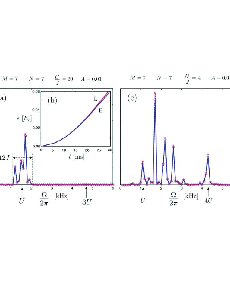
Figure 2: For a weak modulation of the small system we have (a) the total energy $\epsilon$ absorbed in the MI regime with $U/J=20$ as a function of $\Omega$, (b) $\epsilon$ over time for the largest MI peak at $\Omega/2\pi\sim 1.7$ [kHz] for the exact (E) and linear-response (L) calculations, and (c) $\epsilon$ against $\Omega$ for the SF regime with $U/J=4$. In (a) and (c) the markers (o) and (*) denote the exact and linear response results respectively, while the lines are drawn to guide the eye.

In line with the experiment [6] from this point on we consider much stronger modulations with $A=0.2$. The result of these for the MI and SF regimes is given in figure 3. For the MI in figure 3(a) we see that the discrete resonances around $U$ have now filled out into a single peak centred on $U$ that is about 25% wider than the $U$-Hubbard band at $\sim 1$ [kHz], and that the stronger modulation has now increased height of the $3U$ peak relative to the $U$ peak. In figure 3(a) we have also included both first- and second-order perturbation theory results. For such strong modulations the applicability of perturbation theory is highly questionable, especially for the long times considered here. This is exemplified by the gross overestimation of the central peak at $U$ by both linear- and quadratic-response. In figure 3(b) curve (i) shows the saturation of energy absorption for the central peak at $U$ and departure from linear response after a short time. In contrast for the peak at $3U$ figure 3(b) curve (ii) shows that linear-response underestimates the energy absorbed due to its neglect of the role these eigenstates play in the indirect processes to higher energies. However, the use of quadratic-response given by equation (6) provides some useful insight into the additional structure seen for the strong modulation which do not appear for weak modulations and is not predicted by linear-response. Specifically, the small satellite peaks either side of the dominant peak at $U$, which are located at $U/2$ and $3U/2$ respectively, only appear at second and higher order leading to their natural identification as the absorption of two quanta of energy $\Omega$ from the perturbation to reach to $U$- and $3U$-Hubbard bands. We note also that even under strong modulations no resonance at $2U$ is seen in agreement with recent findings [28] for commensurate systems. For the SF regime in figure 3(c) a broad response is seen spanning the region between $U$ and $3U$ consistent with linear response, but higher-order effects have resulted in saturation and merging of linear response peaks. As with weaker modulations there is a separate resonance centred at $4U$ which is now as equivalent in strength and broader.

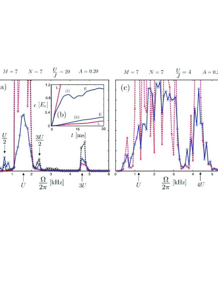
Figure 3: For a strong modulation of the small system we have (a) the total energy $\epsilon$ absorbed in the MI regime with $U/J=20$ as a function of $\Omega$, (b) $\epsilon$ over the time at the MI peaks (i) $U$ and (ii) $3U$ for the exact (E) and linear-response (L) calculations, and (c) $\epsilon$ against $\Omega$ in the SF regime with $U/J=4$. For (a) and (c) the markers (o), (*) denote the exact and linear-response results respectively, while in (a) ($\Diamond$) denotes the quadratic-response. The lines are drawn to guide the eye.

With the full exact calculation we have computed the response of the system for a sequence of depths $U/J=2,3,\dots,20$ which are displayed in figure 4 (a) demonstrating the evolution of the MI spectrum in figure 3 (a) into SF spectrum in figure 3 (c) with decreasing lattice depth. By examining the accompanying colour-map in figure 4 (b) we can make a number of initial observations regarding the changing characteristics of the spectrum over the SF-MI transition. Firstly, as with the weak modulations, the MI peak at $U$ is seen to broaden and shift upwards in energy into the SF response, and this change is most prominent after the depth is lower than $U/J\sim 12$. Secondly, it is now clear that the resonance at $3U$ for deep in the MI regime reduces only slightly in energy and ends up as the $4U$ resonance in the SF regime. Additionally, in line with weaker modulations in figure 2, the $4U$ peak is stronger than the $3U$ peak it evolves from, and signatures of this change are already visible in figure 4 (a). Finally, by progressing to slightly shallower depths ($U/J=2,3$) in figure 4 we see the broadening of the SF spectrum over the entire frequency range considered caused by the eventual merging of the $U$ to $3U$ response with the $4U$ peak.

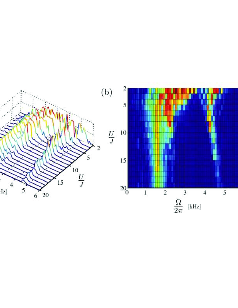
Figure 4: (a) The total energy $\epsilon$ absorbed by a small box system over a sequence of depths, ranging from the MI to SF regimes, as a function of $\Omega$ for strong modulations. (b) A colour-map of plot (a).

4.2 Large system in a box

To put some of the observations made in the previous section on a firmer footing we now examine a larger system with $M=41$ and $N=41$, again with box boundaries, under the same modulation scheme with $A=0.2$. To compute the dynamical evolution for this system we resort to the TEBD algorithm using a lattice site dimension $d_{s}=5$. In figure 5 the one-particle density matrix $\rho_{jk}=\langle b^{\dagger}_{j}b_{k}\rangle$ for the groundstate of (a) the MI with $U/J=20$ and (b) the SF with $U/J=5$ is plotted, along with the corresponding spectra obtained from these groundstates in (c) and (d) respectively. As might be expected the increase in the size of the system reduces finite size effects resulting in much smoother excitation profiles. However, the essential features of these plots still follow directly from our analysis of a small system in terms of both the position and width of the resonances. Specifically, the width of the $U$ peak in figure 5(c) is again slightly larger than the width of the $U$-Hubbard band for this system given approximately by first order perturbation theory as $12J\sim 1$ [kHz]. The effects of saturation also appear to follow similarly with the maximum energy absorbed per particle being nearly identical for the two system sizes.

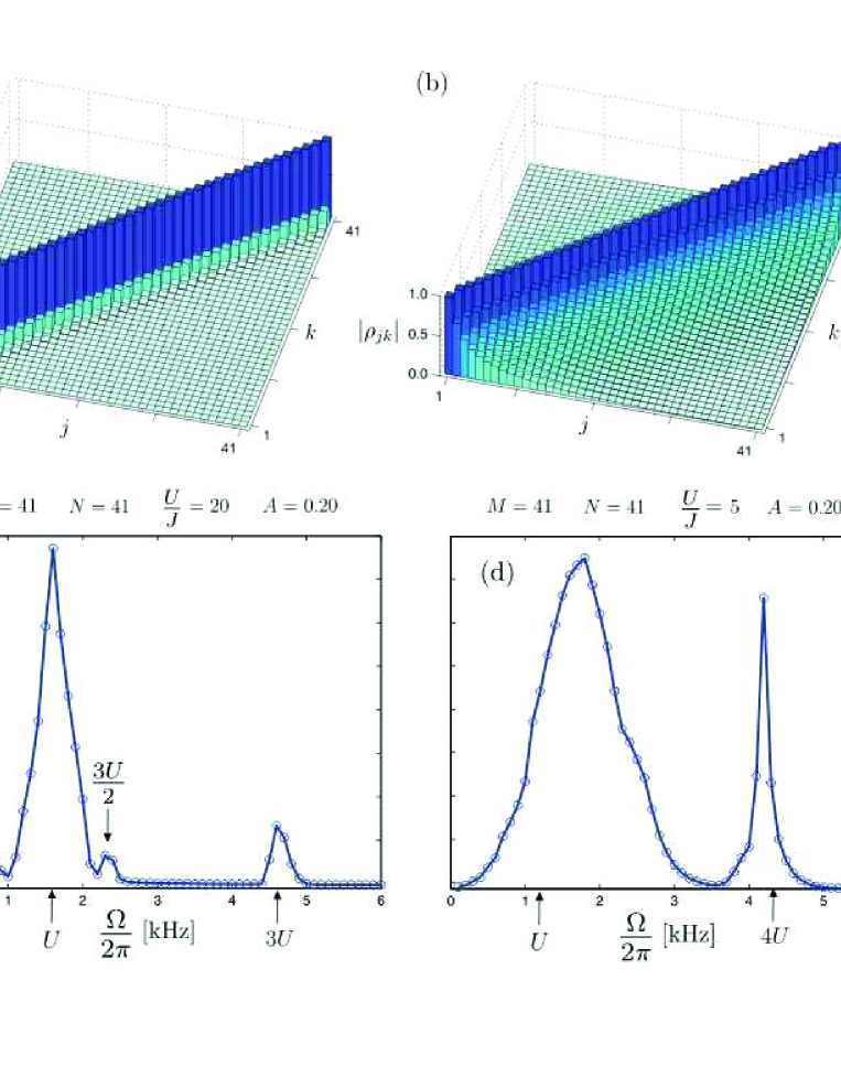
Figure 5: The one-particle density matrix $\rho_{jk}$ of the groundstate for (a) the MI regime with $U/J=20$ and (b) the SF regime with $U/J=5$. The corresponding excitation spectra of the total energy $\epsilon$ against $\Omega$ for these groundstate is shown in (c) and (d) respectively.

The absorption spectrum over a sequence of depths $U/J=5,6,\dots,20$ ranging from the SF to MI regime are shown in figure 6. The increased size of the system permits us to investigate more conclusively some of the observations made earlier regarding the evolution of the absorption spectra with decreasing depth. Firstly, we focus on the maximum strength of the $3U\rightarrow 4U$ peak with $U/J$ which is shown in figure 7 (a). The plot shows that the strength of this peak displays a distinct alteration in its behavior close to $U/J\sim 10$ where it jumps from an increasing to a decreasing curve. This behaviour is consistent with what was seen earlier for the small system and can be attributed to the increasing SF character with a strong $4U$ peak becoming dominant over the weaker $3U$ MI peak.

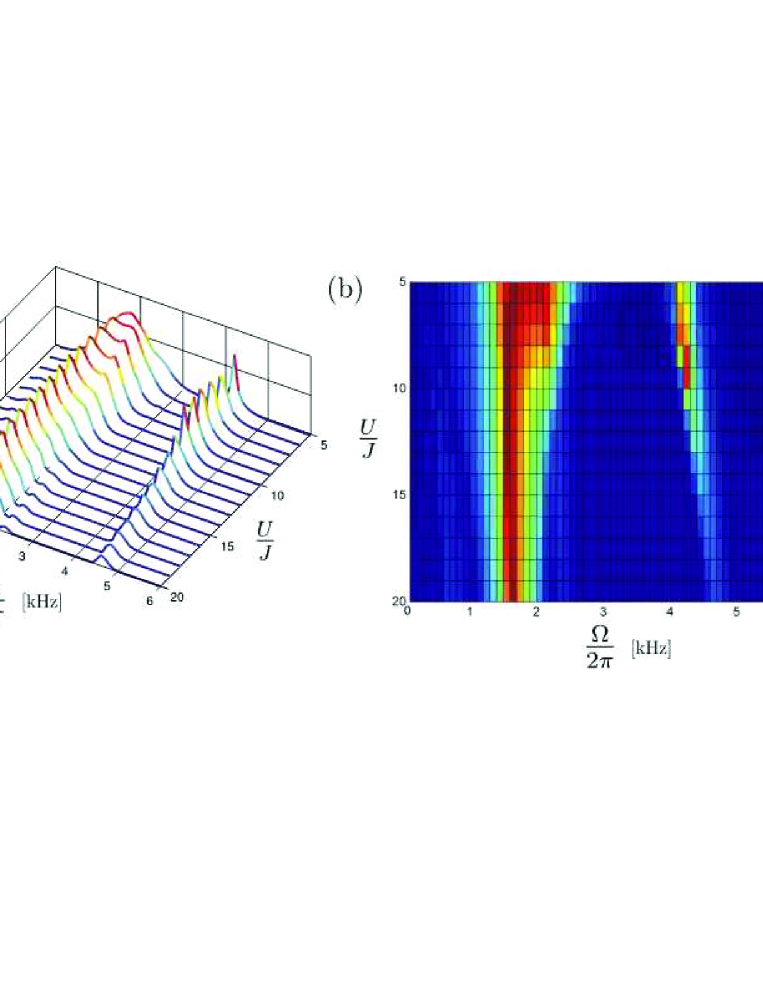
Figure 6: (a) The total energy $\epsilon$ absorbed by a large box system over a sequence of depths, ranging from the MI to SF regimes, as a function of $\Omega$ for strong modulations. (b) A colour-map of plot (a).

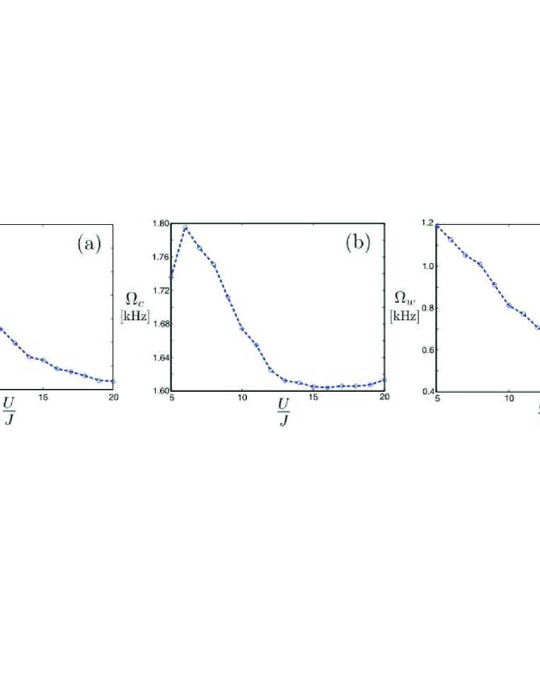
Figure 7: (a) The maximum energy $\epsilon$ absorbed for the $3U\rightarrow 4U$ peak with the lattice depth $U/J$. (b) The centre position $\Omega_{c}$, and (c) width $\Omega_{w}$ of the $U$ resonance with the lattice depth $U/J$. The dotted lines in all cases is drawn to guide the eye.

To understand the changes exhibited by the resonance around $U$ we fit this peak with a smoothed-box function of the form

$$\epsilon(\Omega)=\epsilon_{\textrm{min}}+\mathcal{N}\frac{\epsilon_{\textrm{max}}-\epsilon_{\textrm{min}}}{1+e^{[(\Omega-\Omega_{c})^{2}-w^{2}]/s^{2}}},$$ (7)

where $\Omega_{c}$, $w$ and $s$ are parameters specifying the center, top width and step size of the profile respectively, whilst $\mathcal{N}=1+e^{-w^{2}/s^{2}}$ is the scaling factor. The advantages of this function (which are even more apparent in the next section) is that it faithfully describes both the width and centre location of broad topped resonances. The centre $\Omega_{c}$ and the full-width-half-maximum $\Omega_{w}$ extracted from this fitting then characterizes quantitatively the behaviour which is evident in figure 6 (b).

In figure 7 (b) we see that the centre $\Omega_{c}$ of the $U$ peak remains relatively stationary until $U/J\sim 12$ where it then shifts more dramatically to higher energies. This is again a signature of increasing SF character consistent with the disappearance of the gap between the $U$- and $2U$-Hubbard bands and the shifting of the strongest contributions to $\left\langle n\left|H_{J}\right|0\right\rangle$ to higher frequency seen for the small system. The width $\Omega_{w}$ in figure 7 (c) instead displays a gradual increase without any pronounced changes.

It is clear from the structure of both the MI and SF spectra shown in figure 5(c) and (d) that the box system has some differences compared to the 1D spectra obtained in the experiment. These differences are not surprising given that the SF state of the box system at $U/J=5$ exhibits significant quantum depletion of $75\%$, which is much larger than that in the experiment. Also, at all depths considered here the groundstate of the box has a near homogeneous density of 1 atom per site, as can be seen in figure 5(a) and (b), which is different from the harmonically trapped system in the experiment.

4.3 Large harmonically trapped system

To approach a setup closer to that of the experiment we now consider a system with $M=25$ and $N=15$ superimposed with harmonic trapping using $\omega_{T}/2\pi=70$ Hz. A significant difference is that at $U/J=5$ the depletion of the SF state is reduced to $50\%$ in line with the experiment for this setup. The one-particle density matrices for the MI and SF groundstates in this case are shown in figure 8(a) and (b) respectively. We now see that the MI state is composed of a central core with unit filling along with small SF lobes at the edges. This change in structure compared to figure 5(a) introduces additional types of excitations such as those caused by particles hopping into the vacuum surrounding the MI core. For the SF state there are now significantly greater off-diagonal correlations in $\rho_{jk}$ compared to the box system. Despite these differences, however, the form of the spectrum shown in figure 8(c) and (d) remains very close to the box system displaying the same characteristic peaks as before. The effects of trapping manifest themselves in this case by flattening of the $U$ peak, along with the broadening and shifting of the $4U$ peak. The maximum energy per particle again remains approximately equal to the previous cases considered, showing that the saturation effects are not significantly altered by the trapping.

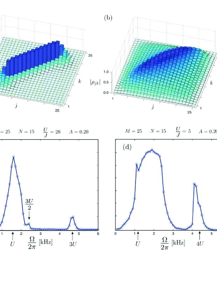
Figure 8: The one-particle density matrix $\rho_{jk}$ of the groundstate for a trapped system with $\omega_{T}/2\pi=70$ Hz for (a) the MI regime with $U/J=20$ and (b) the SF regime with $U/J=5$. The corresponding excitation spectra of the total energy $\epsilon$ against the modulation frequency $\Omega$ for these groundstate are shown in (c) and (d) respectively.

In figure 9 we report the spectra for the system ranging over SF to MI regimes as before. Again, the essential features of this plot follow from our earlier discussion. Performing the same analysis on the evolution of the spectrum demonstrates that maximum strength of the $3U\rightarrow 4U$ peak has a maximum at $U/J\sim 8$ as shown in figure 10(a). The trapping is also seen to introduce peaks and troughs to this curve compared to the smooth behaviour of the box system. Also, in contrast to the box both the centre $\Omega_{c}$ and width $\Omega_{w}$ of the $U$ resonance show a gradual change from the MI to SF character in figure 10(b) and (c). This reflects a difference in the evolution of $U$ resonance, which for the box develops a visible two-peaked structure in figure 6(a), whereas in the harmonic trap this is washed out into a broader and flatter response in figure 9(a).

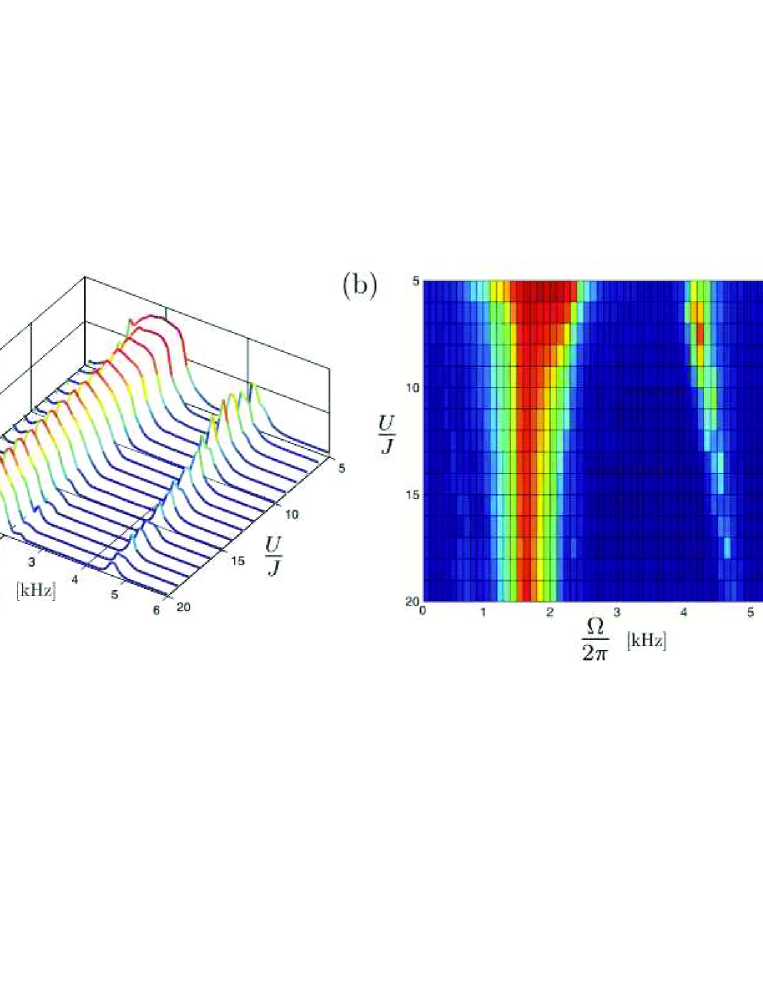
Figure 9: (a) The total energy $\epsilon$ absorbed by a $M=25$ and $N=15$ harmonically trapped system over a sequence of depths, ranging from the MI to SF regimes, as a function of $\Omega$ for strong modulations. (b) A colour-map of plot (a).

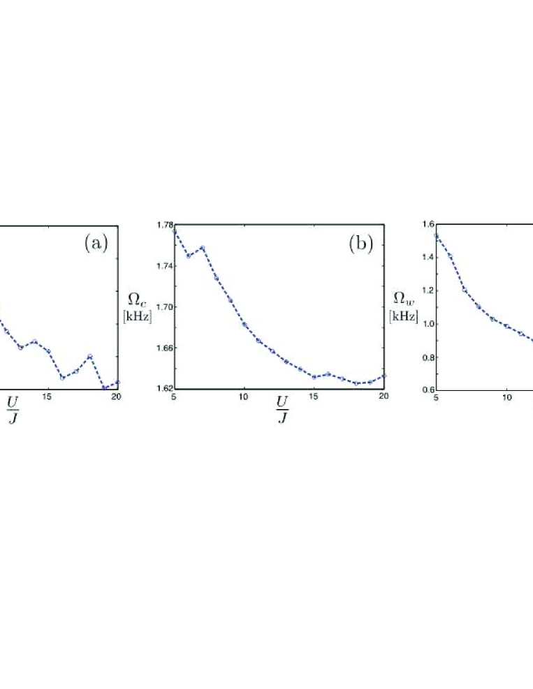
Figure 10: (a) The maximum energy $\epsilon$ absorbed for the $3U\rightarrow 4U$ peak with the lattice depth $U/J$. (b) The centre position $\Omega_{c}$, and (c) width $\Omega_{w}$ of the $U$ resonance with the lattice depth $U/J$. The dotted lines in all cases is drawn to guide the eye.

We have seen that the introduction of harmonic trapping for the case considered above has not lead to any new features in the spectrum beyond a small amount of shifting and broadening. One such feature which might be expected is the emergence of a resonance at $2U$. However, it is known that the relevant excitation processes for a $2U$ resonance require either excitations to already be present in the system due to finite temperature [13], or significant inhomogeneity in the density caused by a trap [28]. Since the system above is at $T=0$ and has virtually no incommensurability in the MI, beyond the small SF lobes at the edges, the lack of a $2U$ resonance is consistent. In the experiment both finite-temperature and inhomogeneity are expected to make important contributions to the spectrum. Presently there are still open questions as to which is the most dominant and what interplay there might be between these effects. Future studies with the TEBD algorithm, exploiting recent developments which permit the simulation of master equation evolution of 1D finite-temperature and dissipative systems [49], could allow both these effects to be treated on an equal footing.

To demonstrate the contribution of inhomogeneity we have performed additional calculations again using $M=25$ but with a larger occupancy of $N=30$ and larger trapping frequency $\omega_{T}/2\pi=100$ Hz. In figure 11(a) the one-particle density matrix of the MI groundstate at $U/J=20$ is shown and displays the coexistence of significant MI and SF regions characteristic of trapped systems. Despite using a larger lattice site dimension $d_{s}=6$ for this setup we found that truncation in on-site occupancy limited the smallest $U/J$ from which we could reliably compute the spectrum to $U/J=9$. The one-particle density matrix for the $U/J=9$ groundstate is shown in figure 11(b) and appears to be dominated by a central SF region. The excitation spectra for these two groundstates are shown in figure 11(c) and (d) respectively. For the MI in figure 11(c) a pronounced $2U$ resonance is seen in addition to the peaks seen in previous MI spectra. The appearance of a $2U$ peak in the $T=0$ case examined here arises predominantly from particles in the unit filled MI shell hopping into the doubly occupied region at the centre [28, 6] which is evident in the one-particle density matrix shown in figure 11(a). For the shallower depth $U/J=9$ the spectrum in figure 11(d) exhibits the initial merging of the $U$ and $4U$ peaks with this $2U$ peak. In figure 12 the evolution of the spectrum between these limits is shown. The form of these spectra is very reminiscent of that shown in the experiment [6] and it is likely that a more detailed analysis of this setup to shallower lattice depths would reveal the broad SF resonance seen experimentally.

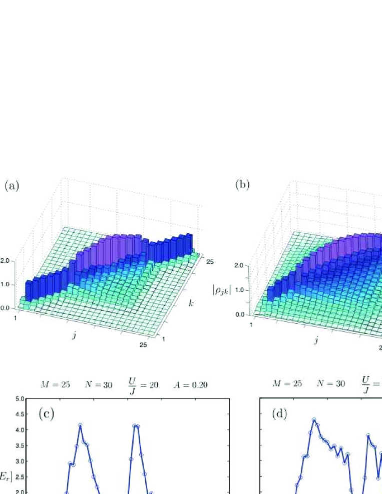
Figure 11: The one-particle density matrix $\rho_{jk}$ of the groundstate for a trapped system with $\omega_{T}/2\pi=100$ Hz for (a) the MI regime with $U/J=20$ and (b) an intermediate regime with $U/J=9$. The corresponding excitation spectra of the total energy $\epsilon$ against the modulation frequency $\Omega$ for these groundstate are shown in (c) and (d) respectively.

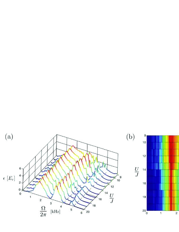
Figure 12: (a) The total energy $\epsilon$ absorbed by a $M=25$, $N=30$ harmonically trapped system over a sequence of depths, ranging from the MI to SF regimes, as a function of $\Omega$ for strong modulations. (b) A colour-map of plot (a).

5 Conclusions

We have examined in detail the dynamical response at $T=0$ of the ultracold atoms in an optical lattice subjected to lattice modulations. We have reported the evolution of the excitation spectrum with the lattice depth from the SF to MI regime for small and large box systems, and for large harmonically trapped systems. For the box system we identified two pronounced signatures of the transition from the MI to SF regime, specifically the strength of the $3U\rightarrow 4U$ peak and the centre of the $U$ resonance. The introduction of trapping for the case considered here, where the occupancy remains less than or equal to unity, does not significantly alter the evolution of the spectrum compared to a box system. While we find that it does wash out any pronounced changes in the structure of the $U$ resonance with depth, the strength of the $3U\rightarrow 4U$ peak still exhibits a signature of increasing SF character.

We also presented calculations showing spectra progressing from the MI regime for a harmonically trapped system which has a central region with greater than unit filling. We found that this changes the structure of the spectrum by introducing a $2U$ resonance and brings our results closer with the experiment. Direct comparison to the experiment [6], however, is difficult due to the 3D rethermalization performed prior to measurement, which cannot be simulated with TEBD, and the fact that the measurement itself was an averaged result over many 1D systems in parallel with differing total particle number. Despite this our results point to that fact that the BHM is sufficient to explain all the features discovered in the experiment and that the experiment was a clean realization of this model as expected.

References

References

- [1] Greiner M, Mandel O, Esslinger T, Hänsch T W and Bloch I 2002 Nature 415 39
- [2] Fisher M P A, Weichman P B, Grinstein G and Fisher D S 1989 Phys. Rev. B 40 546
- [3] Jaksch D, Bruder C, Cirac J I, Gardiner C W and Zoller P 1998 Phys. Rev. Lett.81 3108
- [4] Paredes B, Widera A, Murg V, Mandel O, Fölling S, Cirac J I, Shlyapnikov G V, Hänsch T W and Bloch I 2004 Nature 429 277
- [5] Kinoshita T, Wenger T and Weiss D S, 2004 Science 305 1125
- [6] Stöferle T, Moritz H, Schori C, Köhl M and Esslinger T 2004 Phys. Rev. Lett.92 130403
- [7] Köhl M, Moritz H, Stöferle T, Schori C and Esslinger T 2005 J. Low Temp. Phys. 138 635
- [8] Günter K, Stöferle T, Moritz H, Köhl M and Esslinger T Preprint Phys. Rev. Lett.96 180402
- [9] Ospelkaus S, Ospelkaus C, Wille O, Succo M, Ernst P, Sengstock K and Bongs K 2006 Phys. Rev. Lett.96 180403
- [10] Roth R and Burnett K 2004 J. Phys. B 37 3893
- [11] Batrouni G G, Assaad F F, Scalettar R T, and Denteneer P J H 2005 Phys. Rev. A 72 031601(R)
- [12] Rey A M, Blakie Blair P, Pupillo G, Williams C J and Clark C W 2005 Phys. Rev. A 72 023407
- [13] Reischl A, Schmidt K P and Uhrig G S 2005 Phys. Rev. A 72 063609
- [14] Giamarchi T 2004 Quantum Physics in One Dimension (Oxford University Press, Oxford)
- [15] Menotti C, Krämer M, Pitaevskii L and Stringari S 2003 Phys. Rev. A 67 053609
- [16] Büchler H P and Blatter G 2003 Preprint cond-mat/0312526
- [17] Krämer M, Tozzo C and Dalfovo F 2004 Phys. Rev. A 71 061602(R)
- [18] Tozzo C, Krämer M and Dalfovo F 2005 Phys. Rev. A 72 023613
- [19] Iucci A, Cazilla M A, Ho A F and Giamarchi T 2006 Phys. Rev. A 73 041608
- [20] Mandel O, Greiner M, Widera A, Rom T, Hänsch T W and Bloch I 2003 Nature 425 937
- [21] Jaksch D, Briegel H-J, Cirac J I, Gardiner C W and Zoller P 1999 Phys. Rev. Lett.82 1975
- [22] Dorner U, Fedichev P, Jaksch D, Lewenstein M and Zoller P 2003 Phys. Rev. Lett.91 073601
- [23] Pachos J K and Knight P L 2003 Phys. Rev. Lett.91 107902
- [24] Brennen G K, Caves C M, Jessen P S and Deutsch I H 1999 Phys. Rev. Lett.82 1060
- [25] Clark S R, Moura-Alves C and Jaksch D 2005 New J. Phys.7 124
- [26] Jane E, Vidal G, Dür W, Zoller P and Cirac J I 2003 Quantum Info. and Comp. 3 15
- [27] Sörensen A and Mölmer K 1999 Phys. Rev. Lett.83 2274
- [28] Kollath C, Iucci A, Giamarchi T, Hofstetter W and Schollwöck U Preprint cond-mat/0603721
- [29] Jaksch D and Zoller P 2004 Ann. Phys. 315 52
- [30] Moritz H, Stöferle T, Köhl M and Esslinger T 2003 Phys. Rev. Lett.91 250402
- [31] Zwerger W 2003 J. Opt. B; Quantum Semiclassical Opt. 5 9
- [32] Sachdev S 2001 Quantum Phase Transitions (Cambridge University Press, Cambridge).
- [33] Kühner T and Monien H 1998 Phys. Rev. B 58 R14741
- [34] Batrouni G G, Rousseau V, Scalettar R T, Rigol M, Muramatsu A, Denteneer P J H and Troyer M 2002 Phys. Rev. Lett.89 117203
- [35] For the exact system we consider shallow depths which are strictly beyond the validity of the tight-binding lowest-band BHM. However, these still provide important information regarding the evolution of the excitation spectrum at shallow depths.
- [36] Vidal G 2003 Phys. Rev. Lett.91 147902
- [37] Vidal G 2004 Phys. Rev. Lett.93 040502
- [38] Clark S R and Jaksch D 2004 Phys. Rev. A 70 043612
- [39] Daley A J, Kollath C, Schollwöck U and Vidal G 2004 J. Stat. Mech.: Theor. Exp. P04005
- [40] Daley A J, Clark S R, Jaksch D and Zoller P 2005 Phys. Rev. A 72 043618
- [41] Gobert D, Kollath C, Schollwöck U and Schütz G 2005 Phys. Rev. E 71 036102
- [42] Kollath C, Schollwöck U, von Delft J and Zwerger W 2005 Phys. Rev. A 71 053606
- [43] White S R and Feiguin A E 2004 Phys. Rev. Lett.93 076401
- [44] White S R 1992 Phys. Rev. Lett.69 2863; 1993 Phys. Rev. B 48 10345
- [45] Schollwöck U 2005 Rev. Mod. Phys. 77 259
- [46] Krauth W, Caffarel M and Bouchaud J P 1992 Phys. Rev. B 45 3137
- [47] Bañuls M C, Orús R, Latorre J I, Pérez A and Ruiz-Femenía P 2006 Phys. Rev. A 73 022344
- [48] Braun-Munzinger K, Dunningham J A and Burnett K 2004 Phys. Rev. A 69 053613
- [49] Zwolak M and Vidal G 2004 Phys. Rev. Lett.93 207205