Optically controlled spin-glasses in multi-qubit cavity systems

Abstract

Recent advances in nanostructure fabrication and optical control, suggest that it will soon be possible to prepare collections of interacting two-level systems (i.e. qubits) within an optical cavity. Here we show theoretically that such systems could exhibit novel phase transition phenomena involving spin-glass phases. By contrast with traditional realizations using magnetic solids, these phase transition phenomena are associated with both matter and radiation subsystems. Moreover the various phase transitions should be tunable simply by varying the matter-radiation coupling strength.

PACS numbers: 42.50.Fx, 75.10.Nr, 32.80.-t

Condensed matter physicists are keen to identify experimental realizations of Ising-like Hamiltonians involving populations of interacting two-level objects (i.e. spins) Kad . Exotic phases such as a spin-glass are of particular interest Sherr . Experimental studies of spin-glasses have focused on solids containing arrays of magnetic ions Kad . However the laws of Nature limit the range of exotic behaviors that such solids can exhibit, since it is very hard to engineer the magnitude, anisotropy, range and/or disorder of the spin-spin interaction in such systems. In the seemingly unrelated fields of atomic, nanostructure and optical physics, there have been rapid advances in the fabrication and manipulation of effective two-level systems (more commonly referred to as qubits) using atoms, semiconductor quantum dots, and superconducting nanostructures NatQED ; review ; QDcavity ; ima ; books ; QD . In particular, controlled qubit-cavity coupling has been demonstrated experimentally between such systems and a surrounding optical cavity NatQED ; review ; QDcavity ; ima ; books ; QD ; PBG . In quantum dots systems, in particular, the effective spin-spin (i.e. qubit-qubit) interaction can in principle be tailored by adjusting the quantum dots’ size, shape, separation, orientation and the background electrostatic screening. Furthermore, the interaction’s anisotropy can be engineered by choosing asymmetric dot shapes. Disorder in the qubit-qubit interactions will arise naturally for self-assembled dots, or can be introduced artificially by varying the individual dot positions during fabrication QD ; jopa .

Motivated by these recent experimental advances, we study the phase transitions which could arise in such multi-qubit-cavity systems. We uncover novel realizations of spin-glasses Sherr in which the phase transition phenomena are associated with the spin (i.e. matter) and boson (i.e. photon) subsystems. The resulting phase diagrams can be explored experimentally by varying the qubit-cavity coupling strength $\lambda$, e.g. by re-positioning the center of the cavity around the nanostructure array, changing its orientation, or tuning the cavity Q-factor NatQED . In addition to opening up the study of these important condensed matter systems to the nano-optical community, our results help strengthen the theoretical connection which seems to be emerging between multi-qubit-cavity systems and spin-spin systems CMP ; CFL .

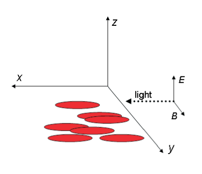
Figure 1: (color online) Schematic diagram showing a possible optical realization of a spin-glass system within a multi-qubit-cavity system comprising elongated quantum dots. The quantum dots are orientated along the $x$-axis and have non-uniform spacings, giving rise to disorder in the qubit-qubit interaction $\{J_{ij}\}$.

Given the above experimental considerations, we will introduce a generalization of the well-known Dicke model CMP ; CFL ; Dic54 ; WH73 in order to describe $N$ interacting two-level systems in a cavity field:

$$H = a^{\dagger}a+H_{I}+\frac{\epsilon}{2}\sum_{i=1}^{N}\sigma_{i}^{z}+\frac{\lambda}{2\sqrt{N}}\sum_{i=1}^{N}(\sigma_{i}^{+}+\sigma_{i}^{-})(a+a^{\dagger}),$$

where the operators $a,a^{\dagger}$ and $\sigma^{\pm}_{j},\sigma^{Z}_{j}$ correspond to the photon field and quantum dot $j$ respectively. The interaction term $H_{I}=\sum_{i<j}J_{ij}\sigma_{i}^{z}\sigma_{j}^{z}$ or $H_{I}=\sum_{i<j}J_{ij}\sigma_{i}^{x}\sigma_{j}^{x}$ (or equivalently $\sum_{i<j}J_{ij}\sigma_{i}^{y}\sigma_{j}^{y}$). An interaction in the $z$-direction is present naturally review . In the case of the $x$-directed interaction, each quantum dot can be engineered to have an elongated form along the $x$-direction, by biasing the growth process along this direction. Applying an electric field along $x$, will then create large dipole moments in that direction. One can use undoped dots, in which case the dipole results from the exciton, or doped dots, in which case the dipole originates from the conduction-subband electron biased along $x$. A schematic plot of a possible realization is depicted in Fig. 1. Kiraz et al. QDcavity , for example, have already built physical realizations of such multi-qubit-cavity nanostructure systems. In particular, Ref. QDcavity shows a scanning electron micrograph of the GaAs microdisk nanostructure system comprising a disordered array of quantum dots embedded within an optical cavity. The cavity has a diameter of $4.5\mu m$ and produced Q-factor values exceeding 1800 QDcavity . The cavity was built with a collection of InAs quantum dots at irregular locations fixed during the growth, and hence necessarily features disordered dot-dot couplings $\{J_{ij}\}$. Another suitable experimental set-up has been provided by Imamoglu et al. ima in which a quantized cavity mode and applied laser fields are used to mediate the interaction between spins of distant, doped quantum dots. This leads to cavity-assisted spin-flip Raman transitions and hence pairs of quantum dots can be coupled via virtual photons in the common vacuum cavity mode ima ; review .

The dot-dot coupling terms $\{J_{ij}\}$ will have an inherent disorder in self-assembled dots – alternatively, such disorder can be built in during growth by varying the dot-dot separations. We make the reasonable assumption Sherr that the disorder will be Gaussian:

$$P(J_{ij})=\left(\frac{N}{2\pi J^{2}}\right)^{\frac{1}{2}}{\rm exp}\left(-\frac{J_{ij}^{2}N}{2J^{2}}\right)\ \ .$$

First we consider $H_{I}=\sum_{i<j}J_{ij}\sigma_{i}^{z}\sigma_{j}^{z}$, noting that the same method can then be used to solve for spin–spin interactions in the other directions. To obtain the thermodynamical properties of the system, we introduce the Glauber coherent states $|\alpha\rangle$ of the field Glauber where $a|\alpha\rangle=\alpha|\alpha\rangle$, $\langle\alpha|a^{\dagger}=\langle\alpha|\alpha^{*}$. The coherent states are complete, $\int\frac{d^{2}\alpha}{\pi}|\alpha\rangle\langle\alpha|=1$. In this basis, we may write the canonical partition function as:

$$Z(N,T)=\sum_{\bf s}\int\frac{d^{2}\alpha}{\pi}\langle{\bf s}|\langle\alpha|e^{-\beta H}|\alpha\rangle|{\bf s}\rangle.$$

As in Ref. WH73 , we adopt the following assumptions:

1. $a/\sqrt{N}$ and $a^{\dagger}/\sqrt{N}$ exist as $N\rightarrow\infty$;

2. $\lim_{N\rightarrow\infty}\lim_{R\rightarrow\infty}\sum_{r=0}^{R}\frac{(-\beta H_{N})^{r}}{r!}$ can be interchanged.

We then obtain:

$$Z = {\rm Tr\ }e^{-\beta H}$$

$$= \int\frac{d^{2}\alpha}{\pi}{\rm Tr\exp}\bigg{\{}-\beta\Big{(}{\rm Re}(\alpha)^{2}+{\rm Im}(\alpha)^{2}$$

$$+\sum_{i<j}J_{ij}\sigma_{i}^{z}\sigma_{j}^{z}+\frac{\epsilon}{2}\sum_{i=1}^{N}\sigma_{i}^{z}+\frac{2\lambda}{\sqrt{N}}{\rm Re}(\alpha)\sum_{i=1}^{N}\sigma_{i}^{x}\Big{)}\bigg{\}}.$$

Performing the Gaussian integration of ${\rm Im}(\alpha)$ and setting $w={\rm Re}(\alpha)$ yields the partition function:

$$Z = {\rm Tr\exp}\bigg{\{}-\beta\Big{(}w^{2}+\sum_{i<j}J_{ij}\sigma_{i}^{z}\sigma_{j}^{z}+\frac{\epsilon}{2}\sum_{i=1}^{N}\sigma_{i}^{z}$$

$$\qquad\qquad\qquad+\frac{2\lambda w}{\sqrt{N}}\sum_{i=1}^{N}\sigma_{i}^{x}\Big{)}\bigg{\}}.$$

We set $J_{ij}\rightarrow-J_{ij}$, $\epsilon=-2\mu$ and $\lambda=-\frac{\Gamma}{2}$ for convenience and rescale the photon field $a^{\dagger}\rightarrow\sqrt{N}b^{\dagger}$ such that $w\rightarrow\sqrt{N}W$. We then use the Trotter-Suzuki method Thirumalai , and obtain the free energy from the replica trick:

$$-\beta F=[\ln(Z)]=\lim_{n\rightarrow 0}\frac{[Z^{n}]-1}{n}$$

where $[Z^{n}]$ is the configurational average of the $n$ replicated partition functions. Rewriting the trace and using the method of steepest descents, we can proceed in the usual manner for spin-glass problems. In the thermodynamic limit $N\to\infty$, with the limit $n\to 0$ with $N$ kept large but finite, we obtain the free energy, $f=\frac{F}{N}$, as:

$$-\beta f = \lim_{\shortstack{{\tiny$n\to 0$} \\ {\tiny$P\to\infty$} \\ {\tiny$N\to\infty$}}}\frac{[Z^{n}]-1}{Nn}$$

$$= \lim_{\shortstack{{\tiny$n\to 0$} \\ {\tiny$P\to\infty$} \\ {\tiny$N\to\infty$}}}\Biggr{\{}-\frac{1}{2nP^{2}}\sum_{\alpha,t,t^{\prime}}(x_{tt^{\prime}}^{\alpha\alpha})^{2}-\frac{1}{2nP^{2}}\sum_{(\alpha,\beta),t,t^{\prime}}(y_{tt^{\prime}}^{\alpha\beta})^{2}$$

$$+\frac{1}{n}\ln\biggl{\{}{\rm Tr\exp}\Bigl{\{}\frac{\beta J}{\sqrt{2}P^{2}}\sum_{t,t^{\prime}}\sum_{(\alpha,\beta)}y_{tt^{\prime}}^{\alpha\beta}\sigma_{t}^{\alpha}\sigma_{t^{\prime}}^{\beta}$$

$$+\frac{\beta J}{\sqrt{2}P^{2}}\sum_{t,t^{\prime}}\sum_{\alpha}x_{tt^{\prime}}^{\alpha\alpha}\sigma_{t}^{\alpha}\sigma_{t^{\prime}}^{\alpha}+\frac{\beta\mu}{P}\sum_{t}\sum_{\alpha}\sigma_{t}^{\alpha}$$

$$-\frac{\beta}{P}\sum_{t}\sum_{\alpha}(W^{\alpha})^{2}$$

$$+\sum_{t}\sum_{\alpha}\omega^{\alpha}\left(C^{\alpha}+\sigma_{t}^{\alpha}\sigma_{t+1}^{\alpha}\right)\Bigr{\}}\biggr{\}}\Biggr{\}},$$

with $\alpha$ being the replica index and $t=1,2,3,\cdots,P$ the label for the Trotter direction. We then substitute for the following stationary values:

$$x_{tt^{\prime}}^{\alpha\alpha} = \frac{1}{\sqrt{2}}\beta J\langle\sigma_{\alpha}^{t}\sigma_{\alpha}^{t^{\prime}}\rangle\equiv\frac{1}{\sqrt{2}}\beta J\chi_{tt^{\prime}}^{\alpha\alpha}$$

$$y_{tt^{\prime}}^{\alpha\beta} = \frac{1}{\sqrt{2}}\beta J\langle\sigma_{\alpha}^{t}\sigma_{\beta}^{t^{\prime}}\rangle\equiv\frac{1}{\sqrt{2}}\beta Jq_{tt^{\prime}}^{\alpha\beta}.$$

The replica symmetric assumption Thirumalai yields $\chi_{tt^{\prime}}^{\alpha\alpha}=\chi_{tt^{\prime}}$, $q_{tt^{\prime}}^{\alpha\beta}=q_{tt^{\prime}}$, $W^{\alpha}=W$, and with the static approximation we then obtain $\chi_{tt^{\prime}}=\chi$ and $q_{tt^{\prime}}=q$. The validity of this approximation has been discussed at length in Ref. Thirumalai . Hence:

$$-\beta f = \lim_{\shortstack{{\tiny$n\to 0$} \\ {\tiny$P\to\infty$} \\ {\tiny$N\to\infty$}}}\Biggl{\{}-\beta W^{2}-\frac{\beta^{2}J^{2}\chi^{2}}{4}-\frac{\beta^{2}J^{2}(n-1)q^{2}}{4}+\frac{1}{n}\ln\left\{\int Dz_{1}\prod_{\alpha}\int Dz_{2_{\alpha}}{\rm e}^{\left(\sum_{t}\omega C\right)}{\rm Tr\ e}^{\left(\sum_{t}\left(h_{\alpha}\sigma_{\alpha}^{t}+\omega\sigma_{\alpha}^{t}\sigma_{\alpha}^{t+1}\right)\right)}\right\}\Biggr{\}}$$

with

$$h_{\alpha}=\frac{\beta J}{P}\left(\sqrt{q}z_{1}+\sqrt{\chi-q}z_{2_{\alpha}}+\frac{\mu}{J}\right),$$

$\int Dz_{1}=\sqrt{\frac{1}{2\pi}}\int\exp\left\{-\frac{z_{1}^{2}}{2}\right\}$ and $\int Dz_{2_{\alpha}}=\sqrt{\frac{1}{2\pi}}\int\exp\left\{-\frac{z_{2_{\alpha}}^{2}}{2}\right\}$. We then calculate the trace and perform power series expansions in the limit $P\to\infty$. Finally, we expand out the last term in the free energy, take the limit $n\to 0$ and replace $\mu$ and $\Gamma$ by their original values $\mu=-\frac{\epsilon}{2}$ and $\Gamma=-2\lambda$ to obtain:

$$-\beta f = -\beta W^{2}-\frac{\beta^{2}J^{2}}{4}\left(\chi^{2}-q^{2}\right)$$

$$+\int Dz_{1}\ln\left(\int Dz_{2}2\cosh\Omega\right)$$

with

$$\Omega = \left(b^{2}+\beta^{2}\lambda^{2}W^{2}\right)^{\frac{1}{2}},$$

$$b = \beta J\left(\sqrt{q}z_{1}+\sqrt{\chi-q}z_{2}-\frac{\epsilon}{J}\right),$$

having absorbed the factors $\frac{1}{2}$ and $4$ into $\epsilon$ and $\lambda$ respectively. The requirement that the free energy is stationary yields the following self-consistent equations:

$$\chi = \int Dz_{1}\left\{\frac{\int Dz_{2}\left\{\left(\frac{b^{2}}{\Omega^{2}}\right)\cosh\Omega+\left(\frac{\beta^{2}\lambda^{2}W^{2}}{\Omega^{3}}\right)\sinh\Omega\right\}}{\int Dz_{2}\cosh\Omega}\right\},$$

$$q = \int Dz_{1}\left(\frac{\int Dz_{2}\left\{\left(\frac{b}{\Omega}\right)\sinh\Omega\right\}}{\int Dz_{2}\cosh\Omega}\right)^{2},$$

$$W = \frac{1}{2}\int Dz_{1}\left\{\frac{\int Dz_{2}\left(\sinh\Omega\left(\frac{\beta\lambda^{2}W}{\Omega}\right)\right)}{\int Dz_{2}\cosh\Omega}\right\}.$$

Adding $\Delta H=h\sigma_{i}^{z}$ to the Hamiltonian such that $\epsilon\to(\epsilon+h)$ and taking the limit $h\to 0$, yields:

$$m=-\frac{1}{\beta}\frac{\partial f}{\partial h}\bigg{|}_{h=0}=-\int Dz_{1}\left\{\frac{\int Dz_{2}\left\{\left(\frac{b}{\Omega}\right)\sinh\Omega\right\}}{\int Dz_{2}\cosh\Omega}\right\}.$$

Figure 2: A plot of the magnitude of the super-radiant order parameter, $W$, against $\lambda$ with $\beta=2$, $\epsilon=1$ and $J=2$, and a spin–spin interaction in the $z$-direction. The gap between the two non-zero $W$ phases disappears as we decrease the temperature, $T$.

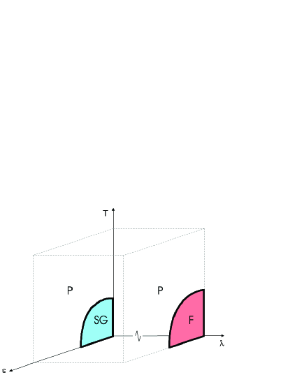
Figure 3: (color online) Schematic plot of the phase diagram of our system when a spin–spin coupling is present in the $x$-direction. As we increase $\lambda$, the phase diagram changes from one which resembles that of an Ising spin-glass model with a transverse field, to one with only ferromagnetic and paramagnetic phases (i.e. the spin-glass phase has disappeared).

An intricate array of phase transitions arises in both the matter and the optical sub-systems. Furthermore, these transitions in the matter and optical sub-systems are inter-dependent. Here we summarize the main results for a general interaction $H_{I}=\sum_{i<j}J_{ij}\sigma_{i}^{z}\sigma_{j}^{z}+\sum_{i<j}J_{ij}\sigma_{i}^{x}\sigma_{j}^{x}$. If the interaction is only in the $z$-direction, a ferromagnetic-paramagnetic phase transition emerges in the matter sub-system – but there is no spin-glass phase anywhere in the phase diagram. This is to be expected, as at any finite value of $\epsilon$ there is a non-zero contribution to the magnetisation as $\epsilon$ acts as a longitudinal term to the Ising interaction Sherr . As such, we would only expect a spin glass phase in the limit of $\epsilon\to 0$. However, novel behavior emerges in the optical sub-system in the form of two sub-superradiant phase transitions, as shown in Fig. 2. This effect disappears as we increase $\beta$. We see that the system goes through a first order and then a second order phase transition as we increase $\lambda$ CFL . In particular, the sharp nature of both transitions and the narrowing of the gap between them as $\beta$ increases, suggests that an accurate low-temperature thermometer could be constructed based on this effect.

The addition of the $x$-directional interaction to the original Dicke Hamiltonian yields a number of interesting results. In particular, the condition for the system to exhibit a sub-superradiant phase transition is drastically changed from the case without interactions. If $J$ is large, the matter sub-system swamps the optical sub-system and the system is unable to reach superradiance. Consequently the magnetization is always zero. However, lowering $J$ yields a superradiant phase – and by varying $\epsilon$ we uncover a spin-glass phase that moves into a paramagnetic phase at higher $\epsilon$. Most remarkably, there are two different phase diagrams for the system depending on the value of the qubit-cavity coupling $\lambda$ at a given $J$. The corresponding phase boundaries are indicated in Fig. 3. The complex behavior in the region between these two limits will be discussed in depth elsewhere.

To summarize, our work shows that novel phase transition phenomena will arise in suitable optical realizations of generalized spin-spin Hamiltonians. In addition to their intrinsic theoretical interest, we hope that our findings might motivate experimental efforts toward exploring these predicted phases.

References

- (1) L.P. Kadanoff, Statistical Physics (World Scientific, Singapore, 2000).
- (2) D. Sherrington and S. Kirkpatrick, Phys. Rev. Lett. 35, 1792 (1975); S. Kirkpatrick and D. Sherrington, Phys. Rev. B, 17, 4384 (1978); M. Mezard, G. Parisi and M.A. Virasoro, Spin Glass Theory and Beyond (World Scientific, Singapore, 1987); H. Nishimori, Statistical Physics of Spin Glasses and Information Processing (Oxford University Press, Oxford, 2001).
- (3) T. Yoshie, A. Scherer, J. Hendrickson, G. Khitrova, H.M. Gibbs, G. Rupper, C. Ell, O.B. Shchekin and D.G. Deppe, Nature 432, 200 (2004); A. Wallraff, D.I. Schuster, A. Blais, L. Frunzio, R.- S. Huang, J. Majer, S. Kumar, S. M. Girvin, R.J. Schoelkopf, Nature 431, 162 (2004); G.R. Guth hrlein, M. Keller, K. Hayasaka, W. Lange, H. Walther, Nature 414, 49 (2001).
- (4) A. Olaya-Castro, N.F. Johnson, quant-ph/0406133, to appear in Handbook of Theoretical and Computational Nanotechnology edited by W. Schommers (2005).
- (5) A. Kiraz, C. Reese, B. Gayral, L.Zhang, W. V. Schoenfeld, B. D. Gerardot, P. M. Petroff, E. L. Hu and A. Imamoglu, J. Opt. B: Quantum Semiclass. Opt. 5,129 (2003).
- (6) A.Imamoglu, D.D.Awschalom, G.Burkard, D.P. DiVincenzo, D.Loss, M. Sherwin, and A. Small, Phys. Rev. Lett. 83, 4204 (1999).
- (7) T. Yoshie, A. Scherer, J. Hendrickson, G. Khitrova, H.M. Gibbs, G. Rupper, C. Ell, O.B. Shchekin and D.G. Deppe, Nature 432, 200 (2004); A. Wallraff, D.I. Schuster, A. Blais, L. Frunzio, R.- S. Huang, J. Majer, S. Kumar, S. M. Girvin, R.J. Schoelkopf, Nature 431, 162 (2004); G.R. Guth hrlein, M. Keller, K. Hayasaka, W. Lange, H. Walther, Nature 414, 49 (2001).
- (8) M.O. Scully and M.S. Zubairy, Quantum Optics, (Cambridge University Press, Cambridge, 1997); E. Hagley et al., Phys. Rev. Lett. 79, 1 (1997); A. Rauschenbeutel et al., Science 288, 2024 (2000); S.M. Dutra, P.L. Knight and H. Moya-Cessa, Phys. Rev. A 49, 1993 (1994); D.K. Young, L. Zhang, D.D. Awschalom and E.L. Hu, Phys. Rev. B 66, 081307(R) (2002); G.S. Solomon, M. Pelton and Y. Yamamoto, Phys. Rev. Lett. 86, 3903 (2001); B. Moller, M.V. Artemyev, U. Woggon and R. Wannemacher, Appl. Phys. Lett. 80, 3253 (2002); A.J. Berglund, A.C. Doherty and H. Mabuchi, Phys. Rev. Lett. 89, 068101 (2002).
- (9) P. Michler, Single Quantum Dots (Springer-Verlag, Berlin, 2003) ; H. Haug and S.W. Koch, Quantum theory of the optical and electronic properties of semiconductors (World Scientific, Singapore, 2004); N.F. Johnson, J. Phys.: Condens. Matt. 7, 965 (1995); L. Quiroga and N.F. Johnson, Phys. Rev. Lett. 83, 2270 (1999); J.H. Reina, L. Quiroga and N.F. Johnson, Phys. Rev. A 62, 012305 (2000).
- (10) S.G. Johnson, J.D. Joannopoulos Photonic Crystals (Kluwer, New York, 2001); P.M. Hui and N.F. Johnson, Solid State Physics, Vol. 49, ed. by H. Ehrenreich and F. Spaepen (Academic Press, New York, 1995).
- (11) U. Sakoglu, J.S. Tyo, M.M. Hyat, S. Raghavan and S. Krishna, J. Opt. Soc. Am. B 21, 7 (2004).
- (12) J. Reslen, L. Quiroga, N.F. Johnson, Europhys. Lett. 69, 8 (2005); N. Lambert, C. Emary, and T. Brandes Phys. Rev. Lett. 92, 073602 (2004); C. Emary and T. Brandes, Phys. Rev. Lett. 90, 044101 (2003); S. Dusuel and J. Vidal, Phys. Rev. Lett. 93, 237204 (2004).
- (13) C.F. Lee and N.F. Johnson, Phys. Rev. Lett. 93, 083001 (2004).
- (14) R.H. Dicke, Phys. Rev. 170, 379 (1954); K. Hepp and E.H. Lieb, Ann. Phys. (N.Y.) 76, 360 (1973).
- (15) Y.K. Wang and F.T. Hioe, Phys. Rev. A 7, 831 (1973); F.T. Hioe, Phys. Rev. A 8, 1440 (1973); G.C. Duncan, Phys. Rev. A 9, 418 (1974).
- (16) R. Glauber, Phys. Rev. 131, 2766 (1963).
- (17) D. Thirumalai, Q. Li and T. R. Kirkpatrick, J. Phys. A, 22, 3339 (1989); Y. Y. Goldschmidt and P. Y. Lai, Phys. Rev. Lett. 64, 2467 (1990); M. Suzuki, Prog. Theor. Phys., 56, 1454 (1976); D-H Kim and J-J Kim, Phys. Rev. B 66, 054432 (2002).