Duality and the vibrational modes of a Cooper-pair Wigner crystal

Abstract

When quantum fluctuations in the phase of the superconducting order parameter destroy the off-diagonal long range order, duality arguments predict the formation of a Cooper pair crystal. This effect is thought to be responsible for the static checkerboard patterns observed recently in various underdoped cuprate superconductors by means of scanning tunneling spectroscopy. Breaking of the translational symmetry in such a Cooper pair Wigner crystal may, under certain conditions, lead to the emergence of low lying transverse vibrational modes which could then contribute to thermodynamic and transport properties at low temperatures. We investigate these vibrational modes using a continuum version of the standard vortex-boson duality, calculate the speed of sound in the Cooper pair Wigner crystal and deduce the associated specific heat and thermal conductivity. We then suggest that these modes could be responsible for the mysterious bosonic contribution to the thermal conductivity recently observed in strongly underdoped ultraclean single crystals of YBa₂Cu₃O_6+x tuned across the superconductor-insulator transition.

I Introduction

Ground states of superfluids and superconductors are characterized by a sharply defined macroscopic phase and an uncertain total number of particles. The mathematical expression of this phenomenon is the number-phase duality: the phase $\hat{\varphi}$ of the superconducting (or superfluid) order parameter is an operator that is quantum mechanically conjugate to the particle number operator $\hat{N}$, leading to the uncertainty relation $\Delta N\cdot\Delta\varphi\geq 1$. A similar duality exists locally. Consider, for simplicity, a lattice model of a superconductor (or a superfluid) with the number and phase operators on site $i$ denoted by $\hat{n}_{i}$ and $\hat{\varphi}_{i}$ respectively. These operators satisfy $[\hat{n}_{i},\hat{\varphi}_{j}]=i\delta_{ij}$ which yields the local version of the above uncertainty relation,remark0

$$\Delta n_{i}\cdot\Delta\varphi_{j}\geq\delta_{ij}.$$ (1)

The uncertainty relation (1) has an interesting implication for a state of matter obtained by phase disordering a superconductor or a superfluid. (By phase disordering we mean destruction of the off-diagonal long range order by phase fluctuations in such a way that the amplitude of the order parameter remains finite and large.) In such a phase-disordered state the local phase is maximally uncertain, which, according to (1), allows the particle number to be locally sharp. Cooper pairs (or bosons) may thus minimize their interaction energy by forming a crystal.

A precise mathematical description of this phenomenon is given in terms of vortex-boson dualitydasgupta ; lee_fisher ; nelson which maps the system of Cooper pairs (bosons) near a superfluid-Mott insulator transition onto a fictitious dual superconductor in applied external magnetic field. The Cooper pair (boson) crystal emerges as the Abrikosov vortex lattice of the dual superconductor.

Over the past several years it has become increasingly clear that the theoretical ideas summarized above may have found a concrete physical realization in the underdoped regime of high-$T_{c}$ cuprate superconductors. According to one school of thought the ubiquitous pseudogap phenomenon timusk can be thought of as a manifestation of phase-disordered superconductivity in a $d$-wave channel.emery1 ; randeria1 ; fm1 ; balents1 ; ft1 This view is supported by a number of experimentsorenstein1 ; ong1 ; ong2 ; sutherland1 which, in essence, probe the phase fluctuations directly. Given this evidence and the dual relationship between the number and the phase one is compelled to ask whether the expected pair crystallization can be observed in underdoped cuprates. The answer to this question appears to be a tentative “yes” and we shall elaborate this point below.

The experimental technique of choice to probe for Cooper pair crystallization is scanning tunneling microscopy (STM). Recent advances in STM provided a number of atomic resolution measurements of the local density of states (LDOS) in a host of cuprate materials. These reveal an intricate interplay between quasiparticles, vortices, order and disorder under the umbrella of high $T_{c}$ superconductivity. Hoffman ; McElroy1 ; Vershinin ; McElroy ; Hashimoto ; Hanaguri

The STM scans have been performed on large areas of freshly cleaved samples of Bi₂Sr₂CaCu₂O_8+δ (BiSCCO) and Ca_2-xNa_xCuO₂Cl₂ (Na-CCOC) cuprate superconductors. Real space maps of LDOS show clear modulations which can be systematically studied in the Fourier space. Results of the various measurements can be summarized as follows. Superconducting samples exhibit energy dispersing features at energies that are small compared to the maximum superconducting gap. When the samples are underdoped toward the pseudogap phase new non-dispersive features appear. These features have periodicity close to four lattice constants but are not always commensurate with the underlying ionic lattice. At low energies they coexist with the dispersing featuresMcElroy and are present up to energies of the order of the gap maximum, where the dispersing features no longer appear.

The appearance of dispersive features in the superconducting phase can be understood in the context of impurity scattering of the quasiparticles.Wang ; Capriotti The peak-like structures in the Fourier transformed STM maps represent the momentum transfer in these scattering processes. The latter are sensitive to the quasiparticle dispersion and the coherence factorspbf and thus allow mapping of the underlying Fermi surface, the gap function, and reflect on the nature of the ordered state. The dispersive features also appear in the pseudogap phase,McElroy indicating that the nodal quasiparticles survive the transition. Furthermore, the similarity between the observed peaks in the superconducting and pseudogap phases suggests that the anomalous (off-diagonal) order parameter is responsible for the pseudogap phenomenon.pbf The existence of a residual superconducting order parameter in the insulating phase is consistent with the picture of phase disordered superconductivity.

The non-dispersive features that are seen in underdoped samples indicate the formation of additional charge order close to and in the pseudogap phase. A crucial characteristic of these modulations is that they leave the low energy physics intact. This is manifested by the coexistence of the static charge modulations with the low energy dispersing features and by the V-shaped gap in the density of states. It is therefore difficult to imagine that an ordinary charge density wave in the particle-hole channel is responsible for the non-dispersive modulations. A conventional charge density wave would gap out the nodal quasiparticles and would therefore change the low energy properties of the system, in contrast to various experimental results.Podolsky ; franz_sc

An interpretation of the static modulations in terms of the Cooper pair Wigner crystal (PWC) was first suggested by Chen et al.Chen who also proposed a test designed to distinguish between PWC and ordinary charge density wave. A detailed theory of the PWC in the context of the phase fluctuation scenario was developed by Tešanović,Tesanovic1 who applied the duality map to the case of a $d$-wave superconductor and demonstrated that scrambling of the order parameter phase by vortex-antivortex fluctuations indeed leads to Wigner crystallization of Cooper pairs. It was further argued that the observed patterns are consistent with a detailed account of the phase fluctuating $d$-wave order parameter on the lattice with the relevant amount of charge carriers in the Cu-O planes.Melikyan Using different variations on this theme, Andersonanderson1 and Balents et al.Balents2 arrived at similar conclusions.

In this article we propose and investigate an additional manifestation of the existence of a PWC. Cooper pair crystallization should be accompanied by emergence of transverse vibrational modes, absent in the superfluid. These can be though of as transverse “magnetophonons” of the dual Abrikosov lattice. Both the superfluid and the PWC phase support longitudinal modes (phase mode or second sound in the former, longitudinal phonon in the latter). For charged systems these are gapped due to the long range nature of the Coulomb interaction and thus cannot be excited at low temperatures. Transverse modes, on the other hand, correspond to shear deformations of the PWC and thus have the character of gapless acoustic modes. This is strictly true if one can ignore the coupling of the PWC to the underlying ionic lattice. If such coupling is present then the new modes acquire a gap proportional to the strength of this coupling. At temperatures smaller than the gap scale such vibrational modes would not contribute to thermodynamics or transport. We shall assume in the following that this coupling to the lattice is negligible although it is not a priori clear why this should be so. The key hint comes from the fact that at least in some cases the PWC has been reported to be incommensurate with the underlying ionic lattice.Vershinin ; Hashimoto This points to very weak coupling, for if the coupling to the lattice were strong PWC would always be commensurate. We shall return to this important point in Sec. VIII.

Using the formalism of the vortex-boson duality we calculate the normal modes of the pair Wigner crystal and note that such modes are accessible through the measurement of heat transport. Indeed, Taillefer et al.Taillefer1 have reported an appearance of a new bosonic mode, with $T^{3}$ contribution to the thermal conductivity in YBCO. The onset coincides with the transition to the pseudogap state at the critical doping $x_{c}$. Our calculations below show that this additional thermal conductivity may be a result of the PWC lattice vibrations.

This article is organized as follows. In the next section we briefly review a simplified version of the duality transformation that maps a phase-fluctuating superconductor onto the “dual” superconductor in an applied magnetic field. In section III we show that vortices in the dual model correspond to Cooper pairs and derive the interaction potential between them. In section IV we consider an Abrikosov vortex lattice in the dual superconductor and calculate its normal modes. In section V we evaluate the inertial mass of Cooper pairs (the mass that determines their kinetic energy) which is needed to complete the description of the normal modes. In the final sections we use the foregoing results to estimate the contribution of the PWC vibrational mode to the specific heat and the thermal conductivity, summarize our results and discuss their implications for the physics of cuprates.

II Duality and Wigner crystallization of Cooper pairs

The route to a detailed understanding of the charge modulations in a pair Wigner crystal goes through a duality transformation. The need for the dual description has to do with the fact that Cooper pairs are highly non-local objects, most naturally described in momentum space when they form a coherent superconducting state. The duality transformation trades a description of a superconductor with fluctuating phase for a model in which the vortex field plays the primary role. The full theory, relevant to cuprates, must take into account the dynamics of vortices at the lattice scale in the presence of both Cooper pairs and nodal quasiparticles. Its detailed implementation is quite complicated and was given in Refs. [Tesanovic1, ; Melikyan, ]. Much of the complication arises precisely because of the need to describe phenomena on relatively short length scales, of the order of the period of the PWC, which is typically close to 4 lattice spacings. Since we shall be concerned primarily with the low-energy, long-wavelength properties of the PWC, we will contend ourselves with a simpler continuum version of the duality transformationZee to which we input the correct lattice structure by hand. As usual, the long-wavelength physics will depend only on the symmetry and dimensionality of the problem.

We thus consider an effective theory for superconductivity in a single Cu-O plane defined by the partition function $Z=\int{\cal D}[\Psi,\Psi^{*}]\exp(-\int_{0}^{\beta\hbar}d\tau\int d^{2}x\tilde{\cal L}/\hbar)$ where $\Psi$ is a complex scalar order parameter and the Lagrangian density is

$$\tilde{\cal L}={1\over 2}\tilde{K}_{\mu}\left|\left(\hbar\partial_{\mu}-{2ie\over c}A_{\mu}\right)\Psi\right|^{2}+U(|\Psi|^{2}).$$ (2)

The Greek index $\mu=0,1,2$ labels the temporal and spatial components of (2+1) dimensional vectors, $\partial_{\mu}=(\partial_{c\tau},\partial_{x},\partial_{y})$ and $c$ is the speed of light in vacuum. The parameters $\tilde{K}_{\mu}=(\tilde{K}_{0},\tilde{K}_{1},\tilde{K}_{1})$ are related to the compressibility and phase stiffness, respectively. They could be calculated, in principle, from an underlying microscopic theory via the standard gradient expansion. In the present work we shall determine these parameters by matching to the relevant experimental quantities: $\tilde{K}_{0}$ will be expressed through the Thomas-Fermi screening length and $\tilde{K}_{1}$ through the London penetration depth.

The electromagnetic vector potential $A$ is explicitly displayed in order to track the charge content of various fields. In a more general model one could allow $A$ to fluctuate in space and time and thus implement the long range Coulomb interaction; however we shall not pursue this here. $U$ is a potential function that sets the value of the order parameter $\Psi$ in the superconducting state in the absence of fluctuations.

Let us now proceed by disordering the phase of the field $\Psi=|\Psi|e^{i\theta}$. We fix its amplitude $|\Psi|=\Psi_{0}$ at the minimum of the potential $U(|\Psi|^{2})$ and retain the phase $\theta$ as a dynamical variable,

$${\cal L}\equiv{\tilde{\cal L}\over\hbar c}={1\over 2}K_{\mu}\left(\partial_{\mu}\theta-{2\pi\over\Phi_{0}}A_{\mu}\right)^{2}$$ (3)

where $K_{\mu}=(\hbar\tilde{K}_{\mu}/c)\Psi_{0}^{2}$ and $\Phi_{0}=hc/2e$ is the superconducting flux quantum. To explicitly display the relativistic invariance of the above theory it is expedient to rescale

$$A_{0}\to\sqrt{K_{1}\over K_{0}}A_{0},$$ (4)

and measure time in natural units related to length as $x_{0}=c_{d}\tau$ where

$$c_{d}=\sqrt{K_{1}\over K_{0}}c$$ (5)

is the speed of the phase mode in the superconductor. The partition function becomes $Z=\int{\cal D}[\Psi,\Psi^{*}]\exp(-\int d^{3}x{\cal L})$ with

$${\cal L}={1\over 2}K\left(\partial_{\mu}\theta-{2\pi\over\Phi_{0}}A_{\mu}\right)^{2},$$ (6)

and $K=\sqrt{K_{0}K_{1}}$.

Next we consider fluctuations in the phase. These can be decomposed into smooth fluctuations and singular (vortex) fluctuations,

$$\partial_{\mu}\theta=\partial_{\mu}\theta_{s}+\partial_{\mu}\theta_{v}$$ (7)

$$\partial\times\partial_{\mu}\theta_{s}=0$$ (8)

The smooth fluctuations are curl-free and the singular fluctuations are related to the density of vortices through their curl in the temporal direction,

$$(\partial\times\partial\theta)_{0}=2\pi\sum_{i}q_{i}\delta({\bf r}-{\bf r}_{i}(\tau)).$$ (9)

Here ${\bf r}_{i}(\tau)$ are the locations of vortex centers and $q_{i}$ are the respective vortex charges (+1 for vortices and $-1$ for antivortices).

In order to shift our point of view from the condensate to the vortices we decouple the quadratic term by an auxiliary field, $W_{\mu}$, using the familiar Hubbard-Stratonovich transformation. The resulting Lagrangian is

$${\cal L}={1\over 2K}W^{2}_{\mu}+iW_{\mu}(\partial_{\mu}\theta_{v}-{2\pi\over\Phi_{0}}A_{\mu})+iW_{\mu}(\partial_{\mu}\theta_{s})$$ (10)

We may replace the third term by $-i\partial_{\mu}W_{\mu}\theta_{s}$ (and a vanishing surface term) and integrate over the smooth fluctuations $\theta_{s}$. This results in the constraint $\partial_{\mu}W_{\mu}=0$. In order to enforce this constraint we replace the field $W$ by a (2+1) dimensional curl, $W_{\mu}=(\partial\times A_{d})_{\mu}$, and rewrite Eq. (10) as

$${\cal L}={1\over 2K}(\partial\times A_{d})_{\mu}^{2}+i(\partial\times A_{d})_{\mu}\cdot(\partial_{\mu}\theta_{v}-{2\pi\over\Phi_{0}}A_{\mu}).$$ (11)

Integrating by parts in the last term and introducing vortex 3-current

$$j_{v}={1\over 2\pi}\partial\times\partial\theta_{v}$$ (12)

we obtain

$${\cal L}={1\over 2K}(\partial\times A_{d})_{\mu}^{2}+2\pi iA_{d}\cdot j_{v}-{2\pi i\over\Phi_{0}}(\partial\times A_{d})\cdot A,$$ (13)

where the dot represents the scalar product in 2+1 dimensions. Vortex current $j_{v}$ is minimally coupled to the gauge field $A_{d}$. This coupling implies that vortices act as electric charges for the dual gauge field.

In order to complete our description of the system in terms of vortex degrees of freedoms we introduce a vortex field $\chi$ that is related to the vortex current through

$$j^{\mu}_{v}=i[\chi^{*}\partial_{\mu}\chi-(\partial_{\mu}\chi^{*})\chi]$$ (14)

We elaborate the theory by adding a kinetic and potential energy terms for the field $\chi$ and write, Zee ; Kleinert

$${\cal L} = {1\over 2}|(\partial_{\mu}-2\pi iA_{d}^{\mu})\chi|^{2}+{\cal V}(|\chi|)+{1\over 2K}(\partial\times A_{d})_{\mu}^{2}$$ (15)

$$- {2\pi i\over\Phi_{0}}A\cdot(\partial\times A_{d})+{\cal L}_{\rm EM}[A],$$

where we have added, for the sake of completeness, the electromagnetic Maxwell term for $A$. The inclusion of the potential ${\cal V}$ restores the physics of short-range interactions between the vortex cores that has been neglected when we made the London approximation in Eq. (3).

We have now reached our goal of describing a phase fluctuating superconductor in terms of a vortex field $\chi$ coupled to a dual gauge field $A_{d}$. If we ignore the coupling to electromagnetism, contained in the second line, the dual Lagrangian formally describes a fictitious superconductor coupled to a fluctuating gauge field. As we shall see shortly the temporal component of the dual magnetic field $B_{d}=\partial\times A_{d}$ is related to the charge density and, thus, the dual superconductor is generally subjected to nonzero magnetic field.

At the mean field level this theory exhibits two distinct phases separated by a second order transition. In a dual “normal” phase, $\langle\chi\rangle=0$, vortex fluctuations are bounded and form finite loops in space-time. This is a phase coherent superconductor in the direct picture. In the dual “superconducting” phase the vortices condense, $\langle\chi\rangle\neq 0$, and vortex fluctuations proliferate. This is the pseudogap phase in the direct picture where phase fluctuations destroy the long range superconducting order.

Beyond the mean field a third possibility exists in which the dual superconductor has a phase incoherent condensate. In this case $\langle|\chi|\rangle>0$ but the dual phase coherence is destroyed by quantum melting of the vortex lattice. This phase is akin to the “vortex liquid” phases known from the studies of vortex matter.nelson A special case is a situation when most of the dual vortices remain in a crystal but some small fraction melts and delocalizes through the sample. This is known to happen in a thermally fluctuating lattice superconductorteitel when the magnetic flux per unit cell of the lattice is close to a major fraction, e.g. $({1\over 2}+{p\over q})$, with $q\gg p$. In the direct picture this situation corresponds to the supersolid phase where the PWC coexists with superconductivity. Such coexistence seems to occur in samples of Na-CCOC. Hanaguri ; franz_sc Whether such dual supersolid phase occurs in the class of quantum models considered in this paper is a very interesting open question which we shall not attempt to answer here.

III Interaction between Cooper pairs

The dual model describes a fictitious superconductor. We shall assume that this is a type-II superconductor and therefore vortices of the dual field can be present. Vortices in the dual model represent Cooper pairs in the direct picture. In order to see this we note that the dual flux is quantized in units of 1: compare the term $|(\partial_{\mu}-2\pi iA_{d}^{\mu})\chi|$ in the dual model to $|(\partial_{\mu}-2\pi i\Phi_{0}^{-1}A_{\mu})\Psi|$ in the direct model. Next let us obtain the relation between the real electromagnetic charge and the dual magnetic field. The coupling ${2\pi i\Phi_{0}^{-1}}A\cdot(\partial\times A_{d})$ implies that the electromagnetic current is given by $j_{\mu}^{e}/\hbar c=2\pi\Phi_{0}^{-1}(\partial\times A_{d})_{\mu}$, or

$$j_{\mu}^{e}=2e(\partial\times A_{d})_{\mu}.$$ (16)

Specifically, the flux in the temporal direction is related to the charge density, $\rho=2e(\partial\times A_{d})_{0}$. This means that a vortex in $\chi$ carries the electric charge

$$Q_{v}=\int\rho({\bf r})d^{2}r=2e\int(\partial\times A_{d})_{0}d^{2}r=2e,$$ (17)

where the integration is over a surface containing the vortex.

With nonzero density of Cooper pairs the dual superconductor is subject to dual magnetic field, $B_{d0}=(\partial\times A_{d})_{0}$. If we assume that we are in the dual type-II limit, a dual Abrikosov vortex lattice is formed. From now on we shall drop the adjective ‘dual’ whenever there is no potential for confusion. In the vortex lattice the magnetic field exhibits a periodic modulation with one flux quantum per unit cell. In the direct picture this corresponds to a charge density modulation with charge $2e$ per unit cell. This is the pair Wigner crystal. Figure 1 illustrates the spatial variation of the order parameter $\chi$ and the field $B_{d}$ in such a dual Abrikosov lattice.

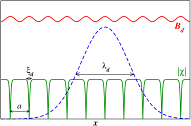
Figure 1: (Color online) A schematic plot of the spatial variation of the order parameter $\chi$ and the field $B_{d}$ in the dual Abrikosov vortex lattice. $\xi_{d}$ and $\lambda_{d}$ denote the dual coherence length and dual penetration depth, respectively. Dashed line represents the magnetic field $b_{d}({\bf r})$ associated with a single isolated vortex; $B_{d}$ in a dense lattice is a superposition of such field profiles centered at individual vortices.

We are interested in the interaction between vortices which we regard as point particles located at the phase singularities associated with each vortex. We consider a static configuration of vortices located at points ${\bf r}_{i}$ and neglect fluctuations in both $\chi$ and $A_{d}$. This corresponds to a dual mean field approximation. We emphasize that this is a highly nontrivial mean field theory since it describes the original superconductor in the presence of strong quantum fluctuations. From Eq. (15) the energy of a collection of static vortices becomes

$$E_{\rm MF}={\hbar c\over 2}\int d^{2}r\left[|(\nabla-2\pi i{\bf A}_{d})\chi|^{2}+K_{0}^{-1}(\nabla\times{\bf A}_{d})^{2}\right],$$ (18)

where, for simplicity of notation, we regard ${\bf A}_{d}$ as a 3-dimensional vector with $z$ component always zero. We have also passed back to conventional units reversing the scaling introduced in connection with Eq.(4).

The interaction energy is easiest to evaluate in the dual London approximation, where we assume a constant amplitude of the order parameter $|\chi({\bf r})|=\chi_{0}$, but arbitrary variation in its phase $\alpha$. As in the case of ordinary superconductors the London approximation is valid when the intervortex distance $a\gg\xi_{d}$ the dual coherence length; i.e. the vortex cores do not overlap. $\xi_{d}$ is difficult to estimate reliably since it depends on ${\cal V}$ in Eq. (15) which has been essentially added by hand to account for the short-distance behavior of (real) vortices. We shall assume that $\xi_{d}$ is of the order of ionic lattice spacing deep in the dual superconducting phase. Close to the transition it diverges (as $\sim\chi_{0}^{-1}$ in the mean field theory) and thus we expect the London approximation to break down in this limit.

To find the minimum of the energy we regard $E_{\rm MF}$ as a functional of ${\bf A}_{d}$ and $\alpha$ and vary it with respect to the gauge field

$${\delta E_{\rm MF}\over\delta A_{d}}=0,$$ (19)

with result

$$2\pi\chi_{0}^{2}(\nabla\alpha-2\pi{\bf A}_{d})=K_{0}^{-1}\nabla\times{\bf B}_{d}.$$ (20)

Now we can rewrite the energy as

$$E_{\rm MF}={\hbar c\over 2K_{0}}\int d^{2}r[\lambda_{d}^{2}(\nabla\times{\bf B}_{d})^{2}+{\bf B}_{d}^{2}]$$ (21)

where

$$\lambda_{d}^{2}={1\over 4\pi^{2}\chi_{0}^{2}K_{0}}.$$ (22)

$\lambda_{d}$ is the dual penetration depth which in the context of the Abrikosov lattice characterizes the magnetic size of a vortex. In the direct picture it represents the size of the charge cloud associated with a single Cooper pair.

If we apply the curl operation to Eq. (20) we obtain the dual London equation

$$-\lambda_{d}^{2}\nabla^{2}{\bf B}_{d}+{\bf B}_{d}=\hat{z}n({\bf r})$$ (23)

where

$$n({\bf r})=\sum_{i}\delta({\bf r}-{\bf r}_{i})$$ (24)

is the vortex density. The delta functions appear due to multiple valuedness of the phase in the presence of vortices; $\nabla\times\nabla\alpha({\bf r})=2\pi\hat{z}\sum_{i}\delta({\bf r}-{\bf r}_{i})$. It is clear that ${\bf B}_{d}=\hat{z}B_{d}$. The solution of the London equation (23) can be written as

$$B_{d}({\bf r})=\int d^{2}r^{\prime}G({\bf r}-{\bf r}^{\prime})n({\bf r}^{\prime}),$$ (25)

where $G({\bf r})$ is a Green’s function subject to

$$(1-\lambda_{d}^{2}\nabla^{2})G({\bf r})=\delta({\bf r}).$$ (26)

The above equation has a simple solution in the Fourier space,

$$G({\bf k})={1\over 1+\lambda_{d}^{2}k^{2}}.$$ (27)

Using a vector identity $(\nabla\times{\bf B}_{d})^{2}={\bf B}_{d}\cdot(\nabla\times\nabla\times{\bf B}_{d})+\nabla\cdot({\bf B}_{d}\times\nabla\times{\bf B}_{d})$ and discarding the vanishing surface term we rewrite the vortex energy (21) as

$$E_{\rm MF}={\hbar c\over 2K_{0}}\int d^{2}r{\bf B}_{d}\cdot[-\lambda_{d}^{2}\nabla^{2}{\bf B}_{d}+{\bf B}_{d}].$$ (28)

With the help of Eqs. (23) and (25), this can be recast as a density-density interaction

$$E_{\rm MF}={1\over 2}\int d^{2}r\int d^{2}r^{\prime}n({\bf r})V({\bf r}-{\bf r}^{\prime})n({\bf r}^{\prime}),$$ (29)

where we have introduced the intervortex potential $V({\bf r})=(\hbar c/K_{0})G({\bf r})$. In view of Eq. (24) one can also write this as interaction between point-like particles located at ${\bf r}_{i}$,

$$E_{\rm MF}={1\over 2}\sum_{ij}V({\bf r}_{i}-{\bf r}_{j}).$$ (30)

For future reference it is useful to give the intervortex potential in terms of physically accessible quantities. Specifically, we can trade compressibility $K_{0}/\hbar c$ for the Thomas-Fermi screening length $\lambda_{TF}$. In conventional terms the latter is given byam

$${1\over\lambda_{TF}^{2}}=4\pi e^{2}{1\over d}{\partial n_{0}\over\partial\mu}$$ (31)

where $n_{0}$ is the two dimensional density of particles and we have added the factor of $1/d$ to account for the layer thickness. We thus have $\hbar c/K_{0}=4\pi e^{2}\lambda_{TF}^{2}/d$. This allows us to write an explicit expression for the intervortex potential in the Fourier space as

$$V({\bf k})={e_{r}^{2}\over{\bf k}^{2}+\lambda_{d}^{-2}},$$ (32)

with the effective charge

$$e_{r}^{2}={4\pi e^{2}\over d}\left({\lambda_{TF}\over\lambda_{d}}\right)^{2}.$$ (33)

Two remarks are in order. First, despite its appearance $V({\bf r})$ is not electrostatic in origin; $e^{2}$ appears simply because we chose to express compressibility in terms of the Thomas-Fermi screening length. The interaction is mediated by phase fluctuations in the physical superconductor. Second, it is useful to consider the interaction in real space. One obtains $V({\bf r})=(e_{r}^{2}/2\pi)k_{0}(r/\lambda_{d})$ where $k_{0}(x)$ is the Hankel function of 0-th order. Of interest is its asymptotic behavior,

$$V({\bf r})={e_{r}^{2}\over 2\pi}\Biggl{\{}\begin{array}[]{ll}\left({\pi\over 2}{r\over\lambda_{d}}\right)^{1/2}e^{-r/\lambda_{d}},&r\gg\lambda_{d}\\ \ln\left({r\over\lambda_{d}}\right)+0.12,&r\ll\lambda_{d}\\ \end{array}$$ (34)

Thus the interaction has a finite range, of the order of the dual penetration depth. Approaching the transition, $\lambda_{d}$ diverges. The long distance behavior of $V$ indicates that in this limit the interaction becomes long ranged but, at the same time, its strength vanishes since $e_{r}\to 0$.

IV Normal modes in a Cooper pair Wigner crystal

The problem of normal modes in a lattice with long range Coulomb interaction has been studied previously in the context of electronic Wigner crystals.EWigner In two dimensions, vibrations of a square lattice with centrally symmetric interactions between electrons contain modes with imaginary frequencies indicating that the lattice is, in general, unstable. In the dual picture this corresponds to the well known fact that while the triangular Abrikosov vortex lattice is stable, the square lattice represents an energy maximum and is, therefore, unstable.kleiner It is also known that the square vortex lattice can be stabilized if the interactions posses four-fold anisotropy.berlinsky1 Such anisotropies can arise from the $d$-wave symmetry of the order parameter affleck or from band structure effects associated with the underlying ionic lattice.kogan1 In the following we shall make an assumption that similar terms with four-fold anisotropy exist in our dual superconductor. These terms will stabilize the square vortex lattice but will not affect our discussion of the long wavelength vibrational modes.

We employ the standard formalism for lattice vibrations: we assume that vortices are located at points ${\bf r}_{i}={\bf R}_{i}+{\bf u}_{i}$ where ${\bf R}_{i}$ denotes vectors of a Bravais lattice and ${\bf u}_{i}$ are small displacements. The interaction potential (30) is expanded to second order in the displacements,

$$V({\bf R}_{ij}+{\bf u}_{ij})\simeq V({\bf R}_{ij})+u_{ij}^{\alpha}D^{\alpha\beta}_{ij}u_{ij}^{\beta},$$ (35)

where ${\bf R}_{ij}={\bf R}_{i}-{\bf R}_{j}$, ${\bf u}_{ij}={\bf u}_{i}-{\bf u}_{j}$ and

$$D_{ij}^{\alpha\beta} = {\partial^{2}V({\bf R}_{ij}+{\bf u})\over\partial u^{\alpha}\partial u^{\beta}}\bigg{|}_{{\bf u}=0}$$ (36)

$$= -e_{r}^{2}\int{d^{2}k\over(2\pi)^{2}}{k_{\alpha}k_{\beta}\over{\bf k}^{2}+\lambda_{d}^{-2}}e^{i{\bf k}\cdot{\bf R}_{ij}}$$

is the dynamical matrix. Aside from a constant $V_{0}=\sum_{ij}V({\bf R}_{ij})$, the elastic energy can be written as

$$\Delta E=2e_{r}^{2}(I_{1}-I_{2})$$ (37)

with

$$I_{1} = \sum_{i}u_{i}^{\alpha}u_{i}^{\beta}\sum_{j}D^{\alpha\beta}_{ij},$$ (38)

$$I_{2} = \sum_{ij}u_{i}^{\alpha}u_{j}^{\beta}D^{\alpha\beta}_{ij}.$$ (39)

Note that the intervortex potential $V$ is defined everywhere in space (not only on the lattice sites) and therefore ${\bf k}$ is not restricted to the first Brillouin zone. In order to keep all momentum integration variables within the Brillouin zone we replace ${\bf k}\to{\bf q}+{\bf Q}$, and

$$\int{d^{2}k}\to\sum_{{\bf Q}}\int_{\rm BZ}{d^{2}q}\\$$ (40)

where ${\bf Q}$ is a reciprocal lattice vector ($e^{{\bf Q}\cdot{\bf R}}=1$ for any lattice vector ${\bf R}$).

We now analyze the terms $I_{1}$ and $I_{2}$ by Fourier transforming the variables ${\bf u}_{i}$,

$${\bf u}_{i}=a^{2}\int_{\rm BZ}{d^{2}k\over(2\pi)^{2}}e^{i{\bf k}\cdot{\bf R}_{i}}{\bf u}_{{\bf k}}.$$ (41)

The momentum integral is over the first Brillouin zone and $a$ is the vortex lattice constant which we include in order for ${\bf u}_{\bf k}$ to maintain the dimension of length. Combining equations (36-41) we find

$$I_{n} = -\int(d{\bf k})(d{\bf k}^{\prime})(d{\bf q})u_{\bf k}^{\alpha}u_{{\bf k}^{\prime}}^{\beta}\sum_{{\bf Q}}{(q_{\alpha}+Q_{\alpha})(q_{\beta}+Q_{\beta})\over({\bf q}+{\bf Q})^{2}+\lambda_{d}^{-2}}$$ (42)

$$\times a^{4}\sum_{ij}\begin{cases}e^{-i({\bf k}+{\bf k}^{\prime})\cdot{\bf R}_{i}+{\bf q}\cdot({\bf R}_{i}-{\bf R}_{j})}&n=1\\ e^{-i{\bf k}\cdot{\bf R}_{i}-i{\bf k}^{\prime}\cdot{\bf R}_{j}+{\bf q}\cdot({\bf R}_{i}-{\bf R}_{j})}&n=2\end{cases}$$

where $(d{\bf k})=d^{2}k/(2\pi)^{2}$ and the integration extends over the first Brillouin zone. Performing the real space sums leads to

$$\Delta E=2e_{r}^{2}\int(d{\bf k})u_{\bf k}^{\alpha}u_{-{\bf k}}^{\beta}Z_{\alpha\beta}({\bf k}),$$ (43)

with

$$Z_{\alpha\beta}({\bf k})=\sum_{{\bf Q}}\left[{(k_{\alpha}+Q_{\alpha})(k_{\beta}+Q_{\beta})\over({\bf k}+{\bf Q})^{2}+\lambda_{d}^{-2}}-{Q_{\alpha}Q_{\beta}\over Q^{2}+\lambda_{d}^{-2}}\right].$$ (44)

The normal modes of the system are related to the eigenvalues $z_{i}({\bf k})$ of the matrix $Z_{\alpha\beta}({\bf k})$. Explicitly $m_{v}\omega_{i}^{2}=2e_{r}^{2}z_{i}({\bf k})$ where $m_{v}$ is the dual vortex mass. We thus need to evaluate the reciprocal lattice sums indicated in Eq. (44). These sums are slowly convergent and great care must be taken in evaluating them; specifically we need to employ the Ewald summation technique. The following derivation is similar to that given by FetterFetter which was done in the context of a triangular Abrikosov vortex lattice.

In order to proceed analytically we split $Z_{\alpha\beta}({\bf k})=Z^{(1)}_{\alpha\beta}({\bf k})+Z^{(2)}_{\alpha\beta}({\bf k})$ with

$$Z^{(1)}_{\alpha\beta}({\bf k})={k_{\alpha}k_{\beta}\over{\bf k}^{2}+\lambda_{d}^{-2}}$$ (45)

and $Z^{(2)}_{\alpha\beta}({\bf k})$ containing the sum over all ${\bf Q}\neq 0$. Evaluation of the latter is greatly simplified if we assume that $\lambda_{d}^{-1}$ is much smaller than the smallest reciprocal lattice vector, $Q_{0}\simeq 2\pi/a$. Our estimate of $\lambda_{d}$ below will justify this assumption. Thus,

$$Z_{\alpha\beta}^{(2)}({\bf k})\approx\sum_{{\bf Q}\neq 0}\left[{(k_{\alpha}+Q_{\alpha})(k_{\beta}+Q_{\beta})\over({\bf k}+{\bf Q})^{2}}-{Q_{\alpha}Q_{\beta}\over{\bf Q}^{2}}\right].$$ (46)

We note that all the dependence on $\lambda_{d}$ is contained in $Z^{(1)}_{\alpha\beta}({\bf k})$ which is, in addition, independent of the lattice structure. $Z^{(2)}_{\alpha\beta}({\bf k})$, on the other hand, depends on the lattice structure but is independent of $\lambda_{d}$.

The detailed calculation of $Z^{(2)}_{\alpha\beta}({\bf k})$ is given in the appendix. The result can be summarized as

$$Z_{\alpha\beta}({\bf k})={k_{\alpha}k_{\beta}\over k^{2}+\lambda_{d}^{-2}}+{\vartheta\over 2}a^{2}(\delta_{\alpha\beta}k^{2}-2k_{\alpha}k_{\beta})$$ (47)

where for the square lattice $\vartheta=0.066$. Eq. (47) is valid for long wavelengths, $k\ll 2\pi/a$.

The normal modes are readily found through the eigenvalues of the matrix $Z_{\alpha\beta}({\bf k})$,

$$\omega_{1}({\bf k}) = v_{s}k,$$ (48)

$$\omega_{2}({\bf k}) = v_{s}k\sqrt{{2\over\vartheta a^{2}}{1\over k^{2}+\lambda_{d}^{-2}}-1},$$ (49)

where

$$v_{s}^{2}=\vartheta{e_{r}^{2}\over m_{v}}.$$ (50)

The first, acoustic mode, is transverse and its sound velocity is $v_{s}$. The second mode is longitudinal. At long wavelengths, $k\ll\lambda_{d}$, the longitudinal mode is also acoustic with velocity $v_{s}(\lambda_{d}/a)\sqrt{2/\vartheta}$. As the intervortex interaction becomes long-ranged ($\lambda_{d}\to\infty$) the latter speed diverges and the mode becomes gapped, which is expected on general grounds. With the estimated $\lambda_{d}$ of about 10 vortex lattice constants the longitudinal mode is unimportant (as we shall see it is the inverse of the sound velocity that enters the expressions for the specific heat and thermal conductivity). Also, had we retained the long-range Coulomb interaction mediated by the electromagnetic gauge field fluctuations, the longitudinal mode would be gapped for any value of $\lambda_{d}$. A schematic plot of the two modes is given in Fig. 2.

Figure 2: A schematic plot of the acoustic transverse mode (dashed) and the longitudinal mode (solid). The functions are plotted with $\lambda_{d}=10a$ where $a$ is the vortex lattice constant and $\omega(k)$ is presented in units of $v_{s}$.

.

V Dual vortex mass

In order to evaluate the sound velocity of the transverse acoustic mode it is essential to estimate the mass of the dual vortex. Naively this mass is simply the Cooper pair mass, $2m_{e}$. However, this is not the parameter $m_{v}$ that enters the sound velocity expression. The difference between the two originates from our scheme of calculating the normal modes. We have modeled the PWC as a system of point masses and springs. This analogy is useful but not quite suitable for the case of Cooper pairs that are delocalized over many lattice sites. The finite size of the Cooper pairs causes significant overlap between their wave functions and this leads to a situation that is quite different from the familiar case of vibrations of point-like ions in a solid.

To make these considerations more concrete let us now estimate the effective Cooper pair size given by the dual penetration depth $\lambda_{d}$. According to the STM experiments the charge modulation amounts to $\nu=1-5$% of the total charge density.Davis In a dual vortex lattice this corresponds to the rms amplitude variation of the dual magnetic field $\nu\approx\langle(B_{d}-\bar{B}_{d})^{2}\rangle^{1/2}/\bar{B}_{d}$, where $\bar{B}_{d}$ is the average field and the angular brackets denote the spatial average. The above rms variation depends on the ratio of $\lambda_{d}$ to intervortex spacing $a$.amin Namely, $a^{2}/\lambda_{d}^{2}\approx\nu$, which leads to the estimate

$$\lambda_{d}\approx(5-10)a.$$ (51)

Near half filling we can estimate $a\approx\sqrt{2}a_{0}\approx 5$Å , where the ionic lattice constant $a_{0}=3.8$Å  in YBCO. Thus, even deep in the dual superconducting phase, the charge and mass of the Cooper pair are distributed over many lattice sites.

In the present case it is intuitively clear that only the fraction of the Cooper pair mass associated with the pair density wave should contribute to the vibrational degrees of freedom. In particular as $\lambda_{d}\to\infty$ the charge distribution becomes homogeneous, the system is superfluid and cannot support any transverse modes. We thus seek a mass parameter associated with the kinetic energy of a moving dual vortex. The appropriate parameter is the inertial mass of a dual vortex. In order to determine the latter we note that, if we discard the coupling to electromagnetic field, the vortex dynamics are given by a relativistic theory Eq. (15). Correspondingly, the rest energy of a dual vortex is given by

$$E_{\rm rest}=m_{v}c_{d}^{2}.$$ (52)

Here, $m_{v}$ is the inertial mass of the dual vortex that we seek and $c_{d}$ is the dual speed of light, i.e., the phase velocity of the dual gauge field defined in Eq. (5). We may therefore estimate the energy of a vortex line $E_{\rm rest}$ in the standard wayTinkham and deduce its inertial mass through Eq. (52).

We consider a single vortex located at the origin. Its energy can be expressed by combining Eq. (28) with the dual London equation (23) and $n({\bf r})=\delta({\bf r})$ as

$$E_{\rm rest}={\hbar c\over 2K_{0}}b_{d}(0).$$ (53)

Henceforth we shall denote magnetic field associated with a single isolated vortex by $b_{d}({\bf r})$. The energy of a vortex depends linearly on the magnetic field at its center. For a circularly symmetric vortex the London equation can be solved by the Hankel function

$$b_{d}(r)={1\over 2\pi\lambda_{d}^{2}}k_{0}\left({r\over\lambda_{d}}\right)\approx{1\over 2\pi\lambda_{d}^{2}}\left[\ln\left({\lambda_{d}\over r}\right)+0.12\right]$$ (54)

where the last equality holds for $r\ll\lambda_{d}$. The divergence as $r\to 0$ is unphysical and occurs due to our neglect of the order parameter amplitude variation in the vortex core. A reliable estimate is obtained by evaluating

$$b_{d}(0)\approx b_{d}(\xi_{d})\approx{1\over 2\pi\lambda_{d}^{2}}\ln(\kappa_{d})$$ (55)

where $\kappa_{d}=\lambda_{d}/\xi_{d}$ is the dual Ginzburg-Landau parameter. $\kappa_{d}$ is assumed larger than unity (dual type-II regime) but since it appears inside the logarithm its exact value is unimportant.

The dual vortex mass is thus given by

$$m_{v}={\hbar\over 4\pi c\lambda_{d}^{2}K_{1}}\ln(\kappa_{d})={4e^{2}\over dc^{2}}\left({\lambda\over\lambda_{d}}\right)^{2}\ln(\kappa_{d}).$$ (56)

We have used the London penetration depth,

$$\lambda^{-2}={4\pi e^{2}n_{s}\over m_{e}c^{2}}$$ (57)

with the superfluid density $n_{s}=2\Psi_{0}^{2}/d$ to eliminate $K_{1}=\hbar\Psi_{0}^{2}/2m_{e}c$. In the above estimate one should take the mean field value of $\lambda$, i.e. the value it would have in the absence of phase fluctuations. In YBCO, we thus take $\lambda\simeq 1000$Å, the value at optimum doping. Taking $\kappa_{d}=10$ and $d=12$Å  gives $m_{v}\simeq 1.1\times 10^{-5}(\lambda/\lambda_{d})^{2}(2m_{e})$, where $m_{e}$ is the electron mass.

A more instructive way of expressing $m_{v}$ is to estimate the mean field superfluid density close to half filling by $n_{s}\approx 1/(2a_{0}^{2}d)$ and obtain

$$m_{v}=2m_{e}\left({a_{0}\over\lambda_{d}}\right)^{2}{\ln(\kappa_{d})\over 2\pi}.$$ (58)

As expected, when Cooper pairs are localized and $\lambda_{d}$ approaches the lattice constant $a_{0}$ the inertial mass of the dual vortex approaches that of the Cooper pair. When, on the other hand, $\lambda_{d}\gg a_{0}$, the Cooper pair is delocalized over many lattice spacings and the dual vortex mass becomes small.

VI Interlayer tunneling and dual monopoles

A linear dispersion such as the one we found for the transverse mode, combined with Bose-Einstein distribution for phonons, leads to specific heat $C_{v}\sim T^{d}$ where $d$ is the dimensionality of the system. The thermal conductivity, within the simple Boltzmann approach, is $\kappa={1\over 3}C_{v}v_{s}\ell$ where $\ell$ denotes the phonon mean free path. Assuming the latter is $T$-independent, as is the case for phonons scattered by the sample boundaries, we have $\kappa\sim T^{d}$. We thus arrive at a conclusion that, in order to agree with experiment, the PWC phonons must propagate in all 3 dimensions.

Our theory thus far focused on purely two dimensional physics of the Cu-O layers. However, it is clear that vibrations of PWC in the adjacent layers will be coupled. There are two main sources of this coupling: (i) the pair tunneling between the layers represented by the interlayer Josephson term and (ii) the Coulomb interaction between the induced charge modulations. Inclusion of the interlayer coupling will cause the PWC phonons to propagate between the layers. To complete our calculation we must determine the associated sound velocity in the $\hat{z}$ direction.

Ideally, we would like to extend our duality map to a system of weakly coupled layers and repeat the calculation of the normal modes. Unfortunately, there is no straightforward generalization of the vortex-boson duality to a system in 3+1 dimensions; 2+1 dimensional systems are special in this respect. The reason for this can be seen most clearly by returning back to Eq. (10). In (3+1)D it is not possible to enforce the zero-divergence constraint on $W_{\mu}$ by expressing it as a curl of a gauge field; the curl operation is only meaningful in 3 dimensions. On a more fundamental level in (3+1)D vortices cannot be regarded as point particles, rather they should be thought of as strings. Thus, rather than a dual superconductor, in (3+1)D the duality map produces a string theory. On physical grounds we still expect the PWC to form in a (3+1)D phase disordered superconductor but the underlying mathematical structure of the dual theory appears to be more complicated and beyond the scope of this paper.remark1 ; strings

We thus continue describing the physics of the individual layers by the (2+1)D duality and consider the effect of weak interlayer coupling on the resulting quantum state. We focus first on the Josephson coupling, which mediates tunneling of Cooper pairs between layers. Formally we imagine generalizing our starting Lagrangian (2) into a Lawrence-Doniach modelTinkham ; doniach1 for a multilayer system by attaching a layer index $m$ to the scalar field $\Psi$ and adding a term

$${J_{0}\over 2a_{0}^{2}}|\Psi_{m}-\Psi_{m+1}|^{2}$$ (59)

to couple the layers. The cross terms describe tunneling of physical Cooper pairs between the layers. The amplitude for this process, $J_{0}$, is related to the $c$-axis London penetration depth $\lambda_{c}$ by

$$J_{0}={a^{2}_{0}\over d}{\hbar^{2}c^{2}\over 16\pi e^{2}\lambda_{c}^{2}}.$$ (60)

From the point of view of an individual layer removal of a Cooper pair represents a monopole event. A tunneling event occurring at a particular instant of imaginary time adds or removes a Cooper pair from the plane. In the dual description, this event corresponds to the appearance or disappearance of a vortex; the magnetic flux lines associated with it originate or terminate at the same point, as illustrated in Fig.3a. A point in space-time which represents a drain (source) of a magnetic flux is known as magnetic monopole (antimonopole). The vortex must reappear in the adjacent layer and this corresponds to an antimonopole. In ordinary superconductors vorticity is strictly conserved which can be regarded as a consequence of the absence of monopoles in the real world. In the dual superconductor vorticity is conserved only if we consider a system with fixed number of Cooper pairs. Once we introduce the Josephson tunneling vorticity is conserved only globally (i.e. the total number of vortices in all layers is constant) and we must permit monopole-antimonopole pairs to occur in the adjacent layers.

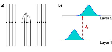
Figure 3: (Color online) a) A schematic illustration of the flux lines in the presence of a monopole. b) Josephson tunneling with lateral displacement of the dual vortex. The shaded regions represent charge densities associated with a Cooper pair in the PWC.

.

To model the interlayer tunneling we should thus regard the dual gauge field $A_{d}$ as compact and append to the dual Lagrangian (15) a term describing monopole-antimonopole events occurring in the adjacent layers. Since, ultimately, we only need the mean field description of the intervortex interaction, we shall adopt a simpler and physically more intuitive approach. In essence, all we need to complete our description of PWC vibrations is an effective potential, akin to $V({\bf r}_{i}-{\bf r}_{j})$, that will describe the coupling between vortices in adjacent layers induced by the Josephson tunneling. Taking our clue from Eq. (30) we describe the system with many layers by a Hamiltonian $H=H_{0}+H_{J}$ with

$$H_{0} = {1\over 2}\sum_{m}\int_{\bf r}\int_{{\bf r}^{\prime}}\psi^{\dagger}_{m}({\bf r})\psi^{\dagger}_{m}({\bf r}^{\prime})V({\bf r}-{\bf r}^{\prime})\psi_{m}({\bf r}^{\prime})\psi_{m}({\bf r}),$$

$$H_{J} = \sum_{m}\int_{\bf r}\int_{{\bf r}^{\prime}}J({\bf r}-{\bf r}^{\prime})[\psi^{\dagger}_{m}({\bf r})\psi_{m+1}({\bf r}^{\prime})+{\rm h.c.}],$$ (61)

The operator $\psi^{\dagger}_{m}({\bf r})$ creates a vortex at point ${\bf r}$ in the $m$-th layer and $\int_{\bf r}=\int d^{2}r$. $H_{0}$ describes interactions between vortices within a layer and $H_{J}$ generates the Josephson coupling; $J$ is the amplitude for interlayer tunneling to be discussed shortly. For now we regard vortices as infinitely heavy (no kinetic energy in the plane).

Our strategy will be to treat $H_{J}$ as a small perturbation on the eigenstates of $H_{0}$. This is justified as long as $J$ is very small. In the limit of infinite mass the unperturbed eigenstates are labeled by the positions $\{{\bf r}_{im}\}$ of $N$ individual vortices within each layer. The energy of this state is simply given by Eq. (30). Clearly, there will be no correction to the energy to first order in $H_{J}$. The leading contribution appears in second order and describes a virtual hop of a Cooper pair from one layer to the next and then back. For simplicity we consider a case of two layers, $m=1,2$, and evaluate the second order correction to the energy from such processes:

$$\Delta E^{(2)}=\sum_{\eta=\pm 1}\int_{\bf s}\int_{{\bf s}^{\prime}}{|\langle N,N|H_{J}|N+\eta_{\bf s},N-\eta_{{\bf s}^{\prime}}\rangle|^{2}\over E(N,N)-E(N+\eta_{\bf s},N-\eta_{{\bf s}^{\prime}})}.$$ (62)

In an obvious notation $|N,N\rangle$ denotes a state with $N$ pairs in each layer, located at $\{{\bf r}_{i1}\}$ and $\{{\bf r}_{i2}\}$, while $|N+\eta_{\bf s},N-\eta_{{\bf s}^{\prime}}\rangle$ represents a state with one pair added (removed) at ${\bf s}$ in layer 1, and one pair removed (added) at ${\bf s}^{\prime}$ in layer 2, for $\eta=1(-1)$.

The matrix element in the numerator is easily seen to be just $|J({\bf s}-{\bf s}^{\prime})|^{2}$ but the energy denominator requires some careful thought. An obvious contribution to the energy difference comes from the interaction between Cooper pairs expressed through Eq. (30). For $\eta=+1$ this is simply the interaction energy of a vortex added at ${\bf s}$ in layer 1 and antivortex added at ${\bf s}^{\prime}$ in layer 2,

$$\Delta U=-\sum_{i}[V({\bf s}-{\bf r}_{i1})-V({\bf s}^{\prime}-{\bf r}_{i2})].$$ (63)

For $\eta=-1$ the overall sign is reversed. However, this cannot be the whole story since Eq. (63) does not account for the fact that the state with $N$ vortices per layer corresponds to the absolute minimum of the total energy of the unperturbed system. At the level of Eq. (30) this requirement is implemented as a constraint. This is adequate as long as $N$ is held constant. Once we allow for number fluctuations, however, we must consider the energy cost $U_{0}$ of removing (adding) a Cooper pair from (to) a layer. Ultimately, this cost is related to the electric charge neutrality: removing or adding a pair from/to a neutral layer costs Coulomb energy. Thus, we estimate $U_{0}$ as the electrostatic energy of the charge distribution corresponding to an extra pair at ${\bf s}$ in layer 1 and a missing pair at ${\bf s}^{\prime}$ in layer 2. The missing pair is modeled simply as an effective positive charge distribution on the otherwise neutral background. We have

$$U_{0}={1\over 2\epsilon}\int_{\bf R}\int_{{\bf R}^{\prime}}{\rho({\bf R})\rho({\bf R}^{\prime})\over|{\bf R}-{\bf R}^{\prime}|},$$ (64)

with ${\bf R}=({\bf r},z)$ a three dimensional vector. $\epsilon$ is the dielectric constant which reflects the polarizability of the insulating medium between the Cu-O layers. Its value is around 10 in YBCO.tsvetkov Taking

$$\rho({\bf R})=\rho_{1}({\bf r}-{\bf s})\delta(z)-\rho_{1}({\bf r}-{\bf s}^{\prime})\delta(z-d),$$ (65)

where $\rho_{1}({\bf r})=(2e)b_{d}({\bf r})$ is the planar charge density associated with a single Cooper pair in PWC, we obtain

$$U_{0}={(2e)^{2}\over\epsilon}\int_{\bf r}\int_{{\bf r}^{\prime}}b_{d}({\bf r})b_{d}({\bf r}^{\prime})\left[{1\over|{\bf r}-{\bf r}^{\prime}|}-{1\over\sqrt{({\bf r}-{\bf r}^{\prime}-{\bf l})^{2}+d^{2}}}\right],$$ (66)

with ${\bf l}={\bf s}-{\bf s}^{\prime}$. For general values of ${\bf l}$ and $d$ the above integral must be evaluated numerically. However, it turns out that we shall only require its leading behavior in the limit $d,|{\bf l}|\ll\lambda_{d}$, i.e. the situation when the distance between the two charge clouds is small compared to their lateral size given by $\lambda_{d}$. In this limit we can expand

$$U_{0}\simeq{(2e)^{2}\over\lambda_{d}\epsilon}\left[{d\over 2\lambda_{d}}+{\pi\over 8}{{\bf l}^{2}\over\lambda_{d}^{2}}\right].$$ (67)

The energy correction (62) thus becomes

$$\Delta E^{(2)}=-\int_{\bf s}\int_{{\bf s}^{\prime}}\left[{J^{2}\over U_{0}+\Delta U}+{J^{2}\over U_{0}-\Delta U}\right]$$ (68)

where we have suppressed various arguments in order to display the structure of the result. We notice that $\Delta E^{(2)}$ depends on the positions $\{{\bf r}_{i1}\}$ and $\{{\bf r}_{i2}\}$ through $\Delta U$. Upon integration over ${\bf s},{\bf s}^{\prime}$ this will produce interactions between vortices in different layers, as expected. The origin of this interaction lies in the fact that the energy of the virtual intermediate state depends on the position of the extra Cooper pair relative to the pairs already present in that layer. Since the positions of the former before and after the tunneling event are strongly correlated this induces interaction between Cooper pairs in the adjacent layers.

We can make the form of the interlayer interaction more explicit in the limit $|\Delta U|\ll U_{0}$ by expanding

$$\Delta E^{(2)}\simeq-\int_{\bf s}\int_{{\bf s}^{\prime}}{2J^{2}\over U_{0}}\left[1+\left({\Delta U\over U_{0}}\right)^{2}+{\cal O}\left({\Delta U\over U_{0}}\right)^{4}\right].$$ (69)

The first term is a constant, but the second term, when expanded with help of Eq. (63), contains the following expression,

$$V_{z}({\bf r}_{i1}-{\bf r}_{j2})=4\int_{\bf s}\int_{{\bf s}^{\prime}}V({\bf r}_{i1}-{\bf s}){|J({\bf s}-{\bf s}^{\prime})|^{2}\over U_{0}^{3}({\bf s}-{\bf s}^{\prime})}V({\bf s}^{\prime}-{\bf r}_{j2})$$ (70)

which provides an explicit interaction potential between the pairs located in the adjacent layers. Although we derived Eq. (70) assuming just two layers it is obvious that it generalizes to a multilayer system.

In order to complete our computation of $V_{z}$ we must determine the form of the tunneling matrix element $J({\bf s}-{\bf s}^{\prime})$. In the direct picture, modeled by a Lawrence-Doniach type Hamiltonian,doniach1 Cooper pairs are assumed to tunnel ‘straight up’ (or down), i.e. from a point ${\bf s}$ in one layer to the point ${\bf s}$ in the adjacent layer. A subtlety in the dual picture arises from the fact that $H_{J}$ describes tunneling of dual vortex cores and not Cooper pairs directly. We recall that even when the position of the dual vortex is sharply localized at a point ${\bf s}$, the associated Cooper pair charge (and number) density is delocalized over the length scale $\lambda_{d}$ around ${\bf s}$ with the probability density given by $b_{d}({\bf r}-{\bf s})$. Thus, we can think of a Cooper pair as being described by a wave function whose envelope varies as $\sqrt{b_{d}({\bf r}-{\bf s})}$. As illustrated in Fig. 3.b a straight up tunneling of a Cooper pair in general may lead to dual vortex core tunneling with nonzero lateral displacement. The associated amplitude to tunnel from point ${\bf s}$ to ${\bf s}^{\prime}$ will be given by the overlap of the two pair wave functions, $\sim\int_{\bf r}\sqrt{b_{d}({\bf s}-{\bf r})b_{d}({\bf r}-{\bf s}^{\prime})}$. This last integral is somewhat difficult to evaluate because of the square root, but the resulting function is clearly close to $b_{d}({\bf s}-{\bf s}^{\prime})$. In the following we thus use

$$J({\bf r})\approx J_{0}b_{d}({\bf r}),$$ (71)

which turns out to be properly normalized since $\int_{\bf r}b_{d}({\bf r})=1$.

An important implication of the above result (71) is that tunneling over lateral distances larger than $\lambda_{d}$ is exponentially suppressed and we may indeed use the approximation (67) for $U_{0}$ when evaluating $V_{z}$ from Eq. (70). In fact we will use only the first term in (67) which gives the leading contribution of the form,

$$V_{z}({\bf r})={4J_{0}^{2}e_{r}^{4}\over U_{0}^{3}}\left[\lambda_{d}^{4}\int_{\bf s}\int_{{\bf s}^{\prime}}b_{d}({\bf r}-{\bf s})b_{d}({\bf s}-{\bf s}^{\prime})^{2}b_{d}({\bf s}^{\prime})\right],$$ (72)

where we have used the relation $V({\bf r})=e_{r}^{2}\lambda_{d}^{2}b_{d}({\bf r})$ in order to express everything in terms of $b_{d}$. It is worth noting that in Eq. (72) the prefactor

$$E_{J}={4J_{0}^{2}e_{r}^{4}\over U_{0}^{3}}$$ (73)

characterizes the energy scale for the interlayer coupling while the expression in the square brackets represents a dimensionless function of spatial variable ${\bf r}$ whose range is set by $\lambda_{d}$. The interaction is repulsive.

We could now repeat the calculation of the normal modes for the layered system. This calculation,unpublished however, is lengthy and does not yield any new physical insights to the problem at hand. All we need, in fact, is the result for the speed of sound in the $\hat{z}$ direction. This can be readily estimated in analogy with Eq. (50) which states that up to a numerical constant the speed of sound squared equals the energy scale of the interaction divided by mass. This of course is a well known result for ordinary systems of springs and masses; what Eq. (50) confirms is that this result remains valid even in the case of interactions with finite range. We thus obtain

$$v_{z}^{2}\simeq{E_{J}\over m_{v}}={4J_{0}^{2}e_{r}^{4}\over U_{0}^{3}m_{v}}.$$ (74)

The above is a perturbative result and remains valid only as long as $J_{0}/U_{0}\ll 1$. With help of Eqs. (67) and (60) this condition becomes

$$1\gg{J_{0}\over U_{0}}=\left({a\over d}\right)^{2}{\epsilon\over 16\pi\alpha^{2}}\left({\lambda_{d}\over\lambda_{c}}\right)^{2}\simeq 4.1\times 10^{2}\left({\lambda_{d}\over\lambda_{c}}\right)^{2},$$ (75)

where $\alpha=e^{2}/\hbar c\simeq 1/137$ is the fine structure constant. The latter appears because the Josephson coupling connects two “dual worlds” through the real world coupling. Since $\lambda_{c}$ is typically very large in cuprates $\sim 10^{4}-10^{5}$Å  Eq. (75) should be well satisfied except very close to the transition.

We now briefly discuss the direct Coulomb interaction, which will turn out to be negligible in most cases. If we assume that only the interaction between neighboring layers is important then standard treatment leads to acoustic dispersion for the transverse mode along the $\hat{z}$ direction with the sound velocity $\sqrt{E_{C}/m_{v}}$ where $E_{C}$ is of the order of the Coulomb potential at distance $d$,

$$E_{C}={(2\nu e)^{2}\over\epsilon d}$$ (76)

Here $2\nu e\simeq 2ea^{2}/\lambda_{d}^{2}$ is the fraction of Cooper pair charge that is modulated. As mentioned above $\nu\approx(1-5)\%$ in the STM experiments.

For the typical values of various parameters listed below Eq. (82) and $\lambda_{d}=20$Å  we find $E_{J}/E_{C}\approx 30$; the Josephson term dominates. It is also important to note that $E_{J}$ and $E_{C}$ exhibit very different scaling with $\lambda_{d}$. In particular Eq. (73) implies that $E_{J}\sim\lambda_{d}^{2}$ while $E_{C}\sim\lambda_{d}^{-4}$. Thus, even if far away from the transition the direct Coulomb contribution is significant, as the transition is approached and $\lambda_{d}$ becomes large, the Josephson coupling between the layers always takes over. In the following we shall thus focus exclusively on the latter.

VII Specific heat and thermal conductivity

Having found the eigenmodes of the PWC as well as the effective mass of dual vortices, we may now combine these results and calculate the specific heat and the thermal conductivity associated with the transverse vibrational modes. As mentioned above the longitudinal modes either have much higher speed or are gapped and thus will not contribute at low temperatures.

Let us first estimate the transverse in-plane sound velocity (50) in terms of physically meaningful parameters. Combining Eqs. (33) and (56) this becomes

$$v_{s}=c\sqrt{\pi\vartheta\over\ln(\kappa_{d})}\left({\lambda_{TF}\over\lambda}\right).$$ (77)

We observe that the dependence on $\lambda_{d}$ has dropped out, except through $\kappa_{d}$. We expect Eq. (77) to be valid only deep in the PWC state; as one approaches the transition point the dual London approximation ceases to apply.

Thomas-Fermi screening length is normally of the order of inverse Fermi wave vector $k_{F}$, or several Å. The ratio of the two length scales is thus about $10^{-2}-10^{-3}$. For $\kappa_{d}\simeq 10$ the square root is 0.30. Eq. (77) thus gives $v_{s}$ about an order of magnitude smaller than the Fermi velocity in cuprates (the latter is $\sim 10^{-2}c$). This makes sense physically since the PWC vibrations are purely electronic phenomenon, and, thus, on dimensional grounds one expects $v_{s}$ and $v_{F}$ to be of similar order of magnitude.

Similarly we can express the interplane sound velocity $v_{z}$ associated with the Josephson coupling. Evaluating Eq. (74) with help of Eqs. (33), (56), (60) and (67) we obtain

$$v_{z}=c{\epsilon^{3/2}\over 8\sqrt{2\ln(\kappa_{d})}}\left({a_{0}\over d}\right)^{2}\left({\lambda_{TF}^{2}\over d\lambda}\right)\left({\lambda_{d}\over\alpha\lambda_{c}}\right)^{2}.$$ (78)

Thus, $v_{z}$ grows with $\lambda_{d}$. According to the criterion (75) the perturbation theory breaks down when $(\lambda_{d}/\lambda_{c}\alpha)$ becomes of the order of $10$. A glance at Eqs. (77) and (78) confirms that this makes sense physically for in this limit $v_{z}$ approaches $v_{s}$. The sound velocity becomes isotropic and we may no longer treat the interlayer tunneling as a perturbation.

Repeating the standard calculation of the phonon specific heat for the case of sound velocity with uniaxial anisotropy leads to

$$C_{v}={2\gamma k_{B}^{4}\over\pi^{2}\hbar^{3}v_{s}^{2}v_{z}}T^{3},$$ (79)

where $\gamma=\int_{0}^{\infty}dxx^{3}/(e^{x}-1)=\pi^{4}/15$. The associated thermal conductivity in the Cu-O plane becomes

$$\kappa={1\over 3}C_{v}v_{s}\ell=\beta T^{3},$$ (80)

with

$$\beta={2\gamma k_{B}^{4}\ell\over 3\pi^{2}\hbar^{3}v_{s}v_{z}}.$$ (81)

Combining Eqs. (77), (78) with Eq. (81) we obtain

$$\beta=(0.007-3.5)\left({10{\rm\AA}\over\lambda_{d}}\right)^{2}{\rm mW\over K^{4}cm},$$ (82)

where the lower bound obtains if we take $\lambda=1030$Å  and $\lambda_{c}=6.2\lambda$ as found for optimally doped YBCO,esr while the upper bound obtains for $\lambda=2020$Å  and $\lambda_{c}=37.7\lambda$, values relevant to the 56K “ortho-II” phase. In both cases we take $\lambda_{TF}\simeq a_{0}=3.8$Å , $d=12$Å , $\epsilon=10$ and $\kappa_{d}=10$. We assume that the phonon mean free path $\ell\simeq 0.05$mm, which is the geometric average of the width ($\sim 500\mu$m) and the thickness ($\sim 10\mu$m) of samples used in the experiment.Taillefer1

The experimental resultTaillefer1 for the point farthest from the transition gives $\beta\approx 0.5$ mW/K⁴ cm. With the value of $\lambda_{d}=25-50$Å, estimated from the STM data via Eq. (51), our result above is broadly consistent with the experimental data, although it has to be noted that it depends strongly on the assumed values of the input parameters, most notably on the $ab$-plane and $c$-axis penetration depths. These are known in YBCO with high accuracyesr but they also vary strongly with doping and it is not entirely clear which values one should adopt in the estimate of $\beta$. We have argued above that one should take the underlying mean-field, noninteracting values, which are presumably most accurately approximated by the values measured near the optimal doping. Within the class of phase fluctuation models considered here, any reduction of superfluid density upon underdoping is attributed to an interaction effect beyond mean field theory. In reality, part of the change may be associated with the change of the underlying mean-field ground state but it is impossible to make a precise statement about this. It is also possible that the measured values at optimal doping already reflect a fair amount of fluctuations and the underlying mean-field superfluid density should be higher. The range of values displayed in Eq. (82) is meant to be indicative of these various uncertainties.

VIII Summary and open issues

We have studied the normal modes of a pair Wigner crystal employing a duality transformation from a phase fluctuating superconductor to a fictitious dual type-II superconductor in applied magnetic filed. Vortices in the dual superconductor represent Cooper pairs in the original model and the vibrational modes of the PWC can be calculated as magnetophonons of the dual Abrikosov vortex lattice. Assuming that that pinning of the dual vortex lattice to the underlying ionic lattice is negligible, as suggested by the fact that PWC is incommensurate in some cases, the transverse magnetophonon is acoustic and will thus contribute to the low energy thermal and transport properties of the system. For charged systems longitudinal modes will be gapped. Our main result is the estimate of the sound velocity of the transverse mode which determines the magnitude of its contribution to the specific heat and thermal conductivity. The in-plane velocity, $v_{s}$, is found to be about an order of magnitude lower than the Fermi velocity $v_{F}$. Together with our estimate of the interplane sound velocity, $v_{z}$, which we assumed to be determined primarily by the Josephson coupling between the neighboring layers, our considerations yield a $T^{3}$ contribution to the thermal conductivity with a prefactor consistent with the recently reported bosonic mode in strongly underdoped single crystals of YBCO.Taillefer1

An important length scale in this problem is the dual penetration depth, $\lambda_{d}$, which has the physical meaning of the size of the Cooper pair in the PWC. STM experiments indicate that $\lambda_{d}$ is much larger than the distance between the Cooper pairs; the latter are extended objects with strong zero-point motion and overlapping wave functions. This is the main reason why duality is a useful concept in this problem: it provides a convenient tool for the description of a strongly quantum fluctuating system of Cooper pairs in terms of dual vortices that can be treated as point particles. The latter are local objects and their physics can be accurately described in the mean field approximation.

A key assumption, underlying all our preceding considerations and results, is that the pair Wigner crystal is essentially decoupled from the ionic lattice. As mentioned in the Introduction transverse modes of a PWC pinned to the ionic lattice would be gapped and thus irrelevant at low temperatures. The duality transformation reviewed in Sec. II shows that PWC indeed can exist in continuum, independently of any underlying crystalline lattice. There is, therefore, no logical contradiction implied by the above assumption. In the context of cuprates one must ask to what extent does the continuum model reflect the physics of Cooper pairs moving in the copper-oxygen planes. The key issue here is whether PWC is commensurate or incommensurate with the underlying ionic lattice, since incommensurate PWC cannot be pinned, except by disorder. Pinning by disorder affects the magnetophonon mean free path but in general does not open a gap in the phonon spectrum.

The problem of commensurability is a difficult one to analyze theoretically as it involves the details of PWC energetics, band structure and electron-ion interaction. Our argument in favor of the incommensurate PWC is therefore largely phenomenological and is based on the following three observations. First, the checkerboard patterns in at least some experimentsVershinin ; Hashimoto have been reported to have period clearly different from 4 ionic lattice constants (the values range between $4.2-4.7a_{0}$) implying incommensurate PWC. The mere existence of such an incommensurate PWC indicates that coupling to the lattice must be extremely weak even in the case when the PWC is commensurate. Second, the PWC appears to exist for a relatively wide range of dopings. If only commensurate PWC were allowed then one would expect dramatic changes in PWC structure upon variation of the pair density; in particular the unit cell size would vary significantly as the PWC adjusted to different doping levels. No such dramatic variations are observed. It appears, instead, that PWC structure, where it exists, is largely independent of doping. Finally, we found that Cooper pairs in a crystal proximate to a superconductor have wavefunctions delocalized over many lattice constants. We may expect that a potential with ionic lattice periodicity should be relatively ineffective in pinning such delocalized objects.

An issue which might require further consideration is the dependence of the sound velocity of the PWC on the doping level of the system. Experimentally the strength of the $T^{3}$ mode goes to zero continuously as the transition to the superconducting state is approached. In our theory the transition is marked by the divergence of the dual penetration depth $\lambda_{d}$. We found the in-plane sound velocity to be independent of $\lambda_{d}$. This is due to the exact cancellation between the strength of intervortex interaction $e_{r}$ and the dual vortex mass $m_{v}$: both vanish as $\lambda_{d}\to\infty$. The $c$-axis sound velocity is proportional to $\lambda_{d}^{2}$ which ensures that the thermal conductivity of the bosonic modes decreases as the transition is approached, in agreement with the experiment. It is important to emphasize, however, that there is no reason to expect that this result will remain valid very close to the transition. First, $v_{z}$ is obtained in a perturbation theory which is only valid as long as $\lambda_{d}/\lambda_{c}\ll 1$. Outside of this regime one must treat the full 3D system. Second, the dual London approximation also breaks down near the transition since the vortex cores begin to overlap. To address the physics of magnetophonons near the transition one would have to treat vortex vibrations in the full Ginzburg-Landau theory Eq. (18). Qualitatively we expect that the amplitude fluctuations will make the intervortex interaction stronger, leading to increase in $v_{s}$ and thus reduction of thermal conductivity as the transition is approached, in accord with experiment. Detailed calculations, however, present a daunting challenge and are left for future investigation.

Another open issue is the inclusion of the detailed structure of the PWC. We have assumed a simple square Bravais lattice of Cooper pairs. Experiments Hanaguri ; McElroy ; Hashimoto and detailed theoretical considerations Melikyan ; balents1 indicate a lattice with square symmetry, but with a more complicated internal structure. Within our approach this could be modeled as a square vortex lattice with a basis. The vibrational spectrum of such a lattice will be more complicated but will retain the acoustic mode derived above which reflects the center of mass motion of the unit cell.

STM studies also indicate the presence of domain walls and other defects in the PWC. Such defects would scatter PWC phonons and cause a short mean free path $\ell$. Our estimate, on the other hand, suggests that in YBCO $\ell$ should be of the order of the sample size. This implies that the PWC in YBCO is much more homogeneous than that in BiSCCO and Na-CCOC. Given the extreme purity of the YBCO crystals used in the thermal conductivity measurementTaillefer1 this is perhaps not surprising. Unfortunately YBCO is not amenable to high-precision STM studies due to its lack of a natural cleavage plane. It would be interesting to see if the bosonic mode could be observed in the thermal conductivity of Na-CCOC. Based on our model we would expect it to be much weaker due to much shorter mean free path $\ell$.

Acknowledgments The authors are indebted to E. Altman, J.C. Davis, T. P. Davis, N. Doiron-Leyraud, M.P.A. Fisher, K. LeHur, L. Taillefer, and Z. Tešanović for stimulating discussions and correspondence. The work has been supported in part by NSERC, CIAR, A.P. Sloan Foundation and the Aspen Center for Physics.

Appendix A Evaluation of $Z_{xy}^{\alpha\beta}$

This appendix follows the calculation of Fetter,Fetter adjusted to the case of the square lattice. The matrix $Z_{\alpha\beta}^{(2)}$ is a symmetric rank-2 tensor. In terms of the vector ${\bf k}$ it can therefore be written as

$$Z_{\alpha\beta}^{(2)}({\bf k})=A(k^{2})\delta_{\alpha\beta}+B(k^{2}){k_{\alpha}k_{\beta}\over k^{2}}$$ (83)

where $A$ and $B$ are scalar functions of $k^{2}$. The trace of $Z^{(2)}$ vanishes to first order in $1/(\lambda_{d}^{2}Q_{0}^{2})$, thus

$$2A(k^{2})+B(k^{2})=0.$$ (84)

We evaluate the off-diagonal elements of the matrix to determine $B(k^{2})$.

Let us define

$$S({\bf k})=2\pi n_{v}\sum_{Q\neq 0}\left[{(Q_{x}+k_{x})(Q_{y}+k_{y})\over({\bf Q}+{\bf k})^{2}}-{Q_{x}Q_{y}\over{\bf Q}^{2}}\right]$$ (85)

where $n_{v}={1/a^{2}}$ is the density of vortices. Ewald summation technique splits the above sum into two parts, $S=S_{d}({\bf k})+S_{r}({\bf k})$, in such a way that $S_{d}$ converges rapidly in real space while $S_{r}$ converges rapidly in reciprocal space. One obtains, for any Bravais lattice,Fetter

$$S_{d} = 2\sum_{j}(1-e^{i{\bf k}\cdot{\bf R}_{j}}){X_{j}Y_{j}\over R_{j}^{4}}(1+\pi n_{v}R_{j}^{2})e^{-\pi n_{v}R_{j}^{2}}$$

$$S_{r} = 2\pi n_{v}\sum_{{\bf Q}\neq 0}{(Q_{x}+k_{x})(Q_{y}+k_{y})\over({\bf Q}+{\bf k})^{2}}e^{-({\bf Q}+{\bf k})^{2}/4\pi n_{v}}$$ (86)

$$- 2\pi n_{v}{k_{x}k_{y}\over k^{2}}(1-e^{-k^{2}/4\pi n_{v}})$$

where ${\bf R}_{j}=(X_{j},Y_{j})$ is a lattice vector. The above sums can be easily evaluated numerically for arbitrary ${\bf k}$. For small wave vector $|k|$ we may expand $S_{d}$ and $S_{r}$ to second order

$$S_{d} \approx 2k_{x}k_{y}{\sum_{j}}^{\prime}{X_{j}^{2}Y_{j}^{2}\over R_{j}^{4}}(1+\pi n_{v}R_{j}^{2})e^{-\pi n_{v}R_{j}^{2}}$$ (87)

$$S_{r} \approx -{1\over 2}k_{x}k_{y}\left[{\sum_{Q}}^{\prime}\left(1-{Q^{2}\over 8\pi n_{v}}\right)e^{-Q^{2}/4\pi n_{v}}+1\right]$$

where $\sum^{\prime}$ denotes a summation that excludes the zero vector. In order to perform the sums for the square lattice we substitute

$${\bf R}=a(l,m),\ \ {\bf Q}={2\pi\over a}(l,m)$$ (88)

and arrive at

$$S_{d} = k_{x}k_{y}{\sum_{l,m}}^{\prime}{2l^{2}m^{2}\over(l^{2}+m^{2})^{2}}[1+\pi(l^{2}+m^{2})]e^{-\pi(l^{2}+m^{2})}$$

$$S_{r} = {1\over 2}k_{x}k_{y}\bigl{(}{\sum_{l,m}}^{\prime}[1-{\pi\over 2}(l^{2}+m^{2})]e^{-\pi(l^{2}+m^{2})}+1\bigr{)}$$

The sums over $m$ and $l$ are rapidly convergent and can be evaluated numerically. This gives the off-diagonal part of $Z^{(2)}$

$$Z^{(2)}_{xy}({\bf k})=-0.415{a^{2}\over 2\pi}k_{x}k_{y}\equiv-\vartheta a^{2}k_{x}k_{y},$$ (89)

with $\vartheta=0.066$. Thus, $B(k^{2})=-\vartheta a^{2}k^{2}$.

References

- (1) We wish to alert the reader to the well known subtlety involved in deriving the uncertainty relation for the compact phase variable; see e.g. P. Carruthers and M.M. Nieto, Phys. Rev. Lett. 14, 387 (1965). This issue, however, does not affect our subsequent discussion.
- (2) C. Dasgupta and B.I. Halperin, Phys. Rev. Lett. 47, 1556 (1981).
- (3) M.P.A. Fisher and D.H. Lee, Phys. Rev. B39, 2756 (1989).
- (4) D.R. Nelson, Phys. Rev. Lett. 60, 1973 (1988).
- (5) T. Timusk and B.W. Statt, Rep. Prog. Phys. 62, 61 (1999).
- (6) V.J. Emery and S.A. Kivelson, Nature 374, 434 (1995)
- (7) M. Randeria, Varenna Lectures (cond-mat/9710223).
- (8) M. Franz and A.J. Millis, Phys. Rev. B58, 14572 (1998).
- (9) L. Balents, M.P.A. Fisher and C. Nayak, Phys. Rev. B60, 1654 (1999).
- (10) M. Franz and Z. Tešanović, Phys. Rev. Lett. 87, 257003 (2001).
- (11) J. Corson R. Mallozzi, J. Orenstein, J. N. Eckstein, I. Bozovic, Nature 398, 221 (1999)
- (12) Z.A. Xu, N. P. Ong, Y. Wang, T. Kakeshita, S. Uchida, Nature 406, 486 (2000).
- (13) Y. Wang, L. Li, M.J. Naughton, G.D. Gu, S. Uchida and N.P. Ong, Phys. Rev. Lett. 95, 247002 (2005).
- (14) M. Sutherland, S. Y. Li, D. G. Hawthorn,R. W. Hill, F. Ronning, M. A. Tanatar, J. Paglione, H. Zhang, Louis Taillefer, J. DeBenedictis, Ruixing Liang, D. A. Bonn, and W. N. Hardy, Phys. Rev. Lett. 94, 147004 (2005).
- (15) J. E. Hoffman, K. McElroy, D.-H. Lee, K. M Lang, H. Eisaki, S. Uchida, J. C. Davis, Science 297 1148(2002).
- (16) K. McElroy, R. W. Simmonds, J. E. Hoffman, D.-H. Lee, J. Orenstein, H. Eisaki, S. Uchida and J.C. Davis, Nature 422, 592 (2003).
- (17) M. Vershinin, S. Misra, S. Ono, Y. Abe, Y. Ando, A. Yazdani, Science 303 1995 (2004).
- (18) K. McElroy,D.-H. Lee, J. E. Hoffman, K. M. Lang, J. Lee, E. W. Hudson, H. Eisaki, S. Uchida, and J. C. Davis Phys. Rev. Lett. 94, 197005 (2005); cond-mat/0404005.
- (19) A. Hashimoto, N. Momono, M. Oda and M. Ido, cond-mat/0512496.
- (20) T. Hanaguri, C. Lupien, Y. Kohsaka, D. -H. Lee, M. Azuma, M. Takano, H. Takagi, J. C. Davis, Nature 430, 1001 (2004).
- (21) Q.-H. Wang and D.-H. Lee, Phys. Rev. B67, 020511(R) (2003).
- (22) L. Capriotti, D.J. Scalapino and R.D. Sedgewick, Phys. Rev. B68, 014508 (2003).
- (23) T. Pereg-Barnea and M. Franz, Phys. Rev. B68, 180506(R) (2003); Int. J. Mod. Phys. B 19, 731(2005).
- (24) D. Podolsky, E. Demler, K. Damle, and B. I. Halperin, Phys. Rev. B67, 094514 (2003).
- (25) M. Franz, Science 305, 1410 (2004).
- (26) H.-D. Chen, O. Vafek, A. Yazdani, and S.-C. Zhang Phys. Rev. Lett. 93, 187002 (2004).
- (27) Z. Tešanović Phys. Rev. Lett. 93, 217004 (2004).
- (28) A. Melikyan and Z. Tešanović Phys. Rev. B71, 214511 (2005).
- (29) P.W. Anderson, cond-mat/0406038.
- (30) L. Balents, L. Bartosch, A. Burkov, S. Sachdev, K. Sengupta, Phys. Rev. B71, 144508 (2005).
- (31) N. Doiron-Leyraud, M. Sutherland, S.Y. Li, L. Taillefer, R. Liang, D.A. Bonn, and W.N. Hardy, cond-mat/0606645.
- (32) A.Zee, Quantum Field Theory in a Nutshell (Princeton University Press 2003).
- (33) H. Kleinert, Gauge Fields in Condensed Matter (World Scientific, Singapore, 1989).
- (34) M. Franz and S. Teitel, Phys. Rev. B51 6551 (1995).
- (35) See e.g. N.W. Ashcroft and N.D. Mermin, Solid State Physics (Sauders College, Philadelphia, 1976) p. 342.
- (36) See e.g. R. S. Crandall Phys. Rev. A8, 2136 (1973), L. Bonsall and A. A. Maradudin Phys. Rev. B14 1959 (1976), F. M. Peeters Phys. Rev. B30 159 (1983), R. Côté and A. H. MacDonald Phys. Rev. Lett. 65 2662 (1990).
- (37) W. H. Kleiner, L. M. Roth, and S. H. Autler, Phys. Rev. 133, A1266 (1964).
- (38) A. J. Berlinsky, A. L. Fetter, M. Franz, C. Kallin,P. I. Soininen, Phys. Rev. Lett. 75, 2200 (1995).
- (39) I. Affleck, M. Franz and M. H. S. Amin, Phys. Rev. B55, R704 (1997).
- (40) V. G. Kogan, M. Bullock, B. Harmon, P. Miranovic, Lj. Dobrosavljevic-Grujic, P. L. Gammel and D. J. Bishop, Phys. Rev. B55, R8693 (1997).
- (41) A.L. Fetter Phys. Rev. B50 13695 (1994).
- (42) J. C. Davis, private communication.
- (43) M.H.S. Amin, I. Affleck and M. Franz, Phys. Rev. B58, 5848 (1998).
- (44) M. Tinkham Introduction to Superconductivity (Dover Publications 2004).
- (45) The dual theory in (3+1)D can be characterized as a string condensate coupled to tensorial Kalb-Ramond field . The latter is related to the electrical 4-current by , where is the totally antisymmetric tensor.
- (46) B. Zwiebach, A First Course in String Theory (Cambridge University Press, 2004).
- (47) W.E. Lawrence and S. Doniach, in E. Kanda (ed.) Proc. 12th Int. Conf. Low Temp. Phys., (Kyoto, 1970; Keigaku, Tokyo, 1971), p. 361.
- (48) A. A. Tsvetkov, D. van der Marel, K. A. Moler, J. R. Kirtley, J. L. de Boer, A. Meetsma, Z. F. Ren, N. Koleshnikov, D. Dulic, A. Damascelli, M. Gr ninger, J. Sch tzmann, J. W. Van der eb. H. S. Somal,and J. H. Wang, Nature (London) 395, 360 (1998).
- (49) M. Franz (unpublished).
- (50) T. Pereg-Barnea, P.J. Turner, R. Harris, G. K. Mullins, J.S. Bobowski, M. Raudsepp, R. Liang, D.A. Bonn, and W.N. Hardy, Phys. Rev. B69, 184513 (2004).