Phase diagram of a polarized Fermi gas across a Feshbach resonance in a potential trap

Abstract

We map out the detailed phase diagram of a trapped ultracold Fermi gas with population imbalance across a wide Feshbach resonance. We show that under the local density approximation, the properties of the atoms in any (anisotropic) harmonic traps are universally characterized by three dimensionless parameters: the normalized temperature, the dimensionless interaction strength, and the population imbalance. We then discuss the possible quantum phases in the trap, and quantitatively characterize their phase boundaries in various typical parameter regions.

I Introduction

Recent experiments with ultracold Fermi gases near a Feshbach resonance, through which the inter-atomic interaction can be tuned by varying the external magnetic field, have attracted considerable attention 1 . The latest advance in this direction features two very recent experiments 2 ; 3 , which study resonantly interacting ultracold ⁶Li atoms in a trap with a population imbalance of different spin components. The pairing superfluidity in the Fermi gases with population imbalance between the two spin components have been studied before in different physical contexts, mostly in the weakly interacting regime 4 ; 5 ; 6 ; 7 ; 8 ; 8b ; 8a . Some exotic phases have been proposed to exist due to the competition between the Cooper pairing and the population imbalance 5 ; 7 ; 8 ; 8a . The recent experiments near a Feshbach resonance have raised strong theoretical interest in studying the phase configuration of such a system under a potential trap in the strongly interacting region 9a ; 9b ; 9c ; 9d ; 9e ; 9f ; 9g ; 9h .

In this work, we map out the detailed phase diagram for fermionic atoms in a trap with population imbalance, both at zero and at finite temperature. We use the same theoretical method as proposed in Ref. 9c , which corresponds to a generalization of the self-consistent $G_{0}G$ diagram scheme 10 from the equal population case to the case with population imbalance. At zero temperature, this method reduces to the mean-field approximation for the crossover theory 10a ; 9c ; 9e ; 9f ; while at finite temperature, it includes a pseudogap in addition to the superfluid order parameter. To avoid subtle unstable solutions for the ground state of this system, we directly minimize the thermodynamic potential under the local density approximation instead of using the gap equation.

One of the difficulties to map out the detailed phase diagram lies in the fact that the properties of the system seem to depend on so many different parameters. For instance, we expect in general, several different phases to exist from the trap center to the edge, with their characters and boundaries determined by the temperature of the system, the population imbalance, the magnetic field detuning, the atom specie, the trap frequencies along the three spatial directions, and the total atom number. It is difficult to calculate the phase distribution for all these different parameters. Fortunately, similar to the homogeneous system with equal spin populations, there exists a nice universality for this more involved system. Although the properties of the system depend on all the parameters mentioned above, the dependence is through some dimensionless combinations of the physical parameters. As a result, the phase diagram is completely fixed by three dimensionless parameters after rescaling: the normalized temperature, the dimensionless interaction strength, and the population imbalance. In particular, at zero temperature and at the resonance point, the phase diagram only depends on a single parameter: the population imbalance. In this universal frame, the variations in the trap (anisotropic in general) or in the atom number do not induce any further complexity for the description of the system.

To fix the phase diagram, we calculate under various interaction strengths and temperatures, the distribution of the system’s phases from the trap center to the edge as a function of the population imbalance. The main results are shown in Fig. 1 and 3. In the following, we first give the universal equations of state in Sec. II, written in terms of the three dimensionless parameters. In Sec. III and IV, we present our main calculation results with detailed discussions.

II The Formalism for a Trapped Fermi Gas with Population Imbalance and the Universality

As the population of the closed channel molecules is exceedingly small near a wide Feshbach resonance 10 ; 11 , it is sufficient to use the following single-channel Hamiltonian to describe the Fermi gas in the near resonance region:

$$H = \sum_{\mathbf{k},\sigma}(\epsilon_{\mathbf{k}}-\mu_{\sigma})a_{\mathbf{k},\sigma}^{{\dagger}}a_{\mathbf{k},\sigma}$$

$$+ \left(U/\mathcal{V}\right)\sum_{\mathbf{q},\mathbf{k},\mathbf{k^{\prime}}}a_{\mathbf{q}/2+\mathbf{k},\uparrow}^{{\dagger}}a_{\mathbf{q}/2-\mathbf{k},\downarrow}^{{\dagger}}a_{\mathbf{q}/2-\mathbf{k^{\prime}},\downarrow}a_{\mathbf{q}/2+\mathbf{k^{\prime}},\uparrow}$$

where $\epsilon_{\mathbf{k}}=k^{2}/(2m)$ ($m$ is the atom mass and $\hbar=1$), $\mu_{\sigma}$ is the chemical potential for the spin-$\sigma$ component ($\sigma=\uparrow,\downarrow$ labels the two spin states), $\mathcal{V}$ is the quantization volume, $a_{\mathbf{k},\sigma}^{{\dagger}}$ is the creation operator for the fermionic atoms. The bare atom-atom interaction rate $U$ is connected with the physical one $U_{p}=4\pi a_{s}/m$ ($a_{s}$ is the atomic scattering length) through the standard renormalization relation $1/U=1/U_{p}-\left(1/\mathcal{V}\right)\sum_{\mathbf{k}}1/\left(2\epsilon_{\mathbf{k}}\right)$ 10 . We take the local density approximation so that $\mu_{\uparrow}=\mu_{\mathbf{r}}+h,$ $\mu_{\downarrow}=\mu_{\mathbf{r}}-h$, $\mu_{\mathbf{r}}=\mu-V\left(\mathbf{r}\right)$, where $V\left(\mathbf{r}\right)$ is the external trap potential (slowly varying in $\mathbf{r}$). The chemical potential $\mu$ at the trap center and the chemical potential imbalance $h$ are determined from the total atom number $N=N_{\uparrow}+N_{\downarrow}$ and the population imbalance $\beta=\left|N_{\uparrow}-N_{\downarrow}\right|/N$ through the number equations below.

As has been shown in Ref. 9c , under the local density approximation, the thermodynamic potential $\Omega=-T\ln[$tr$\left(e^{-H/T}\right)]$ corresponding to Hamiltonian (1) has the following expression:

$$\Omega/\mathcal{V} = -|\Delta|^{2}/U_{p}-\left(T/\mathcal{V}\right)\sum_{\mathbf{k}}\{\ln[1+\exp(-\left|E_{\mathbf{k}\downarrow}\right|/T)]$$

$$+\ln[1+\exp(-\left|E_{\mathbf{k}\uparrow}\right|/T)]-|\Delta|^{2}/(2\epsilon_{\mathbf{k}}T)$$

$$-[\epsilon_{\mathbf{k}}-\mu_{\downarrow}-\theta(E_{\mathbf{k}\downarrow})E_{\mathbf{k}\downarrow}+\theta(-E_{\mathbf{k}\uparrow})E_{\mathbf{k}\uparrow}]/T\},$$

where the gap $\Delta$ at zero temperature is given by the order parameter $\Delta_{s}=U\sum_{\mathbf{k}}\langle a_{\mathbf{-k},\downarrow}a_{\mathbf{k},\uparrow}\rangle$; and at finite temperature should be understood as the total gap, with $|\Delta|=\sqrt{\left|\Delta_{s}\right|^{2}+\left|\Delta_{pg}\right|^{2}}$, where $\Delta_{pg}$ is the pseudogap coming from the contribution of non-condensed Cooper pairs 10 . The $\theta$-function is defined as $\theta\left(x\right)=1$ for $x>0$ and $\theta\left(x\right)=0$ otherwise. Without loss of generality, we take $h>0$ so that $N_{\uparrow}>N_{\downarrow}$ always. Note that different from the equal-population case, the quasi-particle excitation energies $E_{\mathbf{k\sigma}}$ are different for the $\mathbf{\sigma=}\uparrow,\downarrow$ branches: $E_{\mathbf{k}\uparrow,\downarrow}=\sqrt{(\epsilon_{\mathbf{k}}-\mu_{\mathbf{r}})^{2}+\left|\Delta\right|^{2}}\mp h$. In the case of $h>0$, $E_{\mathbf{k}\downarrow}$ is always positive; while there exists certain parameter regions where the sign of $E_{\mathbf{k}\uparrow}$ becomes momentum dependent and is negative in the range $k_{-}<\left|\mathbf{k}\right|<k_{+}$, where $k_{\pm}^{2}=\max\left[0,2m(\mu_{r}\pm\sqrt{h^{2}-|\Delta|^{2}})\right]$. In this momentum range, the atoms stay unpaired, which corresponds to the so-called breached pair state 7 ; note3 . In deriving the thermodynamic potential (2), we have neglected the non-zero-momentum pairing (the FFLO state 5 , with the pair momentum $\mathbf{q\neq}0$). This is motivated by the fact that the FFLO state is stable only within a narrow parameter window in the BCS region 8a ; 9b ; note1 and is absent in the recent ⁶Li experiments 2 ; 3 .

From the thermodynamic potential, one can get the gap equation from the condition $\partial\Omega/\partial\Delta=0$. However, as discussed in Ref. 9c , in the presence of a population imbalance, the thermodynamic potential has a double well structure, and the gap equation may give unstable solutions. Therefore, instead of solving the gap equation, we directly minimize the thermodynamic potential $\Omega$ to find its global minimum with respect to the gap parameter $\Delta$. To fix the chemical potentials $\mu_{\sigma}$ in Eq. (2), we need to use the number equations, derived from the relations $\partial\Omega/\partial\mu_{\sigma}=-n_{\mathbf{r}\sigma}\mathcal{V}$, where $n_{\mathbf{r}\sigma}$ is the number density of the spin-$\sigma$ component at the position $\mathbf{r}$. The number equations have the form

$$n_{\mathbf{r}\sigma}=\frac{1}{\mathcal{V}}\sum_{\mathbf{k}}[u_{\mathbf{k}}^{2}f(E_{\mathbf{k},\sigma})+v_{\mathbf{k}}^{2}f(-E_{\mathbf{k},-\sigma})],$$ (3)

where the parameters $u_{\mathbf{k}}^{2}=(E_{\mathbf{k}}+(\epsilon_{\mathbf{k}}-\mu_{\mathbf{r}}))/2E_{\mathbf{k}}$, $v_{\mathbf{k}}^{2}=(E_{\mathbf{k}}-(\epsilon_{\mathbf{k}}-\mu_{\mathbf{r}}))/2E_{\mathbf{k}}$, $E_{\mathbf{k}}=\sqrt{(\epsilon_{\mathbf{k}}-\mu_{\mathbf{r}})^{2}+\left|\Delta\right|^{2}}$, the Fermi distribution $f(E)\equiv 1/\left(1+e^{E/T}\right)$, and for convenience, we take $-\uparrow=\downarrow$ and vice versa. The atom densities $n_{\mathbf{r}\uparrow}$ and $n_{\mathbf{r}\downarrow}$ are connected with the total atom number and the population imbalance through $N=\int d^{3}\mathbf{r}\left(n_{\mathbf{r}\uparrow}+n_{\mathbf{r}\downarrow}\right)$, and $\beta=\int d^{3}\mathbf{r}\delta n_{\mathbf{r}}/N$ ($\delta n_{\mathbf{r}}\equiv n_{\mathbf{r}\uparrow}-n_{\mathbf{r}\downarrow}$).

Given an external potential $V\left(\mathbf{r}\right)$, we can determine the properties of the system from Eqs. (2) and (3). However, the solution in general depends on too many external parameters. If the trapping potential is harmonic with the form $V(\mathbf{r})=\sum_{i}\frac{1}{2}m\omega_{i}^{2}r_{i}^{2}$ ($i=x,y,z$, anisotropic in general), the properties of the system obviously will depend on the temperature $T$, the effective scattering length $a_{s}$, the atom mass $m$, the total atom number $N$, the population imbalance $\beta$, and the trap frequencies $\omega_{i}$ along the three spatial dimensions. This much involved dependence can be significantly simplified if we transform the set of equations above into the dimensionless form. For that purpose, we choose the unit of energy to be the Fermi energy ($E_{F}$) at the center of the trap for $N$ non-interacting fermions with equal population for the two spin components. Under the local density approximation, one can easily figure out $E_{F}=(3N\omega_{x}\omega_{y}\omega_{z})^{\frac{1}{3}}$ from its definition. The harmonic trap in the unit of $E_{F}$ can be expressed in the standard dimensionless form $V(\mathbf{r)}/E_{F}=\sum_{i}\widetilde{r}_{i}^{2}$, where $\widetilde{r}_{i}\equiv r_{i}/R_{i}$, with the Thomas-Fermi radius $R_{i}\equiv\sqrt{2E_{F}/m\omega_{i}^{2}}$ along the $i$th direction. With these, the number equations in (3) are cast into the following dimensionless form:

$$1\pm\beta=\frac{6}{\pi^{3}}\int d^{3}\widetilde{r}d^{3}k[u_{\mathbf{k}}^{2}f(E_{\mathbf{k},\sigma})+v_{\mathbf{k}}^{2}f(-E_{\mathbf{k},-\sigma})],$$ (4)

where the energies and the momenta are in the units of $E_{F}$ and $k_{F}$ ($k_{F}\equiv\sqrt{2mE_{F}/\hbar^{2}}$), respectively. The dimensionless thermodynamic potential has the same form as Eq. (2), except that the interaction strength $U_{p}$ is replaced by the dimensionless one $\frac{8}{3\pi}k_{F}a_{s}$, and that all the energies are normalized by the chosen unit $E_{F}$ (correspondingly, $\mathbf{k}$ by $k_{F}$ and $T$ by $T_{F}\equiv E_{F}/k_{B}$).

From these dimensionless equations, it becomes obvious that the properties of the system depend only on the three dimensionless parameters $T/T_{F}$, $k_{F}a_{s}$ and $\beta$. The system will have the same properties as long as these three parameters are the same, whether it is for different atom species, or with different total atom numbers, or in traps with different trapping frequencies ($\omega_{i}$). This shows that the properties of this inhomogeneous system still have nice universality, similar to the case of a homogeneous Fermi gas without the population imbalance 10a ; universal , where the system can be characterized by two dimensionless parameters $k_{F}a_{s}$ and $T/T_{F}$. Comparing with the case of a homogeneous gas, we see that in the current case, the presence of (anisotropic) traps with various atom numbers do not add complexity to the description of the system. This nice feature comes from the local density approximation and the assumption of harmonic traps note2 , and is independent of the particular approximation schemes in deriving the equations of state.

III Phase Boundaries at Zero Temperature

Following the formalism outlined in the previous section, we first map out the phase boundaries for trapped fermions at zero temperature. The different phases in the trap can be identified from the gap $\Delta$ and the chemical potentials $\mu_{\sigma}$ of the two spin components. From the solutions of $\Delta$ and $\mu_{\sigma}$, one can immediately get the density profiles of the trapped atoms. There are in general four possible phases in this system 9c ; 9e : (i) a superfluid (SF) state with $\Delta>0$ and no Fermi surface in the momentum space; (ii) a breached pair (BP1) state with $\Delta>0$, one Fermi surface in the momentum space, and gapless fermionic excitations note3 ; (iii) a normal polarized (NP) state with $\Delta=0$ and one Fermi surface ($\mu_{\uparrow}>0,$ $\mu_{\downarrow}<0$); and (iv) a normal mixed (NM) state with $\Delta=0$ and two Fermi surfaces ($\mu_{\uparrow}>\mu_{\downarrow}>0$). At zero temperature, the density profiles of the two spin components are identical in the SF phase, but are different in the BP1 phase. This can serve as the measure to distinguish these two phases at $T=0$. At finite $T$, both of the phases have finite polarization (excess fermions) with different density profiles for the two spin components 9c . In this case, they can only be distinguished by the existence of the Fermi surface in the BP1 phase (see the note note3 ).

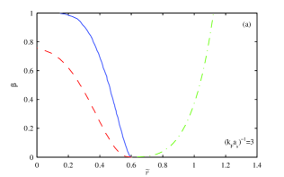
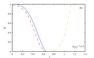
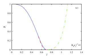
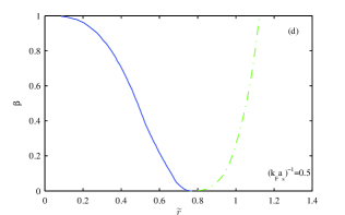
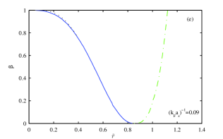
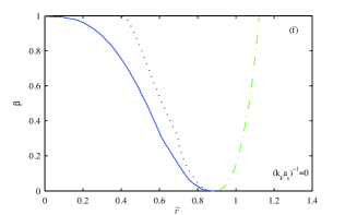
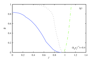
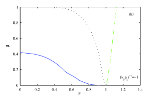
Figure 1: (Color Online) The zero temperature phase boundaries of a polarized Fermi gas in a trap with (a)$(k_{F}a_{s})^{-1}=3$, (b) $(k_{F}a_{s})^{-1}=1.5$, (c) $(k_{F}a_{s})^{-1}=1$, (d) $(k_{F}a_{s})^{-1}=0.5$, (e) $(k_{F}a_{s})^{-1}=0.09$, (f) $(k_{F}a_{s})^{-1}=0$, (g) $(k_{F}a_{s})^{-1}=-0.4$, (h) $(k_{F}a_{s})^{-1}=-1$. The solid lines mark the phase boundaries between the superfluid region (SF/BP1) and the normal region (NM/NP); the dashed lines are the phase boundaries between the SF phase and the BP1 phase; the dotted lines show the range of the minority spin component in the normal phase, which are effectively the phase boundaries between the NM and the NP phase; and the dash-dotted lines mark the range of the majority spin component in the normal phase. The trap radius $\widetilde{r}$ is in the units of the Thomas-Fermi radius for the corresponding directions.

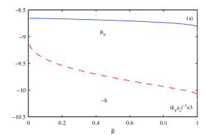
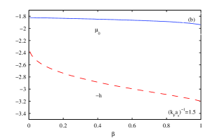
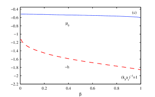
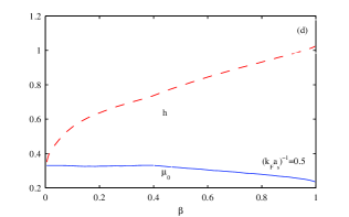
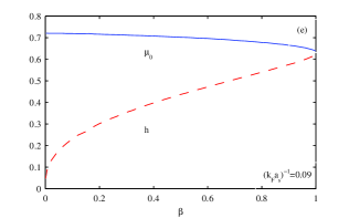
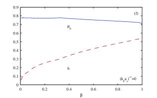
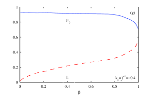
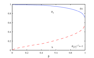
Figure 2: (Color Online) The chemical potential $\mu_{0}$ and the chemical potential difference $h$ as functions of population imbalance at zero temperature for: (a)$(k_{F}a_{s})^{-1}=3$, (b) $(k_{F}a_{s})^{-1}=1.5$, (c) $(k_{F}a_{s})^{-1}=1$, (d) $(k_{F}a_{s})^{-1}=0.5$, (e) $(k_{F}a_{s})^{-1}=0.09$, (f) $(k_{F}a_{s})^{-1}=0$, (g) $(k_{F}a_{s})^{-1}=-0.4$, (h) $(k_{F}a_{s})^{-1}=-1$. The solid lines represent $\mu_{0}/E_{F}$, the average chemical potential at the center of the trap; and the dashed lines are $h/E_{F}$ ($-h/E_{F}$ in (a-c) for better comparison with $\mu_{0}/E_{F}$), where the unit of energy $E_{F}$ is defined in Sec. II.

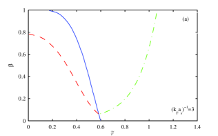
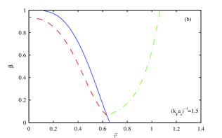
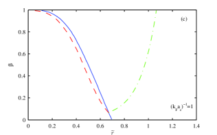
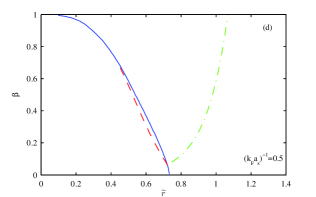
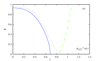
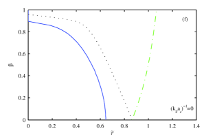
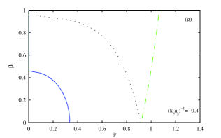
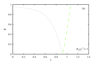
Figure 3: (Color Online) The finite temperature phase boundaries of a polarized fermion gas in a trap with (a)$(k_{F}a_{s})^{-1}=3$, (b) $(k_{F}a_{s})^{-1}=1.5$, (c) $(k_{F}a_{s})^{-1}=1$, (d) $(k_{F}a_{s})^{-1}=0.5$, (e) $(k_{F}a_{s})^{-1}=0.1$, (f) $(k_{F}a_{s})^{-1}=0$, (g) $(k_{F}a_{s})^{-1}=-0.4$, (h) $(k-Fa_{s})^{-1}=-1$. The solid lines mark the phase boundaries between the gapped and the gapless region; the dashed lines are the phase boundaries between the gapped phases without a Fermi surface and the ones that have; the dotted lines show the zero point of chemical potential of the minority spin component in the normal phase; and the dash-dotted lines show the zero point of the chemical potential of the majority spin component in the normal phase. The temperature is taken to be $T=0.22T_{F}$, which corresponds to a real temperature $T\sim 300nK$ for $2.7\times 10^{7}$ fermionic ${}^{6}Li$ atoms in a cigar shaped trap with $\omega_{z}\sim 23Hz,\omega_{x}=\omega_{y}\sim 110Hz$ 2 .

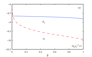
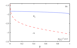
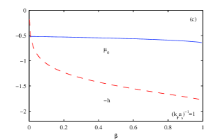
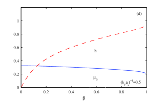
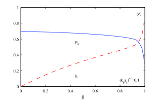
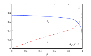
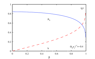
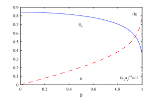
Figure 4: (Color Online) Same as Fig. 2, but $\mu$ and $h$ are shown as functions of population imbalance at finite temperature ($T=0.22T_{F}$) with: (a)$(k_{F}a_{s})^{-1}=3$, (b) $(k_{F}a_{s})^{-1}=1.5$, (c) $(k_{F}a_{s})^{-1}=1$, (d) $(k_{F}a_{s})^{-1}=0.5$, (e) $(k_{F}a_{s})^{-1}=0.1$, (f) $(k_{F}a_{s})^{-1}=0$, (g) $(k_{F}a_{s})^{-1}=-0.4$, (h) $(k-Fa_{s})^{-1}=-1$. The solid lines represent $\mu/E_{F}$; and the dashed lines are $h/E_{F}$

Figure 1 shows the detailed phase distribution in the trap at different interaction strengths $(k_{F}a_{s})^{-1}$ (corresponding to different magnetic field detunings). On the BEC side of the resonance (Fig.1(a), with $(k_{F}a_{s})^{-1}=3$) and at small but nonzero population imbalances, the Fermi gas separates into three phases in the trap: an SF core at the center, a BP1 phase in the middle, and an NP phase at the edge of the trap with only the majority spin component. As the imbalance parameter $\beta$ increases, the superfluid core becomes smaller until it vanishes at a critical imbalance, beyond which only the BP1 phase and the normal phase exist in the trap. This critical imbalance where the phase transition from the SF phase to the BP1 phase occurs becomes greater towards the resonance, while the parameter range of the BP1 phase shrinks (Fig. 1(b)(c)). At $(k_{F}a_{s})^{-1}=1$, the BP1 phase only exists at small population imbalances in a slim region bordering the SF and the NP phase (Fig. 1(c)). Within our numerical resolution ($\delta\beta\sim\pm 1\%$), the BP1 phase disappears at roughly $(k_{F}a_{s})^{-1}\sim 0.5$, on the BEC side of the resonance. Note that from numerical analysis, we find that the unpaired fermions in this BP1 phase are within the momentum range $0<\left|\mathbf{k}\right|<k_{+}$ (which implies $|\mu_{\mathbf{r}}|<\sqrt{h^{2}-|\Delta|^{2}}$ in this region), where $k_{+}$ is given in the previous section. In this BP1 phase, we therefore have the following phase separation picture in the momentum space: the paired fermions in the superfluid fill the outside momentum shell, while the unpaired fermions of the majority spin component occupy the states inside the Fermi ball with $\left|\mathbf{k}\right|<k_{+}$.

Once the BP1 phase disappears, the trap is left with only the SF phase and the NP phase over a certain range of the interaction strength (Fig. 1(d), with $(k_{F}a_{s})^{-1}\sim 0.5$). This continues till a new normal state, the NM phase shows up at large population imbalances at roughly $(k_{F}a_{s})^{-1}\sim 0.1$ (Fig. 1(e)), where fermions of both spin components show up in the normal gas, with different Fermi surfaces for different spins. The range of the NM phase grows towards the resonance, and at resonance or on the BCS side (Fig. 1(f)(g)(h)), the Fermi gas typically phase separates into three regions at small $\beta$: the SF phase, the NM phase and the NP phase. The superfluid phase disappears at a critical population imbalance, where the gas undergoes a phase transition from the superfluid phase to the normal state. Qualitatively, this picture agrees pretty well with the recent experimental findings 2 , although quantitatively, the mean-field type approximation at $T=0$ may somewhat overestimate the critical population imbalance for the disappearance of the SF core at the trap center.

To give more detailed information of this system, we also show in Fig. 2 the chemical potential $\mu_{0}$ at the trap center and the chemical potential difference $h$ as functions of the population imbalance $\beta$ at the corresponding interaction strengths $(k_{F}a_{s})^{-1}$. Note that the chemical potential difference $h$ between the two spin components does not change across the trap. The local chemical potential $\mu_{\mathbf{r}}$ changes, but given $\mu_{0}$ and the trap potential $V(\mathbf{r)}$, it changes through the simple relation $\mu_{\mathbf{r}}=\mu_{0}-V(\mathbf{r)}$ under the local density approximation. With the information given in Fig. 2, we know the local chemical potential $\mu_{\mathbf{r\sigma}}$ for each spin component $\mathbf{\sigma}$, and it becomes straightforward to calculate other properties of the system, such as the density profiles.

IV Phase Boundaries at Finite Temperature

At finite temperature, we calculate the total gap ($\Delta$) in the trap, from which we get the boundary between the gapped region and the gapless region. As the order parameter for the superfluid phase $\Delta_{s}$ is smaller than the total gap at finite temperature, the boundary between the gapped and the gapless regions serves as an upper bound for the superfluid phase note4 . At finite temperature, due to the thermal excitations, the atom density profiles change more smoothly as one goes from the trap center to the edge, so one cannot easily use the discontinuity of the density profiles to fix the boundary between the BP1 phase and the SF phase, nor the boundary between the different normal states (NM/NP). However, one can still look at the changes of the Fermi surfaces in the momentum space, which provides an unambiguous signal to determine the boundaries between different phase/regions. We should caution, however, that these boundaries do not necessarily correspond to sharp edges in the atom density profiles. For instance, in the normal phase with $\Delta=0$, when one of the chemical potentials, say $\mu_{\mathbf{r\uparrow}}$, changes its sign at the trap edge, which implies the disappearance of the Fermi surface for the spin up atoms as one moves outside (under the local density approximation), the density distribution of the spin up atoms does not vanish at that point. Instead, it will follow an exponential decay as the corresponding chemical potential turns negative. So, although these boundaries do not represent sharp spatial edges of the corresponding spin components, they indeed give a good estimation of the ranges.

The results of our calculation at finite temperature are shown in Fig. 3. We take the temperature $T=0.22T_{F}$, which corresponds to $T\sim 300nK$ with the experimental parameters in Ref. 2 (see caption of Fig. 3). The phase diagrams are qualitatively similar to those in Fig. 1, but there are several important differences at finite T which deserve to be emphasized. First of all, on the BEC side, the finite temperature BP1 region does not show up until a critical population imbalance (see Fig. 3(a-d)). The basic reason behind this feature is that at finite temperature, the population imbalance can be carried by the quasiparticle excitations in the conventional BCS superfluid state, as we have emphasized in 9c . Therefore, different from the zero temperature case, the conventional BCS state becomes partially polarized when there is a population imbalance, which significantly relaxes the competition between the population imbalance and the Cooper pairing, and which makes the momentum-space phase separation between the paired state and the excess fermions (the BP1 phase) unnecessary at small population imbalances. Secondly, the range of the BP1 region changes significantly from the zero temperature case. At $T=0.22T_{F}$, the BP1 region disappears near $(k_{F}a_{s})^{-1}\sim 0.15$, where there already exists an NM region in the phase diagram (see Fig. 3(d)(e)), which initially appears near $(k_{F}a_{s})^{-1}\sim 0.3$ for small population imbalance. Last but not least, at resonance or on the BCS side, the critical population imbalance at which the gapped region disappears at the center of the trap, which is an upper bound for the actual critical imbalance bordering the SF phase and the non-condensed pairs, becomes significantly smaller than the critical population imbalance at zero temperature (see Fig. 3(f)(g)(h)). The results above demonstrate that the phase boundaries, as well as the evolution of the different phases as the field sweeps across the crossover region, can be significantly affected by temperature. As all the experiments are necessarily done at a finite temperature, this suggests that it may be important to take the thermal effects into account for a quantitative interpretation of the experimental data.

At finite temperature, we also calculate the chemical potentials $\mu_{\mathbf{r\sigma}}$ as functions of the population imbalance $\beta$ at various interaction strengths $(k_{F}a_{s})^{-1}$, in order to provide detailed information of this system. The results are shown in Fig. 4. The properties can be directly read from the figure, and as the main features there are qualitatively similar to those in Fig. 2 for the zero temperature case, we neglect the detailed discussion here.

V Summary

In summary, we provide detailed calculations of the phase diagrams for a trapped Fermi gas with population imbalance over the entire BCS-BEC crossover region at zero and at finite temperature. The calculation is done with the self-consistent $G_{0}G$ diagram scheme. We also emphasize the importance of using the universal dimensionless equations. The properties of the system then only depend on three dimensionless parameters, from which we can calculate the universal phase diagrams valid for different atom species with different atom numbers under various trap configurations. The main results of our calculation are shown in Fig. 1 and 3, with their prominent features discussed in detail in the corresponding sections.

We thank Martin Zwierlein for helpful discussions. This work was supported by the NSF awards (0431476), the ARDA under ARO contracts, and the A. P. Sloan Fellowship.

References

- (1) C.A. Regal, M. Greiner and D.S. Jin, Phys. Rev. Lett. 92, 040403 (2004); M.W. Zwierlein et al., Phys. Rev. Lett. 92, 120403 (2004); C. Chin et al., Science 305, 1128 (2004).
- (2) M.W. Zwierlein, A. Schirotzek, C.H. Schunck, and W. Ketterle, Science 311, 492 (2006).
- (3) G.B. Partridge, W. Li, R.I. Kamar, Y. Liao, and R.G. Hulet, Science 311, 503 (2006).
- (4) G. Sarma, J. Phys. Chem. Solids 24, 1029 (1963).
- (5) P. Fulde and R. A. Ferrell, Phys. Rev. 135, A550 (1964); A.I. Larkin and Y.N. Ovchinnikov, Sov. Phys. JETP 20, 762 (1965).
- (6) R. Casalbuoni, G. Nardulli, Rev. Mod. Phys. 76, 263 (2004).
- (7) W.V. Liu and F. Wilczek, Phys. Rev. Lett. 90, 047002 (2003); M. M. Forbes et al., Phys.Rev.Lett. 94, 017001 (2005).
- (8) P. F. Bedaque, H. Caldas, and G. Rupak, Phys. Rev. Lett. 91, 247002 (2003); A. Sedrakian et al. Phys. Rev. A 72, 013613 (2005); J. Carlson and S. Reddy, Phys. Rev. Lett. 95, 060401 (2005).
- (9) C.-H. Pao, S.-T. Wu, and S.-K. Yip, cond-mat/0506437.
- (10) D.E. Sheehy and L. Radzihovsky, Phys. Rev. Lett. 96, 060401 (2006).
- (11) P. Pieri, G.C. Strinati, cond-mat/0512354.
- (12) J. Kinnunen, L.M. Jensen, P. Torma, Phys. Rev. Lett. 96, 110403 (2006).
- (13) W. Yi, L.-M. Duan, Phys. Rev. A 73, 031604(R) (2006).
- (14) F. Chevy, cond-mat/0601122.
- (15) T.N. De Silva, E.J. Mueller, cond-mat/0601314.
- (16) M. Haque, H.T.C. Stoof, condmat/0601321.
- (17) T.-L. Ho, H. Zhai, cond-mat/0602568.
- (18) K. Yang, cond-mat/0603190; Z.-C. Gu; G. Warner; F. Zhou, cond-mat/0603091; M. Iskin, C. A. R. Sa de Melo, cond-mat/0604184; K. Machida, T. Mizushima, M. Ichioka, cond-mat/0604339.
- (19) Q.J. Chen, et al., Phys. Rep. 412, 1 (2005); Phys. Rev. Lett. 95, 260406 (2005).
- (20) A.J. Leggett, in Modern Trends in the Theory of Condensed Matter (Springer-Verlag, Berlin, 1980), pp. 13-27.
- (21) R.B. Diener, T.-L. Ho, cond-mat/0405174 (2004); W. Yi, L.-M. Duan, cond-mat/0603264.
- (22) Although there is an indication that the FFLO state might exist near resonance in a narrow boundary region in the trap9b , we have not yet found evidence for the existence of such a state which is stable in the strongly interacting region through numerical search within the local density approximation.
- (23) T.-L. Ho, Phys. Rev. Lett. 92, 090402 (2004).
- (24) If the trap has anharmonicity which is a constant expressed in the unit of the Thomas-Fermi radius (see M. W. Zwierlein, W. Ketterle, cond-mat/0603489), we will still have the same universality as discussed in the text.
- (25) Note that this state is also called the polarized (magnetized) superfluid state in the literature 8a . However, at finite temperature, the normal BCS superfluid state also has finite polarization as emphasized in Ref. 9c . To distinguish between these different kinds of superfluid phases, we call the non-BCS superfluid as the BP1 phase (abbreviation for the breached pair phase with one Fermi surface), similar to the terminology of Ref. 7 . The breached pair state was studied in Ref. 7 on the BCS side, where it has two coexisting Fermi surfaces (BP2 phase). Other than that difference, the properties of the BP1 and BP2 phases are pretty much the same. For instance, they are both superfluid states with gapless fermionic excitations, and are both homogeneous in the real space while phase separated in the momentum space.
- (26) To exactly fix the phase boundary for the superfluid phase at finite , one needs to derive the dispersion relation for the pair excitations to split into and . This dispersion relation is known for the equal-population case 10 , but has not yet been derived for the case with population imbalance within the self-consistent scheme. However, for the calculation of the total gap and the atom density profiles, one does not need to fix that dispersion relation 9c .