Electron interactions in graphene in a strong magnetic field

Abstract

Graphene in the quantum Hall regime exhibits a multi-component structure due to the electronic spin and chirality degrees of freedom. While the applied field breaks the spin symmetry explicitly, we show that the fate of the chirality SU(2) symmetry is more involved: the leading symmetry-breaking terms differ in origin when the Hamiltonian is projected onto the central ($n=0$) rather than any other Landau levels. Our description at the lattice level leads to a Harper equation; in its continuum limit, the ratio of lattice constant $a$ and magnetic length $l_{B}$ assumes the role of a small control parameter in different guises. The leading symmetry-breaking terms are lattice effects, algebraically small in $a/l_{B}$. We analyze the Haldane pseudopotentials for graphene, and evaluate the easy-plane anisotropy of the graphene ferromagnet.

Introduction: The recent discovery novoselov1 ; zhang1 of an integer quantum Hall (QH) effect in a two-dimensional (2D) sheet of graphite, known as graphene, has triggered an avalanche of activity, including on the theory side studies of the transport properties of relativistic Dirac particles,gusynin ; katsnelson ; peres the analysis of edge states CN ; brey ; abanin and shot noise bjoern as well as Berry phases in bilayers.mccann

In a simple model, electrons in graphene can be treated as hopping on a honeycomb lattice.wallace ; slon Perhaps the most salient feature of this problem is the existence in the band structure of a pair of Dirac points with a linear (‘relativistic’) energy-momentum relationship. These points are located at the two inequivalent corners of the Brillouin zone (labelled by $K$ and $K^{\prime}=-K$), endowing graphene with a multi-component structure analogous to the well-studied examples of bilayer systems, the multi-valley structure of Silicon and of course the simple spin degree of freedom. These degrees of freedom can be thought of as SU(2) (or higher symmetry) pseudospins. The resulting Hamiltonian typically contains symmetric terms as well as ones which lower the symmetry, such as Zeeman (spin) or capacitance (bilayer) moon energies.

Here, we argue that graphene may be viewed as a further type of multi-component system. Its internal degree of freedom can be thought of as a chirality:haldane the wavevectors $K$ and $K^{\prime}$ encode the (anti)clockwise variation of the phase of the electronic wavefunction on the three sites neighboring any given site on one sublattice.

Moreover, we show that for $n\neq 0$ the chiral SU(2) symmetry is reduced to U(1) in graphene, due to backscattering terms with momentum transfer $2K\sim K$ which provide a coupling of the chirality to the orbital part of the wavefunction. On the contrary, in $n=0$, the broken symmetry may be due to electrostatic (“Hartree”) effects. Although different in origin, both effects are of order $O(a/l_{B})$. The distance between neighboring carbon atoms $a\simeq 0.14{\rm nm}$ provides an additional lengthscale besides the magnetic length $l_{B}=\sqrt{\hbar/eB}=26{\rm nm}/\sqrt{B[{\rm T}]}$, so that $a\ll l_{B}$. It is somewhat analogous to the layer separation $d$ for bilayers. In graphene for $n\neq 0$, however, only the exchange part of the symmetry-breaking interaction is non-zero, whereas in bilayers the direct term encodes the capacitance energy, which can be important already for typical values of $d/l_{B}\sim 1$.

In the following, we flesh out this picture with a microscopic calculation starting at the lattice level, in which we derive and discuss the effective model for interacting electrons restricted to a single relativistic LL and compare it to the non-relativistic case of electrons in conventional semiconductor heterostructures; the difference between the two is most significant for $n=1$. The backscattering terms are discussed in the case of the QH ferromagnet at the filling factors $\bar{\nu}=1$ of the partially filled LL (for an arbitrary LL, we have $\nu=4n+\bar{\nu}$).

The model: The electron field in graphene may be written as a two-spinor whose components, $\psi_{\sigma}({\bf r})=\exp(i\sigma{\bf K}\cdot{\bf r})\chi_{\sigma}({\bf r})$, are a product of a slowly varying part $\chi_{\sigma}({\bf r})$ and a rapidly oscillating plane wave with $\sigma{\bf K}=\sigma(4\pi/3\sqrt{3}a){\bf e}_{x}$ for the Brillouin zone corners $K$ and $K^{\prime}$ (chiralities $\sigma=\pm 1$, respectively). The components of each two-spinor field $\chi_{\sigma}({\bf r})$ correspond to the two triangular sublattices (labelled by $\alpha=\pm 1$) of the bipartite honeycomb lattice. In a magnetic field with the Landau gauge ${\bf A}=(0,Bx)$, $q_{y}$ is a good quantum number, and we may expand $\chi_{\alpha}({\bf r})=\exp(iq_{y}y)g_{\alpha}(y)$. The electron dynamics (in a tight-binding model with nearest-neighbor hopping $t=1$) is governed by the Harper equation

$$Eg_{\alpha}^{\sigma}(x) = -2\cos\left\{\sigma\frac{2\pi}{3}+\frac{\sqrt{3}}{2}\left[q_{y}+\frac{\left(x+\alpha/4\right)}{l_{B}^{2}}\right]\right\}$$ (1)

$$\times g_{-\alpha}^{\sigma}\left(x+\frac{\alpha}{2}\right)-g_{-\alpha}^{\sigma}(x-\alpha),$$

where the distances are measured in units of $a$. In order to derive a continuum limit in the presence of an unbounded vector potential ${\bf A}$, one expands the cosine in Eq. (1) in the vicinity of $x_{\mu}$ defined as $[q_{y}+\alpha x_{\mu}(q_{y})/l_{B}^{2}]\sqrt{3}/2=2\pi\mu$, where $\mu$ is an integer which effectively acts as an additional quantum number besides the quasimomentum $q_{y}$ in the first Brillouin zone.

The continuum limit of Eq. (1) thus reads

$$Eg_{\alpha}^{\sigma}(x)=\frac{3}{2}\left(\alpha l_{B}\partial_{x}+\sigma\frac{x}{l_{B}}\right)g_{-\alpha}^{\sigma}(x),$$

where $x$ is now a small deviation from $x_{\mu}$. This result coincides with the ones obtained by introducing the minimal coupling ${\bf p}\rightarrow{\bf p}+e{\bf A}$ after deriving the $B=0$ continuum theory. haldane ; LLquant Note that the typical extension of the wavefunctions along the $x$-axis is $R_{L}\propto\sqrt{n}l_{B}$ in the $n$-th LL, and the periodicity of $x_{\mu}$ is $\sim l_{B}^{2}/a$. The overlap between wavefunctions with differing $\mu$ is therefore exponentially suppressed provided $\sqrt{n}\ll l_{B}/a$. Finally,

$$\chi_{+}({\bf r})=\frac{1}{\sqrt{2}}\sum_{n,m}\left(\begin{array}[]{c}i\sqrt{1+\delta_{n,0}}\langle{\bf r}|\,|n|,m\rangle\\ {\rm sgn}(n)\langle{\bf r}|\,|n|-1,m\rangle\end{array}\right)c_{n,m;+}\ ,$$ (4)

where the index $+$ represents the $K$ point. In the expression for $\chi_{-}$ (at $K^{\prime}$), the components of the spinor are reversed. Here ${\rm sgn}(n)=\{1,0,-1\}$ for $n\{>,=,<\}0$, respectively. The quantum number $n$ is the index of the relativistic LL, and $m$ is associated to the guiding center operator, which commutes with the one-particle Hamiltonian. The $|n,m\rangle$ are the usual (non-relativistic) one-particle states for a charged particle in a perpendicular magnetic field. The $c_{n,m;\sigma}$ are fermionic destruction operators.

Projection onto a LL ($n\neq 0$) of the sublattice densities $\rho_{\alpha}({\bf r})=\sum_{\sigma,\sigma^{\prime}}\psi_{\sigma,\alpha}^{\dagger}({\bf r})\psi_{\sigma^{\prime},\alpha}({\bf r})$ gives

$$\rho^{n}({\bf q})=\rho_{1}^{n}({\bf q})+\rho_{2}^{n}({\bf q})=\sum_{\sigma,\sigma^{\prime}}F_{n}^{\sigma\sigma^{\prime}}({\bf q})\bar{\rho}^{\sigma\sigma^{\prime}}({\bf q}),$$ (5)

where the projected density operators read $\bar{\rho}^{\sigma\sigma^{\prime}}({\bf q})=\sum_{m,m^{\prime}}\langle m|\exp\{-i[{\bf q}+(\sigma-\sigma^{\prime}){\bf K}]\cdot{\bf R}\}|m^{\prime}\rangle c_{n,m,\sigma}^{\dagger}c_{n,m^{\prime},\sigma^{\prime}}$. The operator ${\bf R}$ represents the usual guiding center position, and $\eta$ is the cyclotron coordinate, ${\bf r}={\bf R}+\mbox{\boldmath$\eta$}$. The chirality-dependent form factors $F_{n}^{\sigma\sigma^{\prime}}({\bf q})$ read, in terms of associated Laguerre polynomials $L_{n}^{\alpha}(x)$:

$$F_{n}^{++}({\bf q}) = \frac{1}{2}\left[L_{|n|}\left(\frac{|{\bf q}|^{2}}{2}\right)+L_{|n|-1}\left(\frac{|{\bf q}|^{2}}{2}\right)\right]e^{-|{\bf q}|^{2}/4},$$

$$F_{n}^{+-}({\bf q}) = \left(\frac{-(q+q^{*}-K-K^{*})}{2\sqrt{2|n|}}\right)$$

$$\times L_{|n|-1}^{1}\left(\frac{|{\bf q}-{\bf K}|^{2}}{2}\right)e^{-|{\bf q}-{\bf K}|^{2}/4},$$

where $q=q_{x}+iq_{y}$ and $K=K_{x}+iK_{y}$ are written in complex notation, and the wave vectors are given in units of $1/l_{B}$. $F_{n}^{++}({\bf q})=F_{n}^{--}({\bf q})$, and $F_{n}^{-+}({\bf q})$ is obtained by replacing ${\bf q}\to-{\bf q}$ in $F_{n}^{+-}({\bf q})$.

The Hamiltonian of interacting electrons in graphene, projected onto a single relativistic LL thus reads

$$H=\frac{1}{2}\sum_{\sigma_{1},...,\sigma_{4}}\sum_{{\bf q}}v_{n}^{\sigma_{1},...,\sigma_{4}}({\bf q})\bar{\rho}^{\sigma_{1}\sigma_{3}}(-{\bf q})\bar{\rho}^{\sigma_{2}\sigma_{4}}({\bf q}),$$ (6)

where the sum over the wave vectors is restricted to the first Brillouin zone. Indeed, the potential consists of a sum over reciprocal lattice vectors, as the local densities [Eq. (5)], valid for $l_{B}\gg a$, are restricted to the hexagonal lattice. The chirality-dependent effective interaction

$$v_{n}^{\sigma_{1},...,\sigma_{4}}({\bf q})=\frac{2\pi e^{2}}{\epsilon|{\bf q}|}F_{n}^{\sigma_{1}\sigma_{3}}(-{\bf q})F_{n}^{\sigma_{2}\sigma_{4}}({\bf q})$$ (7)

is not SU(2) symmetric; however, the symmetry-breaking terms are suppressed parametrically in $a/l_{B}$. To see this, consider the different form-factor combinations in the effective interaction potential (Electron interactions in graphene in a strong magnetic field).
– Terms of the form $F_{n}^{\sigma,\sigma}(\mp{\bf q})F_{n}^{\sigma^{\prime},-\sigma^{\prime}}(\pm{\bf q})$ and “umklapp scattering” terms [$F_{n}^{\sigma,-\sigma}(-{\bf q})F_{n}^{\sigma,-\sigma}({\bf q})$] are exponentially small in $a/l_{B}$.
– “Backscattering” [$F_{n}^{\sigma,-\sigma}(-{\bf q})F_{n}^{-\sigma,\sigma}({\bf q})$]: one obtains $v_{n}^{+--+}({\bf q})\sim\exp(-|{\bf q}|^{2}/2)/|{\bf q}^{\prime}\pm{\bf K}|\sim\exp(-|{\bf q}|^{2}/2)/|{\bf K}|,$ which is only algebraically small, $v_{n}^{+--+}/(e^{2}/\epsilon l_{B})\sim a/l_{B}$, and thus constitutes the leading perturbation to the remaining [SU(2) invariant] terms.

These leading-order terms in the effective interaction yield the SU(2) [or SU(4), if the physical spin is also taken into account] symmetric Hamiltonian (for $n\neq 0$)

$$H_{eff}^{n}=\frac{1}{2}\sum_{\sigma,\sigma^{\prime}}\sum_{{\bf q}}\frac{2\pi e^{2}}{\epsilon|{\bf q}|}\left[\mathcal{F}_{n}(q)\right]^{2}\bar{\rho}_{\sigma}(-{\bf q})\bar{\rho}_{\sigma^{\prime}}({\bf q}),$$ (8)

with the graphene form factor

$$\mathcal{F}_{n}(q)=\frac{1}{2}\left[L_{|n|}\left(\frac{q^{2}}{2}\right)+L_{|n|-1}\left(\frac{q^{2}}{2}\right)\right]e^{-q^{2}/4}$$ (9)

and $\bar{\rho}_{\sigma}({\bf q})\equiv\bar{\rho}^{\sigma\sigma}({\bf q})$. The graphene form factor (9) has already been written down by Nomura and MacDonald in their study of the QH ferromagnetism at $\bar{\nu}=1$.macdonald The leading-order symmetry-breaking correction due to backscattering is (with $v_{n}^{\sigma,-\sigma}({\bf q})\equiv v_{n}^{\sigma,-\sigma,-\sigma,\sigma}({\bf q})$)

$$H_{bs}=\frac{1}{2}\sum_{\sigma}\sum_{{\bf q}}v_{n}^{\sigma,-\sigma}({\bf q})\bar{\rho}^{\sigma,-\sigma}(-{\bf q})\bar{\rho}^{-\sigma,\sigma}({\bf q}).$$ (10)

The central level ($n=0$) behaves remarkably differently. In this case, the electron chirality $\sigma$ is equivalent to the sublattice index $\alpha$ (Eq. 4), and therefore

$$\rho_{\alpha}^{n=0}({\bf q})=e^{-q^{2}/4}\sum_{m,m^{\prime}}\langle m|e^{-i{\bf q}\cdot{\bf R}}|m^{\prime}\rangle c_{n,m;\alpha}^{\dagger}c_{n,m^{\prime};\alpha}$$

with the same form factor $\mathcal{F}_{n=0}(q)=e^{-q^{2}/4}$ as for non-relativistic electrons in the lowest LL. From an electrostatic point of view, it may be energetically favorable to distribute the electronic density with equal weight on both sublattices. For $n\neq 0$, this follows directly from Eq. (4), but in $n=0$, an equal-weight superposition of $\sigma=\pm 1$ is required to distribute the charges homogeneously on both sublattices. Such an electrostatic effect, compared to the SU(2) invariant terms, is of the same order $O(a/l_{B})$ as the backscattering term in $n\neq 0$.

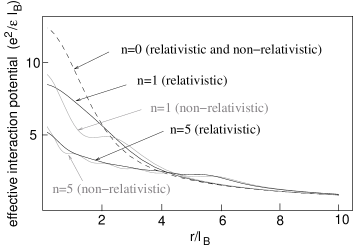
Figure 1: Effective interaction potentials in real space: comparison between the relativistic (black lines) and non-relativistic (gray lines) LLs $n=0,1$, and $5$. The dashed line represents the interaction potential in $n=0$, which is the same for relativistic and non-relativistic electrons.

Effective interaction: By absorbing the form factor into the interaction, we define

$$v_{n}(q)=\frac{2\pi e^{2}}{\epsilon q}\left[\mathcal{F}_{n}(q)\right]^{2}.$$ (11)

Fig. 1 shows the effective interaction potentials (11) transformed to real space, for $n=0,1$, and $5$. At large distances, the usual $1/r$ Coulomb potential is obtained. Interestingly, the shape of the interaction potential for the relativistic $n=1$ LL in graphene is more similar to the non-relativistic $n=0$ level than to the corresponding one $n=1$, as may also be seen in a pseudopotential expansion,haldane2 $V_{\ell}^{n}=(2\pi)^{-1}\sum_{{\bf q}}v_{n}(q)L_{\ell}(q^{2})\exp(-q^{2}/2).$ Indeed the ratios $V_{2m+1}/V_{2m+3}$ for the odd integer pseudopotentials, which are relevant for the case of polarized electrons, decrease monotonically both in $n=1$ and $n=0$ for relativistic LLs. These ratios, and the differences $V_{2m-1}-V_{2m+1}$ are bigger in the former case, so that – among the polarized states – fractional QH states will therefore be more stable in $n=1$ than in $n=0$ (at constant magnetic field). By contrast, candidate chirality unpolarized states (such as at $\nu=2/3$) fare better, for two reasons: firstly, the fact that the relativistic effective potential is more short-ranged in $n=0$ than in $n=1$ leads to $V_{0}$ (and $V_{0}/V_{1}$) being smaller for $n=1$. Secondly, the pair of internal SU(2) degrees of freedom allow for a smaller unpolarized ’composite Fermi sphere’.

Numerical results RH show a first-order phase transition at $V_{1}/V_{3}\simeq 1.3$ between the Pfaffian state MR at $\bar{\nu}=1/2$ and a charge-density wave,CDW and a crossover to a composite-fermion Fermi sea when $V_{1}/V_{3}$ is further increased. The Pfaffian state is absent in $n=0$, where $V_{1}^{0}/V_{3}^{0}=1.6$, probably due to an inaccessibly small gap. RH In the relativistic $n=1$ LL, one finds an even larger ratio $V_{1}^{1}/V_{3}^{1}=1.67$ so that a Pfaffian state is also unlikely to be observed there. Even though the ratio $V_{1}^{2}/V_{3}^{2}=1.16$ in the relativistic $n=2$ LL is larger than in the corresponding non-relativistic level ($V_{1}^{2}/V_{3}^{2}=1.14$), it is well below the critical ratio, and one would thus expect a stripe phase at $\bar{\nu}=1/2$.

It is straightforward to check that the difference to the non-relativistic case vanishes, in the large-$n$ limit (see Fig. 1 for $n=5$), i.e. far from the Dirac points. Replacing $L_{n}(q^{2}/2)\exp(-q^{2}/4)\simeq J_{0}(q\sqrt{2n+1}),$ the envelope of $\mathcal{F}^{2}_{n}(q)\simeq\left[J_{0}(q\sqrt{2n-1})+J_{0}(q\sqrt{2n+1})\right]^{2}/4\simeq J^{2}_{0}(q\sqrt{2n})$ agrees to leading order in $n$ with the non-relativistic case.

QH ferromagnet at $\bar{\nu}=1$: In recent transport measurements on a single graphene sheet additional integer QH plateaux beyond those corresponding to $\nu=4n$ have been observed.zhang2 These appear as the first signature of electron-electron interactions, and the analogy with the non-relativistic case in semiconductor heterostructures hints at a chirality QH ferromagnet. The stability of such a state, in the presence of impurities, has been investigated by Nomura and MacDonald.macdonald We now analyze the impact of the backscattering term (10) on such a ferromagnet for $n\neq 0$, within the Hartree-Fock (HF) approximation. Following Ref. moon, , we consider the HF trial state $|\Psi\rangle=\prod_{m}(u_{m}c_{m,+}^{\dagger}+v_{m}c_{m,-}^{\dagger})|0\rangle,$ where we may parametrize $u_{m}=\cos(\theta_{m}/2)e^{-i\phi_{m}/2}$ and $v_{m}=\sin(\theta_{m}/2)e^{i\phi_{m}/2}$, in terms of the real angle fields $\theta_{m}$ and $\phi_{m}$, which can be thought of as polar coordinates of a vector field ${\bf n}(m)$. In the case of a SU(2)-symmetric repulsive interaction, it has been shown that the trial state $|\Psi\rangle$ minimizes the energy for constant $\theta_{m}$ and $\phi_{m}$, thus yielding a simple ferromagnet.moon The backscattering term, averaged over this state, is, apart from an unimportant constant $C$,

$$\langle H_{bs}\rangle = \frac{1}{4}\sum_{m,m^{\prime}}\left\{V^{bs}_{m,m^{\prime},m,m^{\prime}}\left[n_{x}(m)n_{x}(m^{\prime})+x\rightarrow y\right]\right.$$ (12)

$$\left.+V^{bs}_{m,m^{\prime},m^{\prime},m}n_{z}(m)n_{z}(m^{\prime})\right\}+C,$$

$$V_{m_{1},...,m_{4}}^{bs} \simeq \frac{\pi e^{2}}{\epsilon|{\bf K}|}\sum_{{\bf q}}\frac{|{\bf q}|^{2}}{2|n|}\left[L_{|n|-1}^{1}\left(\frac{|{\bf q}|^{2}}{2}\right)e^{-|{\bf q}|^{2}/4}\right]^{2}$$ (13)

$$\times\langle m_{1}|e^{i{\bf q}\cdot{\bf R}}|m_{3}\rangle\langle m_{2}|e^{-i{\bf q}\cdot{\bf R}}|m_{4}\rangle.$$

The factor of $|q|^{2}$ in this sum is due to the fact that the wavefunctions on the same sublattice, but for different chiralities, are orthogonal. A gradient expansion moon yields to lowest order an easy-plane anisotropy $\Delta_{z}$:

$$\langle H_{bs}\rangle^{(0)}=\sum_{m}\Delta_{z}[n_{z}(m)]^{2},~{}~{}~{}\Delta_{z}=\frac{1}{16\pi^{2}}\frac{e^{2}}{\epsilon|{\bf K}|}.$$ (14)

This is reminiscent of the bilayer case, where a finite layer separation also induces easy-plane ferromagnetism. The key differences are: (i) the parameter $a/l_{B}\sim 10^{-2}$, which mimicks the “layer separation”, is tiny for currently experimentally accessible magnetic fields. This implies a Curie temperature $\Theta\sim e^{2}/k_{B}\epsilon l_{B}$, whereas the crossover to easy-plane behavior does not become visible until a logarithmically (in $a/l_{B}$) small energy. As chirality ferromagnetism involves neither electric nor magnetic dipole ordering, inter-plane coupling in a multi-layer system will be suppressed. This opens the perspective of probing the 2D behavior for instance in specific-heat measurements. (ii) Contrary to the bilayer case and the relativistic $n=0$ LL, the gap is not due to a charging energy when only one layer is filled – there is no contribution to Eq. (14) from the direct interaction because $v^{\pm}_{n}(q=0)=0$ [Eq. (7)]. (iii) $\Delta_{z}$ is a lattice effect – it vanishes linearly in $a$ as the lattice constant tends to zero at fixed $l_{B}$. It does not depend on $n$, whereas the SU(2) symmetric terms scale as $e^{2}/\epsilon\sqrt{n}$ in the large-$n$ limit. Note, however, that the continuum limit based on the Dirac equation ceases to be valid when $R_{L}\sim\sqrt{n}l_{B}\sim l_{B}^{2}/a$.

Comparison with experiment: Zhang et al. have observed additional Hall plateaux corresponding to $\nu=0,\pm 1\ (n=0)$ and $\nu=\pm 4\ (n=1)$.zhang2 The former pair corresponds to a complete resolution of the fourfold degeneracy of LLs corresponding to different internal (spin and chirality) degrees of freedom in $n=0$. An explanation of this has to consider the size of the disorder broadening of the LLs, $\Gamma$, compared to their splitting due to the cost of exciting quasiparticles away from integer filling.macdonald An experimental estimate yields $\Gamma\sim 1.7$meV. zhang2

Using our above results, we find that these quasiparticles are Skyrmions for $n=0,1$, whose energy cost $E_{sk}=4\pi\rho_{s}$ is obtained within the non-linear sigma model,moon with the help of the stiffness

$$\rho_{s}=\frac{1}{32\pi^{2}}\int_{0}^{\infty}dqq^{3}v_{n}(q).$$

One obtains for the experimentally relevant parameters (at $17$T with dielectric constantdiel $\epsilon\sim 5$) $E_{sk}=4\pi\rho_{s}=\frac{7}{64}\sqrt{\pi/2}e^{2}/\epsilon l_{B}\sim 1.8$meV ($n=1$) and, for $n=0$, $E_{sk}=\frac{1}{4}\sqrt{\pi/2}e^{2}/\epsilon l_{B}\sim 4$meV, both for SU(2) or SU(4).arovas In addition, there is a contribution from anisotropies, mainly the Zeeman effect (about $E_{Z}=0.1B$[T]meV); the chirality-symmetry breaking due to lattice effects, being of order $\sim 0.05$meV, play only a minor role here.

The activation gap at $\nu=\pm 4$ scales linearly with $B$, indicating a relevant Zeeman effect, and the plateau is visible from $\sim 17$T onwards. zhang2 Given the Skyrmions in $n=0$ are more costly than the sum of $E_{sk}$ and $E_{Z}$ in $n=1$, this explains why the chirality Landau levels are resolved at 17T in $n=0$, even without the help of an anisotropy field, whereas they remain absent at $\nu=\pm 3,\pm 5$ in fields up to 45T. In fact, for $n=1$, $E_{sk}$ does not reach 4meV for fields below 80T; also, the plateau at $\nu=0$ disappears below $11$T, where $E_{sk}\sim 3$meV.

To summarize, we have analyzed a microscopic model for interaction effects in graphene in the QH regime. We find corrections to the SU(2) chirality-symmetric model to be numerically much smaller than the Zeeman energy breaking the SU(2) spin-symmetry. In addition, the effective interaction potential differs from the non-relativistic case most strongly for small but nonzero $n$, in particular $n=1$, which will therefore a good place to look for interaction physics different from the GaAs heterostructure. Finally, recent experiments suggest the presence of chirality ferromagnetism and Skyrmions in graphene.

Note added: After submission of this manuscript, articles of related work appeared, by Alicea and Fisher AF on ferromagnetism at the integer QHE, and by Apalkov and Chakraborty AC on exact diagonalisations in the fractional QH regime using the above-mentioned pseudopotentials.

Acknowledgements: We thank N. Cooper, J.-N. Fuchs, D. Huse, P. Lederer, and S. Sondhi for fruitful discussions. M.O.G. is greatful for a stimulating interaction in the LPS’ “Journal Club Mesoscopic Physics”.

References

- (1) K. S. Novoselov, A. K. Geim, S. V. Morosov, D. Jiang, M. I. Katsnelson, I. V. Grigorieva, S. V. Dubonos, and A. A. Firsov, Nature 438, 197 (2005).
- (2) Y. Zhang, Y.-W. Tan, H. L. Stormer, and P. Kim, Nature 438, 201 (2005).
- (3) V. P. Gusynin and S. G. Sharapov, Phys. Rev. Lett. 95, 146801 (2005); Phys. Rev. B 73, 245411 (2006).
- (4) M. I. Katsnelson, Eur. Phys. J. B 51, 157 (2006)
- (5) N. M. R. Peres, F. Guinea, and A. H. Castro Neto, Phys. Rev. B 73, 125411 (2006).
- (6) A. Castro Neto, F. Guinea, and N. M. R. Peres, Phys. Rev. B 73, 205408 (2006).
- (7) L. Brey and H. A. Fertig, Phys. Rev. B 73, 195408 (2006).
- (8) D. A. Abanin, P. A. Lee, and L. S. Levitov, Phys. Rev. Lett. 96, 176803 (2006).
- (9) J. Tworzydlo, B. Trauzettel, M. Titov, A. Rycerz, and C. W. J. Beenakker, Phys. Rev. Lett. 96, 246802 (2006).
- (10) E. McCann and V. I. Fal’ko, Phys. Rev. Lett. 96, 086805 (2006).
- (11) P. R. Wallace, Phys. Rev. 71, 622 (1947).
- (12) J. C. Slonczewski and P. R. Weiss, Phys. Rev. 109, 272 (1958).
- (13) K. Moon, H. Mori, K. Yang, S. M. Girvin, A. H. MacDonald, I. Zheng, D. Yoshioka et S.-C. Zhang, Phys. Rev. B 51, 5138 (1995).
- (14) F. D. M. Haldane, Phys. Rev. Lett. 61, 2015 (1988).
- (15) Y. Zheng and T. Ando, Phys. Rev. B 65, 245420 (2002).
- (16) K. Nomura and A. H. MacDonald, Phys. Rev. Lett. 96, 256602 (2006).
- (17) F. D. M. Haldane, Phys. Rev. Lett. 51, 605 (1983).
- (18) G. Moore and N. Read, Nucl. Phys. B 360, 362 (1991).
- (19) E. H. Rezayi and F. D. M. Haldane, Phys. Rev. Lett. 84, 4685 (2000).
- (20) A. A. Koulakov, M. M. Fogler et B. I. Shklovskii, Phys. Rev. Lett. 76, 499 (1996); R. Moessner and J. T. Chalker, Phys. Rev. B 54, 5006 (1996).
- (21) Y. Zhang, Z. Jiang, J. P. Small, M. S. Purewal, Y.-W. Tan, M. Fazlollahi, J. D. Chudow, J. A. Jaszczak, H. L. Stormer, and P. Kim, Phys. Rev. Lett. 96, 136806 (2006).
- (22) J. González, F. Guinea, and M. A. H. Vozmediano, Phys. Rev. B 59, 2474 (1999).
- (23) D. P. Arovas, A. Karlhede, and D. Lilliehöök Phys. Rev. B 59, 13147 (1999).
- (24) J. Alicea and M. P. A. Fisher, Phys. Rev. B 74, 075422 (2006).
- (25) V. M. Apalkov and T. Chakraborty, Phys. Rev. Lett. 97, 126801 (2006).