Navier-Stokes transport coefficients of $d$-dimensional granular binary mixtures at low density

Abstract

The Navier-Stokes transport coefficients for binary mixtures of smooth inelastic hard disks or spheres under gravity are determined from the Boltzmann kinetic theory by application of the Chapman-Enskog method for states near the local homogeneous cooling state. It is shown that the Navier-Stokes transport coefficients are not affected by the presence of gravity. As in the elastic case, the transport coefficients of the mixture verify a set of coupled linear integral equations that are approximately solved by using the leading terms in a Sonine polynomial expansion. The results reported here extend previous calculations [V. Garzó and J. W. Dufty, Phys. Fluids 14:1476–1490 (2002)] to an arbitrary number of dimensions and provide explicit expressions for the seven Navier-Stokes transport coefficients in terms of the coefficients of restitution and the masses, composition, and sizes of the constituents of the mixture. In addition, to check the accuracy of our theory, the inelastic Boltzmann equation is also numerically solved by means of the direct simulation Monte Carlo method to evaluate the diffusion and shear viscosity coefficients for hard disks. The comparison shows a good agreement over a wide range of values of the coefficients of restitution and the parameters of the mixture (masses and sizes).

KEY WORDS: Granular binary mixtures; inelastic Boltzmann equation; Navier-Stokes transport coefficients; DSMC method.

Running title: Navier-Stokes transport coefficients

I Introduction

The simplest model for a granular fluid is a system composed by smooth hard spheres or disks with inelastic collisions. The only difference from the corresponding model for normal fluids is the loss of energy in each binary collision, characterized by a (constant) coefficient of normal restitution. For a low density gas, the Boltzmann kinetic equation conveniently modified to account for inelastic collisions GS95 ; BDS97 ; BP04 has been used in recent years as the starting point to derive the hydrodynamic-like equations of the system. Thus, assuming the existence of a normal (hydrodynamic) solution for sufficiently long space and time scales, the Chapman-Enskog (CE) method CC70 has been applied to solve the Boltzmann equation to Navier-Stokes (NS) order and get explicit expressions for the transport coefficients. While this goal has been widely covered in the case of a monocomponent gas, simple much less is known for systems composed by grains of different masses, sizes, and concentrations (granular mixtures).

Needless to say, the determination of the NS transport coefficients for a multicomponent granular fluid is much more complicated than for a single granular system. Many attempts to derive these coefficients mixture have been carried out by means of the CE expansion around Maxwellians at the same temperature $T$ for each species. The use of this distribution can only be considered as acceptable for nearly elastic systems where the assumption of the equipartition of energy still holds. In addition, according to this level of approximation, the inelasticity is only accounted for by the presence of a sink term in the energy balance equation and so the expressions of the NS transport coefficients are the same as those obtained for elastic collisions. However, as the dissipation increases, different species of a granular mixture have different partial temperatures $T_{i}$ and consequently, the energy equipartition is seriously broken ($T_{i}\neq T$). The failure of energy equipartition in granular fluids GD99b ; MP99 has also been confirmed by computer simulations computer and even observed in real experiments exp1 of agitated mixtures. All the results show that deviations from equipartition depend on the mechanical differences between the particles of each species and the coefficients of restitution of the system. Given that the inclusion of nonequipartition effects increases the level of complexity of the problem, it is interesting from a practical point of view to assess the influence of this effect on the transport properties of the system. If the NS transport coefficients turned out to be quite sensitive to nonequipartition, the predictions made from previous theories mixture should be reexamined by theories that take into account the nonequipartition of energy. For this reason, although the possibility of nonequipartition was already pointed out many years ago, JM87 a careful study of its influence on transport has only been carried out recently. In this context, Garzó and Dufty GD02 have developed a kinetic theory for a binary granular mixture of inelastic hard spheres at low density which accounts for nonequipartition effects. Their results show that in general the consequences of the temperature differences for the transport coefficients are quite significant, especially for strong dissipation.GA05 ; MGD06 It is important to remark that the expressions derived in Ref. GD02, for the Navier-Stokes transport coefficients do not limit their application to weak inelasticity. In fact, the results reported in this paper include a domain of both weak and strong inelasticity, $0.5\leq\alpha\leq 1$, where $\alpha$ is the (common) coefficient of restitution considered. The accuracy of these theoretical predictions (based on a Sonine polynomial expansion) has been confirmed by Monte Carlo simulations of the inelastic Boltzmann equation in the cases of the diffusion coefficient GM04 and the shear viscosity coefficient of a mixture heated by an external thermostat. MG03 Exceptions to this good agreement are extreme mass or size ratios and strong dissipation, although these discrepancies are mitigated in part if one retains more terms in the Sonine polynomial expansion. GM04 For small dissipation, the results derived by Garzó and Dufty GD02 agree with those recently obtained by Serero et al.SGNT06 in the first order of the order parameter $\epsilon_{ij}=1-\alpha_{ij}^{2}$.

The CE method solves the Boltzmann equation by expanding the distribution function of each species $f_{i}({\bf r},{\bf v},t)$ around the local homogeneous cooling state (HCS). GD99b This state plays the same role for granular gases as the local equilibrium distribution for a gas with elastic collisions. Given that the form of the distribution function $f_{i}^{(0)}$ of the HCS is not exactly known, one usually considers the first correction to a Maxwellian at the temperature for that species, namely, a polynomial in velocity of degree four (leading Sonine correction). However, the results derived for hard spheres clearly show that the influence of these non-Gaussian contributions to the transport coefficients are in general negligible, except in the case of the heat flux for quite large values of dissipation. MGD06 Accordingly, a theory incorporating the contributions coming from the deviations of the HCS from its Gaussian form does not seem necessary in practice for computing the NS transport coefficients of the mixture.

The objective of this paper is twofold. First, given that the results reported in Ref. GD02, are limited to hard spheres, we extend here this derivation to an arbitrary number of dimensions $d$. This goal is not only academic since, from a practical standpoint, many of the experiments reported for flowing granular materials have created (quasi) two-dimensional systems by confining grains between vertical or on a horizontal or tilted surface, enabling data collection by high-speed video. exp Regarding computer simulations, most of them consider hard disks to save computer time and memory. For these reasons, it would be desirable to provide experimentalists and simulators with theoretical tools to work when studying problems both in two and three dimensions. In addition, apart from its practical interest, it is also interesting from a fundamental view to explore what is the influence of dimensionality on the dependence of the transport coefficients on dissipation. As a second target, we want also to present a simplified theory with explicit expressions for the transport coefficients. As the algebra involved in the calculations of Ref. GD02, is complex, the constitutive relations for the fluxes were not explicitly displayed in this paper. Although the work carried out here involves complex algebra as well, the use of Maxwellians at different temperatures for the distribution functions of each species in the reference state allows us to explicitly obtain expressions for the seven relevant transport coefficients of the mixture in terms of the mechanical parameters of the system: masses, sizes, composition and coefficients of restitution. To assess the degree of accuracy of our (approximated) expressions, we have also performed Monte Carlo simulations for the diffusion and the shear viscosity coefficients for hard disks ($d=2$). As shown below, the good agreement found between the results derived in this paper with computer simulations justifies this simplification and allows one to obtain more simplified forms of the transport coefficients.

The plan of the paper is as follows. In Sec. II, the inelastic Boltzmann equation and the corresponding hydrodynamic equations are recalled. The CE expansion adapted to the inelastic binary mixtures is formulated in Sec. III. Assuming that gradients and dissipation are independent parameters, the Boltzmann equation is solved by means of an expansion in powers of the spatial gradients around the local HCS distribution $f_{i}^{(0)}$. It is shown that the use of the local HCS as the reference state is not an assumption of the CE method but a consequence of the exact solution to the Boltzmann equation in the zeroth-order approximation. Section IV deals with the expressions for the NS transport coefficients. As in the case of elastic collisions, these coefficients are the solutions of a set of coupled linear integral equations which involves the (unknown) distributions $f_{i}^{(0)}$. The integral equations are solved by considering two approximations: First, $f_{i}^{(0)}$ is replaced by its Maxwellian form at the temperature $T_{i}$, and second, only the leading terms in a Sonine polynomial expansion of the first-order distribution $f_{i}^{(1)}$ are retained. Technical details of the calculations carried out here are given in Appendices A, B, and C. A comparison with previous results SGNT06 based on the use of Maxwellians at the same temperature $T$ as a ground state is also illustrated in Sec. IV, showing significant discrepancies between both descriptions at moderate dissipation. Section V is devoted to the numerical solutions of the Boltzmann equation by using the direct simulation Monte Carlo (DSMC) method Bird in the cases of the diffusion $D$ and shear viscosity $\eta$ coefficients for hard disks. To the best of our knowledge, this is the first time that the NS shear viscosity of a granular binary mixture at low density has been numerically obtained from the DSMC method. The paper is closed in Sec. VI with a brief discussion of the results presented in this paper.

II Boltzmann equation and conservation laws

Consider a binary mixture composed by smooth inelastic disks ($d=2$) or spheres ($d=3$) of masses $m_{1}$ and $m_{2}$, and diameters $\sigma_{1}$ and $\sigma_{2}$. The inelasticity of collisions among all pairs is characterized by three independent constant coefficients of restitution $\alpha_{11}$, $\alpha_{22}$, and $\alpha_{12}=\alpha_{21}$, where $\alpha_{ij}\leq 1$ is the coefficient of restitution for collisions between particles of species $i$ and $j$. The mixture is in presence of the gravitational field so that each particle feels the action of the force ${\bf F}_{i}=m_{i}{\bf g}$, where ${\bf g}$ is the gravity acceleration. In the low density regime, the distribution functions $f_{i}({\bf r},{\bf v};t)$ $(i=1,2)$ for the two species are determined from the set of nonlinear Boltzmann equations BDS97

$$\left(\partial_{t}+{\bf v}\cdot\nabla+{\bf g}\cdot\frac{\partial}{\partial{\bf v}}\right)f_{i}({\bf r},{\bf v},t)=\sum_{j=1}^{2}J_{ij}\left[{\bf v}|f_{i}(t),f_{j}(t)\right]\;,$$ (1)

where the Boltzmann collision operator $J_{ij}\left[{\bf v}|f_{i},f_{j}\right]$ is

$$J_{ij}\left[{\bf v}_{1}|f_{i},f_{j}\right] = \sigma_{ij}^{d-1}\int d{\bf v}_{2}\int d\widehat{\boldsymbol{\sigma}}\,\Theta(\widehat{{\boldsymbol{\sigma}}}\cdot{\bf g}_{12})(\widehat{\boldsymbol{\sigma}}\cdot{\bf g}_{12})$$ (2)

$$\times\left[\alpha_{ij}^{-2}f_{i}({\bf r},{\bf v}_{1}^{\prime},t)f_{j}({\bf r},{\bf v}_{2}^{\prime},t)-f_{i}({\bf r},{\bf v}_{1},t)f_{j}({\bf r},{\bf v}_{2},t)\right]\;.$$

In Eq. (2), $d$ is the dimensionality of the system, $\sigma_{ij}=\left(\sigma_{i}+\sigma_{j}\right)/2$, $\widehat{\boldsymbol{\sigma}}$ is an unit vector along the line of centers, $\Theta$ is the Heaviside step function, and ${\bf g}_{12}={\bf v}_{1}-{\bf v}_{2}$ is the relative velocity. The primes on the velocities denote the initial values $\{{\bf v}_{1}^{\prime},{\bf v}_{2}^{\prime}\}$ that lead to $\{{\bf v}_{1},{\bf v}_{2}\}$ following a binary (restituting) collision:

$${\bf v}_{1}^{\prime}={\bf v}_{1}-\mu_{ji}\left(1+\alpha_{ij}^{-1}\right)(\widehat{{\boldsymbol{\sigma}}}\cdot{\bf g}_{12})\widehat{{\boldsymbol{\sigma}}},\\$$

$${\bf v}_{2}^{\prime}={\bf v}_{2}+\mu_{ij}\left(1+\alpha_{ij}^{-1}\right)(\widehat{{\boldsymbol{\sigma}}}\cdot{\bf g}_{12})\widehat{\boldsymbol{\sigma}},$$ (3)

where $\mu_{ij}\equiv m_{i}/\left(m_{i}+m_{j}\right)$. The relevant hydrodynamic fields are the number densities $n_{i}$, the flow velocity ${\bf u}$, and the temperature $T$. They are defined in terms of moments of the distributions $f_{i}$ as

$$n_{i}=\int d{\bf v}f_{i}({\bf v})\;,\quad\rho{\bf u}=\sum_{i=1}^{2}m_{i}\int d{\bf v}{\bf v}f_{i}({\bf v})\;,$$ (4)

$$nT=p=\sum_{i=1}^{2}n_{i}T_{i}=\sum_{i=1}^{2}\frac{m_{i}}{d}\int d{\bf v}V^{2}f_{i}({\bf v})\;,$$ (5)

where ${\bf V}={\bf v}-{\bf u}$ is the peculiar velocity, $n=n_{1}+n_{2}$ is the total number density, $\rho=m_{1}n_{1}+m_{2}n_{2}$ is the total mass density, and $p$ is the pressure. Furthermore, the third equality of Eq. (5) defines the kinetic temperatures $T_{i}$ for each species, which measure their mean kinetic energies.

The collision operators conserve the particle number of each species and the total momentum but the total energy is not conserved:

$$\int d{\bf v}J_{ij}[{\bf v}|f_{i},f_{j}]=0\;,$$ (6)

$$\sum_{i=1}^{2}\sum_{j=1}^{2}m_{i}\int d{\bf v}{\bf v}J_{ij}[{\bf v}|f_{i},f_{j}]=0\;,$$ (7)

$$\sum_{i=1}^{2}\sum_{j=1}^{2}m_{i}\int d{\bf v}V^{2}J_{ij}[{\bf v}|f_{i},f_{j}]=-dnT\zeta\;,$$ (8)

where $\zeta$ is identified as the total “cooling rate” due to inelastic collisions among all species. At a kinetic level, it is also convenient to introduce the “cooling rates” $\zeta_{i}$ for the partial temperatures $T_{i}$. They are defined as

$$\zeta_{i}=\sum_{j=1}^{2}\zeta_{ij}=-\frac{m_{i}}{dn_{i}T_{i}}\sum_{j=1}^{2}\int d{\bf v}V^{2}J_{ij}[{\bf v}|f_{i},f_{j}],$$ (9)

where the second equality defines the quantities $\zeta_{ij}$. The total cooling rate $\zeta$ can be written in terms of the partial cooling rates $\zeta_{i}$ as

$$\zeta=T^{-1}\sum_{i=1}^{2}\;x_{i}T_{i}\zeta_{i},$$ (10)

where $x_{i}=n_{i}/n$ is the mole fraction of species $i$.

From Eqs. (4)–(8), the macroscopic balance equations for the mixture can be obtained. They are given by

$$D_{t}n_{i}+n_{i}\nabla\cdot{\bf u}+\frac{\nabla\cdot{\bf j}_{i}}{m_{i}}=0\;,$$ (11)

$$D_{t}{\bf u}+\rho^{-1}\nabla\cdot{\sf P}={\bf g}\;,$$ (12)

$$D_{t}T-\frac{T}{n}\sum_{i=1}^{2}\frac{\nabla\cdot{\bf j}_{i}}{m_{i}}+\frac{2}{dn}\left(\nabla\cdot{\bf q}+{\sf P}:\nabla{\bf u}\right)=-\zeta\,T\;.$$ (13)

In the above equations, $D_{t}=\partial_{t}+{\bf u}\cdot\nabla$ is the material derivative,

$${\bf j}_{i}=m_{i}\int d{\bf v}\,{\bf V}\,f_{i}({\bf v})$$ (14)

is the mass flux for species $i$ relative to the local flow,

$${\sf P}=\sum_{i=1}^{2}\,m_{i}\,\int d{\bf v}\,{\bf V}{\bf V}\,f_{i}({\bf v})$$ (15)

is the total pressure tensor, and

$${\bf q}=\sum_{i=1}^{2}\,\frac{m_{i}}{2}\int d{\bf v}\,V^{2}{\bf V}\,f_{i}({\bf v})$$ (16)

is the total heat flux.

The macroscopic balance equations (11)–(13) are not entirely expressed in terms of the hydrodynamic fields, due to the presence of the cooling rate $\zeta$, the mass flux ${\bf j}_{i}$, the heat flux ${\bf q}$, and the pressure tensor ${\sf P}$ which are given as functionals of the distributions $f_{i}$. However, it these distributions can be expressed as functionals of the hydrodynamic fields, then the cooling rate and the fluxes also will become functional of the hydrodynamic fields through Eqs. (9) and (14)–(16). Such expressions are called constitutive relations and they provide a link between the exact balance equations and a closed set of equations for the hydrodynamic fields. This hydrodynamic description can be derived by looking for a normal solution to the Boltzmann kinetic equation. A normal solution is one whose all space and time dependence of the distribution function $f_{i}$ occurs through a functional dependence on the hydrodynamic fields,

$$f_{i}({\bf r},{\bf v},t)=f_{i}\left[{\bf v}|x_{1}({\bf r},t),p({\bf r},t),T({\bf r},t),{\bf u}({\bf r},t)\right]\;.$$ (17)

As in previous works, GD02 ; MGD06 we have taken the set $\{x_{1},p,T,{\bf u}\}$ as the $d+3$ independent fields of the two-component mixture. These are the most accessible fields from an experimental point of view. The determination of this normal solution from the Boltzmann equation (1) is a very difficult task in general, unless the spatial gradients are small. In this case, the CE method gives an approximate solution.

III Chapman-Enskog solution

The CE method is a procedure to construct an approximate normal solution. It is perturbative, using the spatial gradients as the small expansion parameter. More specifically, one assumes that the spatial variations of the hydrodynamic fields $n_{i}$, ${\bf u}$, $p$, and $T$ are small on the scale of the mean free path. For ordinary gases this can be controlled by the initial or boundary conditions. It is more complicated for granular gases, since in some cases (e.g., steady states such as the simple shear flow problemSGD04 ) the boundary conditions imply a relationship between dissipation and some hydrodynamic gradient. As a consequence, there are examples for which the NS approximation is restricted to the quasi-elastic limit.SGD04 Here, we also assume that the spatial gradients are independent of the coefficients of restitution so that, the corresponding NS order hydrodynamic equations apply for small gradients but they are not limited a priori to weak inelasticity. It must be emphasized that our perturbation scheme differs from the one recently carried out by Serero et al. SGNT06 where the CE solution is given in powers of both the hydrodynamic gradients (or equivalently, the Knudsen number) and the degree of dissipation $\epsilon_{ij}=1-\alpha_{ij}^{2}$. The results provided in Ref. SGNT06, only agree with our results in the quasielastic domain (small $\epsilon_{ij}$). Moreover, in the presence of an external force it is necessary to characterize the magnitude of the force relative to gradients as well. As in the elastic case, CC70 it is assumed here that the magnitude of the gravity field is at least of first order in perturbation expansion.

For small spatial variations, the functional dependence (17) can be made local in space through an expansion in gradients of the hydrodynamic fields. To generate it, $f_{i}$ is written as a series expansion in a formal parameter $\delta$ measuring the nonuniformity of the system,

$$f_{i}=f_{i}^{(0)}+\delta\,f_{i}^{(1)}+\delta^{2}\,f_{i}^{(2)}+\cdots\;,$$ (18)

where each factor of $\delta$ means an implicit gradient of a hydrodynamic field. The local reference states $f_{i}^{(0)}$ are chosen such that they verify Eqs. (4) and (5), or equivalently, the remainder of the expansion must obey the orthogonality conditions

$$\int d{\bf v}\left[f_{i}({\bf v})-f_{i}^{(0)}({\bf v})\right]=0\;,\$$ (19)

$$\sum_{i=1}^{2}\,m_{i}\,\int d{\bf v}\,{\bf v}\left[f_{i}({\bf v})-f_{i}^{(0)}({\bf v})\right]={\bf 0}\;,$$ (20)

$$\sum_{i=1}^{2}\,\frac{m_{i}}{2}\,\int d{\bf v}\,V^{2}\left[f_{i}({\bf v})-f_{i}^{(0)}({\bf v})\right]=0\;.$$ (21)

The time derivatives of the fields are also expanded as $\partial_{t}=\partial_{t}^{(0)}+\epsilon\partial_{t}^{(1)}+\cdots$. The action of the operators $\partial_{t}^{(k)}$ can be obtained from the balance equations (11)–(13) when one takes into account the corresponding expansions for the fluxes and the cooling rate. This is the usual CE method CC70 for solving kinetic equations. The main difference in the case of inelastic collisions is that the reference state has a time dependence associated with the cooling that is not proportional to the gradients. As a consequence, terms from the time derivative $\partial_{t}^{(0)}$ are not zero. In addition, the different approximations $f_{i}^{(k)}$ are well-defined functions of the coefficients of restitution $\alpha_{ij}$, regardless of the applicability of the corresponding hydrodynamic equations truncated at that order.

III.1 Zeroth-order approximation

To zeroth order in the gradients, Eq. (1) becomes

$$\partial_{t}^{(0)}f_{i}^{(0)}=\sum_{j=1}^{2}\;J_{ij}[f_{i}^{(0)},f_{j}^{(0)}],$$ (22)

where use has been made of the fact that gravity is assumed to be of first order in the uniformity parameter $\delta$. The balance equations to this order give

$$\partial_{t}^{(0)}x_{1}=\partial_{t}^{(0)}u_{\ell}=0,\quad T^{-1}\partial_{t}^{(0)}T=p^{-1}\partial_{t}^{(0)}p=-\zeta^{(0)},$$ (23)

where $\zeta^{(0)}$ is determined by Eqs. (9) and (10) to zeroth order in the gradients. Since $f_{i}^{(0)}$ is a normal solution, then the time derivative in Eq. (22) can be written as

$$\partial_{t}^{(0)}f_{i}^{(0)}=-\zeta^{(0)}\left(T\partial_{T}+p\partial_{p}\right)f_{i}^{(0)}=\frac{1}{2}\zeta^{(0)}\frac{\partial}{\partial{\bf V}}\cdot\left({\bf V}f_{i}^{(0)}\right).$$ (24)

The second equality in Eq. (24) follows from dimensional analysis which requires that the dependence of $f_{i}^{(0)}$ on $p$ and $T$ is of the form

$$f_{i}^{(0)}(V)=x_{i}\frac{p}{T}v_{0}^{-d}\Phi_{i}\left(V/v_{0}\right),$$ (25)

where $v_{0}(t)=\sqrt{2T(m_{1}+m_{2})/m_{1}m_{2}}$ is a thermal velocity defined in terms of the temperature $T(t)$ of the mixture and $\Phi_{i}$ is a dimensionless function of the reduced velocity $V/v_{0}$. The dependence of $f_{i}^{(0)}$ on the magnitude of ${\bf V}$ follows from the isotropy of the zeroth-order distribution with respect to the peculiar velocity. Thus, the Boltzmann equation at this order reads

$$\frac{1}{2}\zeta^{(0)}\frac{\partial}{\partial{\bf V}}\cdot\left({\bf V}f_{i}^{(0)}\right)\sum_{j=1}^{2}\;J_{ij}[f_{i}^{(0)},f_{j}^{(0)}].$$ (26)

Equation (26) has the same form as the Boltzman equation for a strictly homogeneous state. The latter is called the homogeneous cooling state (HCS). GD99b Here, however, the state is not homogeneous because of the requirements (19)–(21). Instead it is a local HCS. It must be emphasized that the presence of this local HCS as the ground or reference state is not an assumption of the CE expansion but rather a consequence of the kinetic equations at zeroth order in the gradient expansion.

The local HCS distribution is the solution of the Boltzmann equation (26). However, its explicit form is not exactly known even in the one-component case.NE98 An accurate approximation for the zeroth-order solution $f_{i}^{(0)}$ can be obtained by using low order truncation of a Sonine polynomial expansion. The results show that in general, $f_{i}^{(0)}$ is close to a Maxwellian at the temperature for that species. Further details of this solution for hard spheres ($d=3$) can be found in Ref. GD99b, . An important consequence is that the kinetic temperatures of each species are different for inelastic collisions and, consequently the total energy is not equally distributed between both species (breakdown of energy equipartition). This violation of energy equipartition has been confirmed by computer simulation studies computer as well as by real experiments. exp1 The condition that $f_{i}^{(0)}$ is normal in the sense of Eq. (17) (namely, it depends on time only through its functional dependence on $T$ and $p$) implies that the ratio $T_{i}/T\equiv\gamma_{i}(x_{1})$ depends on the hydrodynamic state through the concentration $x_{1}$.

The dependence of the temperature ratio $\gamma\equiv\gamma_{1}/\gamma_{2}=T_{1}/T_{2}$ on the parameters of the mixture is obtained by requiring that the partial cooling rates $\zeta_{i}^{(0)}$ must be equal,GD99b i.e.,

$$\zeta_{1}^{(0)}=\zeta_{2}^{(0)}=\zeta^{(0)}.$$ (27)

These partial cooling rates are nonlinear functionals of the distributions $f_{i}^{(0)}$, which are not exactly known. However, to get the temperature ratio, they can be well estimated by using Maxwellians at different temperatures:

$$f_{i}^{(0)}({\bf V})\to f_{i,M}({\bf V})=n_{i}\left(\frac{m_{i}}{2\pi T_{i}}\right)^{d/2}\exp\left(-\frac{m_{i}V^{2}}{2T_{i}}\right).$$ (28)

In this approximation, one gets G02

$$\zeta_{i}^{(0)} = \sum_{j=1}^{2}\zeta_{ij}^{(0)}=\frac{4\pi^{(d-1)/2}}{d\Gamma\left(\frac{d}{2}\right)}v_{0}\sum_{j=1}^{2}n_{j}\mu_{ji}\sigma_{ij}^{d-1}\left(\frac{\theta_{i}+\theta_{j}}{\theta_{i}\theta_{j}}\right)^{1/2}$$ (29)

$$\times(1+\alpha_{ij})\left[1-\frac{\mu_{ji}}{2}(1+\alpha_{ij})\frac{\theta_{i}+\theta_{j}}{\theta_{j}}\right],$$

where

$$\theta_{i}=\frac{m_{i}}{\gamma_{i}}\sum_{j=1}^{2}\,m_{j}^{-1}.$$ (30)

It must be remarked that the fact that $T_{1}(t)\neq T_{2}(t)$ does not mean that there are additional hydrodynamic degrees of freedom since the partial temperatures $T_{i}$ can be expressed in terms of the granular temperature $T$ as

$$T_{1}(t)=\frac{\gamma}{1+x_{1}(\gamma-1)}T(t),\quad T_{2}(t)=\frac{1}{1+x_{1}(\gamma-1)}T(t).$$ (31)

Note that the reference Maxwellians (28) for the two species can be quite different due to the temperature differences. This contrasts with the ground state considered in more standard derivations mixture ; SGNT06 where $f_{i}^{(0)}$ is replaced by a Maxwellian defined at the same temperature $T$, i.e.,

$$f_{i}^{(0)}({\bf V})\to n_{i}\left(\frac{m_{i}}{2\pi T}\right)^{d/2}\exp\left(-\frac{m_{i}V^{2}}{2T}\right).$$ (32)

As will show later, the approaches (28) and (32) lead to different results for the NS transport coefficients.

Figure 1: Temperature ratio $\gamma\equiv T_{1}/T_{2}$ versus the (common) coefficient of restitution $\alpha$ for an equimolar mixture ($x_{1}=1/2$) of hard disks ($d=2$) with $\omega=\mu^{1/2}$. Two different values of the mass ratio are considered: $\mu=4$ and $\mu=8$. The symbols refer to DSMC results while the lines represent the theoretical results obtained from the condition (27).

The solution to Eq. (27) gives the temperature ratio $T_{1}/T_{2}$ for any dimension $d$ as a function of the mole fraction $x_{1}$, the mass ratio $\mu\equiv m_{1}/m_{2}$, the size ratio $\omega\equiv\sigma_{1}/\sigma_{2}$, and the coefficients of restitution $\alpha_{ij}$. To illustrate the violation of equipartition theorem, in Fig. 1 we plot the temperature ratio versus the coefficient of restitution $\alpha$ for hard disks ($d=2$) in the case of an equimolar mixture $x_{1}=\frac{1}{2}$ for two different mixtures composed by particles of the same material: $\mu=4$, $\omega=2$, and $\mu=8$, $\omega=\sqrt{8}$. For the sake of simplicity, we have taken a common coefficient of restitution $\alpha\equiv\alpha_{11}=\alpha_{22}=\alpha_{12}$. We also include the simulation data obtained by solving numerically the Boltzmann equation by means of the DSMC method. Bird The excellent agreement between theory and simulation shows the accuracy of the estimate (29) to compute the temperature ratio from the equality of cooling rates (27). We also observe that the deviations from the energy equipartition increase as the mechanical differences between the particles of each species increase.

IV Navier-Stokes transport coefficients

The CE procedure allows one to determine the NS transport coefficients of the mixture in the first order of the expansion. The analysis to first order in gradients is similar to the one worked out in Ref. GD02, for $d=3$. Here, we only present the final results with some technical details being given in Appendix A. The mass, momentum, and heat fluxes are given, respectively, by

$${\bf j}_{1}^{(1)}=-\frac{m_{1}m_{2}n}{\rho}D\nabla x_{1}-\frac{\rho}{p}D_{p}\nabla p-\frac{\rho}{T}D^{\prime}\nabla T,\hskip 21.68121pt{\bf j}_{2}^{(1)}=-{\bf j}_{1}^{(1)},$$ (33)

$$P_{k\ell}^{(1)}=p\;\delta_{k\ell}-\eta\left(\nabla_{\ell}u_{k}+\nabla_{k}u_{\ell}-\frac{2}{d}\delta_{k\ell}{\bf\nabla\cdot u}\right),$$ (34)

$${\bf q}^{(1)}=-T^{2}D^{\prime\prime}\nabla x_{1}-L\nabla p-\lambda\nabla T.$$ (35)

The transport coefficients in these equations are the diffusion coefficient $D$, the pressure diffusion coefficient $D_{p}$, the thermal diffusion coefficient $D^{\prime}$, the shear viscosity $\eta$, the Dufour coefficient $D^{\prime\prime}$, the pressure energy coefficient $L$, and the thermal conductivity $\lambda$. These coefficients are defined as

$$D=-\frac{\rho}{dm_{2}n}\int d{\bf v}\,{\bf V}\cdot{\boldsymbol{\cal A}}_{1},$$ (36)

$$D_{p}=-\frac{m_{1}p}{d\rho}\int d{\bf v}\,{\bf V}\cdot{\boldsymbol{\cal B}}_{1},$$ (37)

$$D^{\prime}=-\frac{m_{1}T}{d\rho}\int d{\bf v}\,{\bf V}\cdot{\boldsymbol{\cal C}}_{1},$$ (38)

$$\eta=-\frac{1}{(d-1)(d+2)}\sum_{i=1}^{2}\,m_{i}\,\int d{\bf v}\,{\bf V}{\bf V}:{\boldsymbol{\cal D}}_{i},$$ (39)

$$D^{\prime\prime}=-\frac{1}{dT^{2}}\sum_{i=1}^{2}\,\frac{m_{i}}{2}\,\int d{\bf v}\,V^{2}{\bf V}\cdot{\boldsymbol{\cal A}}_{i},$$ (40)

$$L=-\frac{1}{d}\sum_{i=1}^{2}\,\frac{m_{i}}{2}\,\int d{\bf v}\,V^{2}{\bf V}\cdot\,{\boldsymbol{\cal B}}_{i},$$ (41)

$$\lambda=-\frac{1}{d}\sum_{i=1}^{2}\,\frac{m_{i}}{2}\,\int d{\bf v}\,V^{2}{\bf V}\cdot{\boldsymbol{\cal C}}_{i}.$$ (42)

As for ordinary gases, CC70 the unknowns ${\boldsymbol{\cal A}}_{i}({\bf V})$, ${\boldsymbol{\cal B}}_{i}({\bf V})$, ${\boldsymbol{\cal C}}_{i}({\bf V})$, and ${\boldsymbol{\cal D}}_{i}({\bf V})$ are the solutions of the following set of coupled linear integral equations:

$$\left[-\zeta^{(0)}\left(T\partial_{T}+p\partial_{p}\right)+{\cal L}_{1}\right]{\boldsymbol{\cal A}}_{1}+{\cal M}_{1}{\boldsymbol{\cal A}}_{2}={\bf A}_{1}+\left(\frac{\partial\zeta^{(0)}}{\partial x_{1}}\right)_{p,T}\left(p{\boldsymbol{\cal B}}_{1}+T{\boldsymbol{\cal C}}_{1}\right),$$ (43a)

$$\left[-\zeta^{(0)}\left(T\partial_{T}+p\partial_{p}\right)+{\cal L}_{2}\right]{\boldsymbol{\cal A}}_{2}+{\cal M}_{2}{\boldsymbol{\cal A}}_{1}={\bf A}_{2}+\left(\frac{\partial\zeta^{(0)}}{\partial x_{1}}\right)_{p,T}\left(p{\boldsymbol{\cal B}}_{2}+T{\boldsymbol{\cal C}}_{2}\right),$$ (43b)

$$\left[-\zeta^{(0)}\left(T\partial_{T}+p\partial_{p}\right)+{\cal L}_{1}-2\zeta^{(0)}\right]{\boldsymbol{\cal B}}_{1}+{\cal M}_{1}{\boldsymbol{\cal B}}_{2}={\bf B}_{1}+\frac{T\zeta^{(0)}}{p}{\boldsymbol{\cal C}}_{1},$$ (44a)

$$\left[-\zeta^{(0)}\left(T\partial_{T}+p\partial_{p}\right)+{\cal L}_{2}-2\zeta^{(0)}\right]{\boldsymbol{\cal B}}_{2}+{\cal M}_{2}{\boldsymbol{\cal B}}_{1}={\bf B}_{2}+\frac{T\zeta^{(0)}}{p}{\boldsymbol{\cal C}}_{2},$$ (44b)

$$\left[-\zeta^{(0)}\left(T\partial_{T}+p\partial_{p}\right)+{\cal L}_{1}-\frac{1}{2}\zeta^{(0)}\right]{\boldsymbol{\cal C}}_{1}+{\cal M}_{1}{\boldsymbol{\cal C}}_{2}={\bf C}_{1}-\frac{p\zeta^{(0)}}{2T}{\boldsymbol{\cal B}}_{1},$$ (45a)

$$\left[-\zeta^{(0)}\left(T\partial_{T}+p\partial_{p}\right)+{\cal L}_{2}-\frac{1}{2}\zeta^{(0)}\right]{\boldsymbol{\cal C}}_{2}+{\cal M}_{2}{\boldsymbol{\cal C}}_{1}={\bf C}_{2}-\frac{p\zeta^{(0)}}{2T}{\boldsymbol{\cal B}}_{2},$$ (45b)

$$\left[-\zeta^{(0)}\left(T\partial_{T}+p\partial_{p}\right)+{\cal L}_{1}\right]{\boldsymbol{\cal D}}_{1}+{\cal M}_{1}{\boldsymbol{\cal D}}_{2}={\sf D}_{1},$$ (46a)

$$\left[-\zeta^{(0)}\left(T\partial_{T}+p\partial_{p}\right)+{\cal L}_{2}\right]{\boldsymbol{\cal D}}_{2}+{\cal M}_{2}{\boldsymbol{\cal D}}_{1}={\sf D}_{2}.$$ (46b)

In the above equations, the quantities ${\bf A}_{i}$, ${\bf B}_{i}$, ${\bf C}_{i}$, and ${\sf D}_{i}$ are given by Eqs. (76)–(79), respectively. They depend on the local HCS distribution $f_{i}^{(0)}$. In addition, we have introduced the linearized Boltzmann collision operators

$${\cal L}_{1}X=-\left(J_{11}[f_{1}^{(0)},X]+J_{11}[X,f_{1}^{(0)}]+J_{12}[X,f_{2}^{(0)}]\right)\;,$$ (47)

$${\cal M}_{1}X=-J_{12}[f_{1}^{(0)},X].$$ (48)

The corresponding expressions for the operators ${\cal L}_{2}$ and ${\cal M}_{2}$ can be easily obtained from Eqs. (47) and (48) by just making the changes $1\leftrightarrow 2$. Note that in Eq. (43b) the cooling rate $\zeta^{(0)}$ depends on $x_{1}$ explicitly and through its dependence on $\gamma(x_{1})$. This dependence gives rise to significant new contributions to the integral equations for the transport coefficients. Furthermore, the external field does not occur in Eqs. (43b)–(46b). This is because the particular form of the gravitational force.

IV.1 Sonine polynomial approximation

So far, all the results are exact. However, explicit expressions for the NS transport coefficients requires to solve Eqs. (43b)–(46b) as well as the integral equations (26) for the reference distributions $f_{i}^{(0)}$. As said before, the results obtained in the HCS GD99b have shown that $f_{i}^{(0)}$ is well represented by its Maxwellian form (28) in the region of thermal velocities. For this reason and to provide simple but accurate expressions for the transport coefficients, non-Gaussian corrections to $f_{i}^{(0)}$ will be neglected in our theory. The full expressions for the transport coefficients in the case $d=3$ (including non-Gaussian corrections) can be found in Ref. GD02, . It must remarked that while the effect of these non-Gaussian corrections on the transport coefficients is not important in the case of the mass flux and the pressure tensor, the same does not happen for the heat flux, where the influence of them is not negligible at high inelasticity. MGD06 With respect to the functions $\left({\boldsymbol{\cal A}}_{i},{\boldsymbol{\cal B}}_{i},{\boldsymbol{\cal C}}_{i},{\boldsymbol{\cal D}}_{i}\right)$, we will expand them in a series expansion of Sonine polynomials and will consider only the leading terms. The procedure is described in Appendix B and only the final expressions will be provided here.

IV.2 Mass flux

In dimensionless form, the transport coefficients associated with the mass flux, $D$, $D_{p}$, and $D^{\prime}$ can be written as

$$D=\frac{\rho T}{m_{1}m_{2}\nu_{0}}D^{\ast},\quad D_{p}=\frac{nT}{\rho\nu_{0}}D_{p}^{\ast},\quad D^{\prime}=\frac{nT}{\rho\nu_{0}}D^{\prime}{}^{\ast},$$ (49)

where $\nu_{0}=n\sigma_{12}^{d-1}v_{0}$ is an effective collision frequency. The explicit forms are

$$D^{\ast}=\left(\nu^{\ast}-\frac{1}{2}\zeta^{\ast}\right)^{-1}\left[\left(\frac{\partial}{\partial x_{1}}x_{1}\gamma_{1}\right)_{p,T}+\left(\frac{\partial\zeta^{\ast}}{\partial x_{1}}\right)_{p,T}\left(1-\frac{\zeta^{\ast}}{2\nu^{\ast}}\right)D_{p}^{\ast}\right],$$ (50)

$$D_{p}^{\ast}=x_{1}\left(\gamma_{1}-\frac{\mu}{x_{2}+\mu x_{1}}\right)\left(\nu^{\ast}-\frac{3}{2}\zeta^{\ast}+\frac{\zeta^{\ast 2}}{2\nu^{\ast}}\right)^{-1},$$ (51)

$$D^{\prime\ast}=-\frac{\zeta^{\ast}}{2\nu^{\ast}}D_{p}^{\ast}.$$ (52)

Here, $\zeta^{*}=\zeta^{(0)}/\nu_{0}$, and $\nu^{*}$ is given by

$$\nu^{*}=\frac{2\pi^{(d-1)/2}}{d\Gamma\left(\frac{d}{2}\right)}(1+\alpha_{12})\left(\frac{\theta_{1}+\theta_{2}}{\theta_{1}\theta_{2}}\right)^{1/2}\left(x_{2}\mu_{21}+x_{1}\mu_{12}\right).$$ (53)

Since ${\bf j}_{1}^{(1)}=-{\bf j}_{2}^{(1)}$ and $\nabla x_{1}=-\nabla x_{2}$, $D^{*}$ must be symmetric while $D_{p}^{*}$ and $D^{\prime\ast}$ must be antisymmetric with respect to the exchange $1\leftrightarrow 2$ . This can be easily verified by noting that $x_{1}\gamma_{1}+x_{2}\gamma_{2}=1$. The expressions for $D^{*}$, $D_{p}^{*}$ and $D^{\prime\ast}$ reduce to those recently obtained BRM05 in the tracer limit ($x_{1}\to 0$).

IV.3 Pressure tensor

The shear viscosity coefficient $\eta$ can be written as

$$\eta=\frac{p}{\nu_{0}}\left(x_{1}\gamma_{1}^{2}\eta_{1}^{*}+x_{2}\gamma_{2}^{2}\eta_{2}^{*}\right),$$ (54)

where the expression of the (dimensionless) partial contribution $\eta_{i}^{*}$ is

$$\eta_{1}^{*}=2\frac{\gamma_{2}(2\tau_{22}-\zeta^{*})-2\gamma_{1}\tau_{12}}{\gamma_{1}\gamma_{2}[\zeta^{*}-2\zeta^{*}(\tau_{11}+\tau_{22})+4(\tau_{11}\tau_{22}-\tau_{12}\tau_{21})]}.$$ (55)

Here, we have introduced the (reduced) collision frequencies $\tau_{11}$ and $\tau_{12}$ given by

$$\tau_{11} = \frac{2\pi^{(d-1)/2}}{d(d+2)\Gamma\left(\frac{d}{2}\right)}\left\{x_{1}\left(\frac{\sigma_{1}}{\sigma_{12}}\right)^{d-1}(2\theta_{1})^{-1/2}(3+2d-3\alpha_{11})(1+\alpha_{11})\right.$$ (56)

$$+2x_{2}\mu_{21}(1+\alpha_{12})\theta_{1}^{3/2}\theta_{2}^{-1/2}\left[(d+3)(\mu_{12}\theta_{2}-\mu_{21}\theta_{1})\theta_{1}^{-2}(\theta_{1}+\theta_{2})^{-1/2}\right.$$

$$\left.\left.+\frac{3+2d-3\alpha_{12}}{2}\mu_{21}\theta_{1}^{-2}(\theta_{1}+\theta_{2})^{1/2}+\frac{2d(d+1)-4}{2(d-1)}\theta_{1}^{-1}(\theta_{1}+\theta_{2})^{-1/2}\right]\right\},$$

$$\tau_{12} = \frac{4\pi^{(d-1)/2}}{d(d+2)\Gamma\left(\frac{d}{2}\right)}x_{2}\frac{\mu_{21}^{2}}{\mu_{12}}\theta_{1}^{3/2}\theta_{2}^{-1/2}(1+\alpha_{12})$$ (57)

$$\times \left[(d+3)(\mu_{12}\theta_{2}-\mu_{21}\theta_{1})\theta_{2}^{-2}(\theta_{1}+\theta_{2})^{-1/2}\right.$$

$$\left.+\frac{3+2d-3\alpha_{12}}{2}\mu_{21}\theta_{2}^{-2}(\theta_{1}+\theta_{2})^{1/2}-\frac{2d(d+1)-4}{2(d-1)}\theta_{2}^{-1}(\theta_{1}+\theta_{2})^{-1/2}\right].$$

A similar expression can be obtained for $\eta_{2}^{*}$ by just making the changes $1\leftrightarrow 2$.

IV.4 Heat flux

The case of the heat flux is more involved since it requires to consider the second Sonine approximation. The transport coefficients appearing in the heat flux, $D^{\prime\prime}$, $L$, and $\lambda$ can be written as

$$D^{\prime\prime}=-\frac{d+2}{2}\frac{n}{(m_{1}+m_{2})\nu_{0}}\left[\frac{x_{1}\gamma_{1}^{3}}{\mu_{12}}d_{1}^{*}+\frac{x_{2}\gamma_{2}^{3}}{\mu_{21}}d_{2}^{*}-\left(\frac{\gamma_{1}}{\mu_{12}}-\frac{\gamma_{2}}{\mu_{21}}\right)D^{\ast}\right],$$ (58)

$$L=-\frac{d+2}{2}\frac{T}{(m_{1}+m_{2})\nu_{0}}\left[\frac{x_{1}\gamma_{1}^{3}}{\mu_{12}}\ell_{1}^{*}+\frac{x_{2}\gamma_{2}^{3}}{\mu_{21}}\ell_{2}^{*}-\left(\frac{\gamma_{1}}{\mu_{12}}-\frac{\gamma_{2}}{\mu_{21}}\right)D_{p}^{\ast}\right],$$ (59)

$$\lambda=-\frac{d+2}{2}\frac{nT}{(m_{1}+m_{2})\nu_{0}}\left[\frac{x_{1}\gamma_{1}^{3}}{\mu_{12}}\lambda_{1}^{*}+\frac{x_{2}\gamma_{2}^{3}}{\mu_{21}}\lambda_{2}^{*}-\left(\frac{\gamma_{1}}{\mu_{12}}-\frac{\gamma_{2}}{\mu_{21}}\right)D^{\prime}{}^{\ast}\right],$$ (60)

where the coefficients $D^{\ast}$, $D_{p}^{\ast}$, and $D^{\prime\ast}$ are given by Eqs. (50)–(52), respectively. The expressions of the (dimensionless) Sonine coefficients $d_{i}^{*}$, $\ell_{i}^{*}$, and $\lambda_{i}^{*}$ are

$$d_{1}^{*} = \frac{1}{\Delta}\left\{2\left[2\nu_{12}Y_{2}-Y_{1}(2\nu_{22}-3\zeta^{*})\right]\left[\nu_{12}\nu_{21}-\nu_{11}\nu_{22}+2(\nu_{11}+\nu_{22})\zeta^{*}-4\zeta^{*2}\right]\right.$$ (61)

$$+2\left(\frac{\partial\zeta^{\ast}}{\partial x_{1}}\right)_{p,T}(Y_{3}+Y_{5})\left[2\nu_{12}\nu_{21}+2\nu_{22}^{2}-\zeta^{*}(7\nu_{22}-6\zeta^{*})\right]$$

$$\left.-2\nu_{12}\left(\frac{\partial\zeta^{\ast}}{\partial x_{1}}\right)_{p,T}(Y_{4}+Y_{6})\left(2\nu_{11}+2\nu_{22}-7\zeta^{*}\right)\right\},$$

$$\ell_{1}^{*} = \frac{1}{\Delta}\left\{-2Y_{3}\left[2(\nu_{12}\nu_{21}-\nu_{11}\nu_{22})\nu_{22}+\zeta^{*}(7\nu_{11}\nu_{22}-5\nu_{12}\nu_{21}+2\nu_{22}^{2}-6\nu_{11}\zeta^{*}-7\nu_{22}\zeta^{*}+6\zeta^{*2})\right]\right.$$ (62)

$$+2Y_{4}\nu_{12}\left[2\nu_{12}\nu_{21}-2\nu_{11}\nu_{22}+2\zeta^{*}(\nu_{11}+\nu_{22})-\zeta^{*2}\right]$$

$$+ \left.2Y_{5}\zeta^{*}\left[2\nu_{12}\nu_{21}+\nu_{22}(2\nu_{22}-7\zeta^{*})+6\zeta^{*2}\right]-2\nu_{12}\zeta^{*}Y_{6}\left[2(\nu_{11}+\nu_{22})-7\zeta^{*}\right]\right\},$$

$$\lambda_{1}^{*} = \frac{1}{\Delta}\left\{-Y_{3}\zeta^{*}\left[2\nu_{12}\nu_{21}+\nu_{22}(2\nu_{22}-7\zeta^{*})+6\zeta^{*2}\right]+\nu_{12}\zeta^{*}Y_{4}\left[2(\nu_{11}+\nu_{22})-7\zeta^{*}\right]\right.$$ (63)

$$-Y_{5}\left[4\nu_{12}\nu_{21}(\nu_{22}-\zeta^{*})+2\nu_{22}^{2}(5\zeta^{*}-2\nu_{11})+2\nu_{11}(7\nu_{22}\zeta^{*}-6\zeta^{*2})+5\zeta^{*2}(6\zeta^{*}-7\nu_{22})\right]$$

$$\left.+\nu_{12}Y_{6}\left[4\nu_{12}\nu_{21}+2\nu_{11}(5\zeta^{*}-2\nu_{22})+\zeta^{*}(10\nu_{22}-23\zeta^{*})\right]\right\},$$

where

$$\Delta=\left[4(\nu_{12}\nu_{21}-\nu_{11}\nu_{22})+6\zeta^{*}(\nu_{11}+\nu_{22})-9\zeta^{*2}\right]\left[\nu_{12}\nu_{21}-\nu_{11}\nu_{22}+2\zeta^{*}(\nu_{11}+\nu_{22})-4\zeta^{*2}\right].$$ (64)

In the above equations, the Y’s are defined by Eqs. (109)–(111), while the (reduced) collision frequencies $\nu_{11}$ and $\nu_{12}$ are given by Eqs. (133) and (134), respectively. The expressions for $d_{2}^{*}$, $\ell_{2}^{*}$, and $\lambda_{2}^{*}$ can be obtained from Eqs. (61)–(64) by setting $1\leftrightarrow 2$. As expected, our results for the heat flux show that $D^{\prime\prime}$ is antisymmetric with respect to the change $1\leftrightarrow 2$, while $L$ and $\lambda$ are symmetric. Consequently, in the case of mechanically equivalent particles ($m_{1}=m_{2}\equiv m$, $\sigma_{1}=\sigma_{2}\equiv\sigma$, $\alpha_{ij}\equiv\alpha$), the coefficient $D^{\prime\prime}$ vanishes.

In the three-dimensional case ($d=3$), all the above expressions for the transport coefficients reduce to those previously derived for hard spheres GD02 ; MGD06 when one takes Maxwellian distributions (28) for the zeroth-order approximations $f_{i}^{(0)}$. For mechanically equivalent particles, the results obtained by Brey and Cubero BC01 for a $d$-dimensional monocomponent gas are also recovered. This confirms the self-consistency of the results derived here.

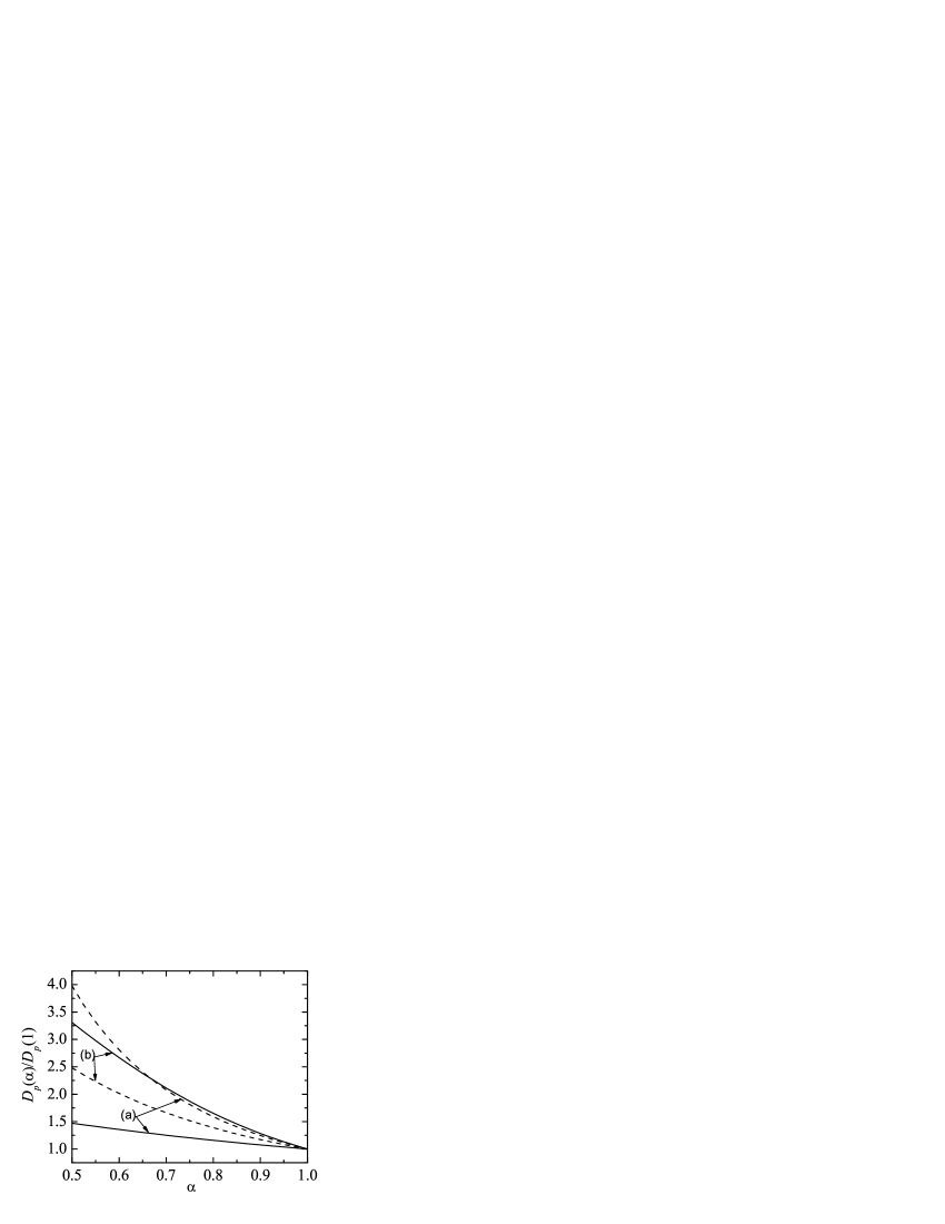
Figure 2: Plot of the reduced pressure diffusion coefficient $D_{p}(\alpha)/D_{p}(1)$ as a function of the (common) coefficient of restitution $\alpha$ for binary mixtures with $x_{1}=0.2$, $\omega=1$ in the case of a three-dimensional system ($d=3$) and two values of the mass ratio $\mu$: $\mu=0.5$ (a) and $\mu=4$ (b). The solid lines refer to the results derived here and the dashed lines correspond to the results assuming the equality of the partial temperatures.

Figure 3: Plot of the reduced thermal conductivity coefficient $\lambda(\alpha)/\lambda(1)$ as a function of the (common) coefficient of restitution $\alpha$ for binary mixtures with $x_{1}=0.2$, $\omega=1$ in the case of a three-dimensional system ($d=3$) and two values of the mass ratio $\mu$: $\mu=0.5$ (a) and $\mu=4$ (b). The solid lines refer to the results derived here and the dashed lines correspond to the results assuming the equality of the partial temperatures.

IV.5 Comparison with other theories

Before checking the accuracy of our expressions by comparing them with computer simulations, it is instructive first to make some comparison with previous results. mixture ; SGNT06 These results assume energy equipartition ($T_{i}=T$) and so, they are based on a standard CE expansion around the Maxwellian (32) instead of the local HCS distribution. Figures 2 and 3 show the dependence of the reduced pressure diffusion coefficient $D_{p}(\alpha)/D_{p}(1)$ and the reduced thermal conductivity coefficient $\lambda(\alpha)/\lambda(1)$, respectively, as a function of the (common) coefficient of restitution $\alpha_{ij}\equiv\alpha$ for $d=3$, $\omega=1$, $x_{1}=0.2$, and two different mass ratios $\mu$: $\mu=0.5$ (a) and $\mu=4$ (b). Here, $D_{p}(1)$ and $\lambda(1)$ are the values of $D_{p}$ and $\lambda$ for elastic collisions. We see that the deviation from the functional form for elastic collisions is quite important in both theories, even for moderate dissipation. It is apparent that the dependence of the transport coefficients on dissipation is quantitatively different in both models, especially at strong dissipation (say for instance, $\alpha=0.5$). This clearly shows the real quantitative effect of two different species temperatures on transport in granular mixtures.

V Comparison with Monte Carlo simulations

A said before, the expressions derived in Sec. IV for the NS transport coefficients have been obtained by considering two different approximations. First, since the deviation of $f_{i}^{(0)}$ from its Maxwellian form (28) is quite small in the region of thermal velocities, we have used the Maxwellian distribution (28) as a trial function for $f_{i}^{(0)}$. Second, we have only considered the leading terms of an expansion of the distribution $f_{i}^{(1)}$ in Sonine polynomials. Both approximations allow one to offer a simplified kinetic theory for a $d$-dimensional granular binary mixture. To check the accuracy of the above predictions, in this Section we numerically solve the Boltzmann equation by means of the DSMC method Bird and compare theory and simulation in the cases of the diffusion coefficient $D$ (in the tracer limit) and the shear viscosity coefficient $\eta$. Previous comparisons carried out for hard spheres GM04 ; MG03 when one takes into account the deviations of $f_{i}^{(0)}$ from their Maxwellian forms have shown good agreement between theory and simulation, even for strong dissipation (say $\alpha\gtrsim 0.5$). Here, we expect that such good agreement is also maintained in the case of hard disks when one replaces $f_{i}^{(0)}\to f_{i,M}$. Let us study each coefficient separately.

V.1 Tracer diffusion coefficient

We consider the special case in which one of the components of the mixture (say, for instance, species $1$) is present in tracer concentration ($x_{1}\to 0$). In this situation, $\partial\zeta^{*}/\partial x_{1}\to 0$ and so, the expression (50) for the reduced diffusion coefficient $D^{*}$ becomes

$$D^{*}=\frac{\gamma}{\nu^{*}-\frac{1}{2}\zeta^{*}},$$ (65)

where now

$$\zeta^{*}=\frac{\pi^{(d-1)/2}}{d\Gamma\left(d/2\right)}\left(\frac{\sigma_{2}}{\sigma_{12}}\right)^{d-1}\sqrt{2\mu_{12}}(1-\alpha_{22}^{2}),$$ (66)

$$\nu^{*}=\frac{2\pi^{(d-1)/2}}{d\Gamma\left(d/2\right)}\mu_{21}\sqrt{\mu_{12}+\mu_{21}\gamma}(1+\alpha_{12}).$$ (67)

The diffusion coefficient of impurities in a granular gas undergoing homogeneous cooling state can be measured in simulation from the mean square displacement of the tracer particle after a time interval $t$: M89 ; GM04

$$\frac{\partial}{\partial t}\langle|{\bf r}(t)-{\bf r}(0)|^{2}\rangle=\frac{2dD}{n_{2}}.$$ (68)

Equation (68) is the Einstein form. This relation (written in appropriate dimensionless variables to eliminate the time dependence of $D(t)$) was used in Ref. GM04, to measure the diffusion coefficient for hard spheres. More details on this procedure can be found in Ref. GM04, .

If the hydrodynamic description (or normal solution in the context of the CE method) applies, then the diffusion coefficient $D(t)$ depends on time only through its dependence on the temperature $T(t)$. In this case, after a transient regime, the reduced diffusion coefficient $D^{*}=(m_{1}m_{2}/\rho)D(t)\nu_{0}(t)/T(t)$ achieves a time-independent value. Here, we compare the steady state values of $D^{*}$ obtained from Monte Carlo simulations with the theoretical predictions given by the first Sonine approximation (65). The dependence of $D^{*}$ on the common coefficient of restitution $\alpha_{ij}\equiv\alpha$ is shown in Fig. 4 in the case of hard disks for three different systems. The symbols refer to computer simulations while the lines correspond to the kinetic theory results given by Eq. (65). Molecular dynamics (MD) results reported in Ref. BRCG00, when impurities and particles of the gas are mechanically equivalent have also been included. We observe that MD and DSMC results for $\mu=\omega=1$ are consistent among themselves in the range of values of $\alpha$ explored. This good agreement gives support to the applicability of the inelastic Boltzmann equation beyond the quasielastic limit. It is apparent that the agreement between the first Sonine approximation and simulation results is excellent when impurities and particles of the gas are mechanically equivalent and when impurities are much heavier and/or much larger than the particles of the gas (Brownian limit). However, some discrepancies between simulation an theory are found with decreasing values of the mass ratio $m_{1}/m_{2}$ and the size ratio $\sigma_{1}/\sigma_{2}$. These discrepancies are not easily observed in Fig. 4 because of the small magnitude of $D^{*}$ for $\mu=1/4$. The above findings agree with those previously reported for hard spheres, GM04 where it was shown that the second Sonine approximation improves the qualitative predictions from the first Sonine approximation for the cases in which the gas particles are heavier and/or larger than impurities. The comparison carried out here for disks confirms the above expectations and shows that the Sonine polynomial expansion exhibits a slow convergence for sufficiently small values of the mass ratio $\mu$ and/or the size ratio $\omega$.

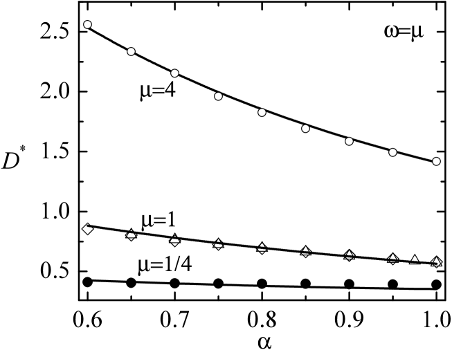
Figure 4: Plot of the reduced diffusion coefficient $D^{*}$ as a function of the (common) coefficient of restitution $\alpha$ for binary mixtures with $\omega=\mu$ in the case of a two-dimensional system ($d=2$). The symbols are computer simulation results obtained from the mean square displacement and the lines are the theoretical results obtained in the first Sonine approximation. The DSMC results correspond to $\mu=1/4$ ($\bullet$), $\mu=4$ ($\circ$) and $\mu=1$ ($\diamond$). Molecular dynamics results reported in Ref. BRCG00, for $\mu=1$ ($\triangle$) have also been included.

V.2 Shear viscosity coefficient

The shear viscosity $\eta$ is perhaps the most widely studied transport coefficient in granular fluids. In the case of granular mixtures, this coefficient has been measured MG03 when the system is heated by the action of an external driving force (thermostat) that exactly compensates for cooling effects associated with dissipation of collisions. The corresponding shear viscosity of the mixture (which slightly differs from the one obtained in the free cooling case) has been determined by means of the CE method in the low-density regime MG03 as well as for a moderate dense mixture. GM03 The theoretical predictions compare reasonably well with the corresponding numerical solutions of the Boltzmann and Enskog kinetic equations.

More recently, a new alternative method has been proposed to measure the (true) NS shear viscosity coefficient. MSG05 The method is based on the simple shear flow state modified by the introduction of a deterministic non-conservative force (which compensates for the collisional cooling) along with a stochastic process. While the external force is introduced to allow the granular fluid to approach a Newtonian regime, the stochastic process is introduced to mimic the conditions appearing in the CE method to NS order. Although the method was originally devised to a single granular gas, its extension to multicomponent systems is straightforward. Here, we use this procedure to measure the shear viscosity of the mixture by means of the DSMC method. More technical details on this procedure and its application to dense gases can be found in Ref. MSG05, .

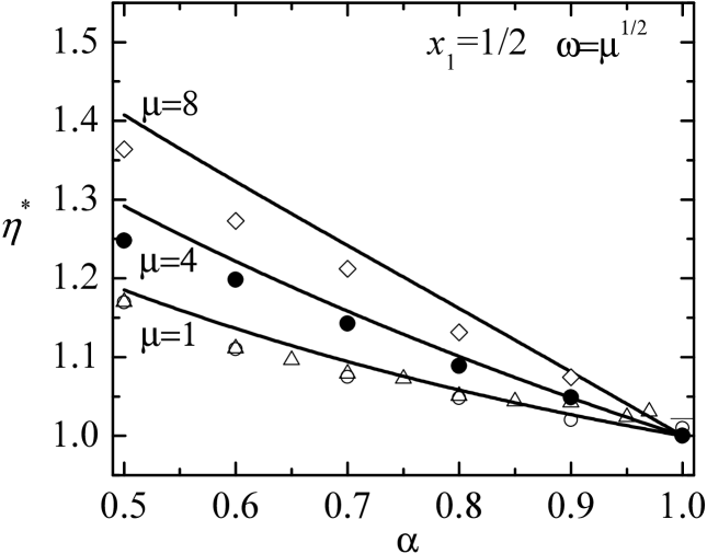
Figure 5: Plot of the reduced shear viscosity $\eta^{*}(\alpha)=\eta(\alpha)/\eta(1)$ as a function of the (common) coefficient of restitution $\alpha$ for binary mixtures constituted by particles of the same mass density ($\omega=\mu^{1/2}$) in the case of a two-dimensional system ($d=2$). The symbols are computer simulation results and the lines are the theoretical results obtained in the first Sonine approximation. The DSMC results correspond to $\mu=1$ ($\circ$), $\mu=4$ ($\bullet$) and $\mu=8$ ($\diamond$). We have also included DSMC results obtained in Ref. BRM04, for $\mu=1$ ($\triangle$) from the Green-Kubo relation.

Comparison between the first Sonine approximation and computer simulations for $\eta^{*}(\alpha)=\eta(\alpha)/\eta(1)$ is shown in Fig. 5 for three different mixtures constituted by particles of the same mass density (i.e., $\mu=\omega^{d}$) in the case of a two-dimensional system. Here, $\eta(1)$ refers to the elastic value for the shear viscosity coefficient and we have assumed again a common value of the coefficient of restitution $\alpha$. The symbols represent the simulation data and the lines correspond to the theoretical results. We have also included recent simulation results BRM04 for $\eta^{*}$ obtained from the Green-Kubo relation in the one-component case. Good agreement among the data presented here and those reported in Ref. BRM04, for $\mu=1$ is observed. In addition, as happens for hard spheres, MG03 we see that in general the agreement between the first Sonine approximation and simulation is quite good. At a quantitative level, the theory slightly overestimates the simulation data, especially for strong dissipation and for mixtures of particles of different masses and/or sizes. However, such discrepancies are quite small since for instance, they are smaller than 3% at $\alpha=0.5$ for $\mu=8$ and $\omega=\sqrt{8}$. This shows again the reliability of the first Sonine approximation for the shear viscosity coefficient. It must be noted that this conclusion cannot in principle be extended to the transport coefficients associated with the heat flux since recent comparisons for a single gas BRM04 ; BRMMG05 ; MSG06 have shown significant discrepancies between the first Sonine approximation and computer simulations for high inelasticity (say $\alpha\lesssim 0.7$). In this case, the agreement between theory and simulation can be significantly improved by the use of a modified first Sonine approximation. GSM06

VI Discussion

The main objective of this work has been to obtain the NS transport coefficients of a granular binary mixture at low density. In contrast to previous works, mixture ; SGNT06 the present study is based on a modified CE solution of the inelastic Boltzmann equation that takes into account non-equipartition of energy. There is no phenomenology involved as the equations and the transport coefficients have been derived systematically from the inelastic Boltzmann equation by the CE expansion around the local HCS. Since the spatial gradients are assumed to be independent of the coefficients of restitution, although the NS equations restrict their applicability to first order in gradients the corresponding transport coefficients hold a priori to arbitrary degree of inelasticity. All the calculations have been performed in an arbitrary number $d$ of dimensions, previous results GD02 being recovered for $d=3$.

The constitutive equations to NS order for the mass flux, the stress tensor, and the heat flux are given by Eqs. (33)–(35), respectively. The associated transport coefficients are the mutual diffusion coefficient $D$, the pressure diffusion coefficient $D_{p}$, and the thermal diffusion coefficient $D^{\prime}$ in the case of the mass flux, the shear viscosity coefficient $\eta$ for the pressure tensor, and the Dufour coefficient $D^{\prime\prime}$, the pressure energy coefficient $L$, and the thermal conductivity $\lambda$ in the case of the heat flux. These coefficients are determined from the solutions of the set of coupled linear integral equations (43b)–(46b). In addition, the NS transport coefficients also depend on the reference distributions $f_{i}^{(0)}$, which are not Maxwellians because they obey the integral equations (26). To solve the above integral equations and provide good estimates for the transport coefficients, we have considered two approximations: (i) the distributions $f_{i}^{(0)}$ have been replaced by their Maxwellian forms (28) at the temperature $T_{i}$ for that species and, (ii) we have only considered the leading terms in a series of Sonine polynomials for the first-order distribution $f_{i}^{(1)}$. By using both approximations, explicit expressions of the seven NS transport coefficients have been obtained as functions of the coefficients of restitution and the concentration and the ratios of mass and diameters. In dimensionless forms, the coefficients $D$, $D_{p}$, and $D^{\prime}$ are given by Eqs. (50)–(52), respectively, the shear viscosity $\eta$ is given by Eqs. (54) and (55), while the expressions of the coefficients $D^{\prime\prime}$, $L$, and $\lambda$ are provided by Eqs. (58)–(64).

Figure 6: Plot of the reduced shear viscosity coefficient $\eta^{*}=\eta(\alpha)/\eta(1)$ as a function of the (common) coefficient of restitution $\alpha$ for binary mixtures with $x_{1}=0.2$, $\omega=1$ and two values of the mass ratio $\mu$: $\mu=0.5$ (a) and $\mu=4$ (b). The solid lines refer to spheres ($d=3$) while the dashed lines correspond to disks ($d=2$).

Previous results mixture derived from the CE method have typically introduced additional assumptions for convenience that are not internally consistent with constructing a solution to the Boltzmann equation. Thus, in most of the cases the reference state $f_{i}^{(0)}$ has been chosen to be a Maxwellian at the same temperature [see Eq. (32)]. This assumption is presumed to give accurate results at weak dissipation where energy equipartition can be still considered as a good approximation. However, as shown in Fig. 1, the temperature ratio $T_{1}/T_{2}$ clearly differs from 1 as dissipation increases. Here, we have replaced $f_{i}^{(0)}\to f_{i,M}$ so that, the influence of the fourth-cumulants $c_{i}$ of $f_{i}^{(0)}$ has been ignored.GD99b Comparison between the expressions derived in this paper by taking the approximation (28) with those obtained by assuming energy equipartition shows important discrepancies as the coefficient of restitution decreases [see Figs. 2 and 3]. Moreover, as an added value of our theory, the use of the Maxwellian approximation (28) for $f_{i}^{(0)}$ allows one to provide simple and explicit expressions for all the transport coefficients in terms of the parameters of the mixture. This contrasts with the relatively recent study for hard spheres GD02 where the constitutive relations for the fluxes were not explicitly displayed.

As a complementary route and to check the reliability of our theory, the analytical results derived for the diffusion coefficient $D$ and the shear viscosity $\eta$ in the first Sonine approximation have been compared with those obtained from numerical solutions of the Boltzmann equation by means of the DSMC method for a two-dimensional system. For the sake of simplicity, all the simulations have considered a common coefficient of restitution $\alpha\equiv\alpha_{ij}$. As expected, theory and simulation clearly show that the influence of dissipation on mass and momentum transport is quite important since there is a relevant dependence of the diffusion $D$ and viscosity $\eta$ coefficients on $\alpha$. With respect to the accuracy of the theoretical predictions, we see that in general the CE results in the first Sonine approximation exhibit a good agreement with the simulation data. Exceptions to this agreement are extreme mass or size ratios and strong dissipation. These discrepancies are basically due to the use of the first Sonine approximation and can be partially mitigated by considering the second and third Sonine approximations GM04 or the use of a modified first Sonine approximation. GSM06

As said in the Introduction, the results obtained in this paper are of great practical interest since most of the experiments and simulations are performed in two dimensions. On the other hand, apart from this practical interest, the knowledge of the NS transport coefficients of a $d$-dimensional mixture allows one to investigate the influence of dimensionality on the transport properties of the system. To illustrate this effect, in Fig. 6 we plot the reduced shear viscosity $\eta^{*}\equiv\eta(\alpha)/\eta(1)$ versus the coefficient of restitution $\alpha$ for $\omega=1$, $x_{1}=0.2$, and two different mass ratios $\mu$: $\mu=0.5$ (a) and $\mu=4$ (b). We have considered the physical cases of hard spheres (solid lines) and hard disks (dashed lines). Although the qualitative dependence of $\eta^{*}$ on $\alpha$ is quite similar in both systems, we observe that the influence of dissipation on momentum transport is stronger for $d=3$ than for $d=2$. This trend is also observed in general in the remaining transport coefficients.

One of the main limitations of our theory is its restriction to dilute gases. In this situation, the collisional transfer contributions to the fluxes are neglected and only their kinetic contributions are considered. Possible extension of the present kinetic theory to higher densities can be done in the context of the revised Enskog theory. Preliminary results GM03 have been focused on the uniform shear flow state to get directly the shear viscosity coefficient. The extension of this study GM03 to states with gradients of concentration, pressure, and temperature is somewhat intricate due to subtleties associated with the spatial dependence of the pair correlations functions considered in the revised Enskog theory. On the other hand, it must be remarked that many of the collision integrals appearing in the Enskog description are the same as those appearing in the Boltzmann limit so that one can take advantage of the results reported in this paper. We plan to extend the results derived for moderately dense mixtures of smooth elastic hard spheres MCK83 to inelastic collisions in the near future.

Appendix A Chapman-Enskog method

The velocity distribution function $f_{1}^{(1)}$ obeys the equation

$$\left(\partial_{t}^{(0)}+{\cal L}_{1}\right)f_{1}^{(1)}+{\cal M}_{1}f_{2}^{(1)}=-\left(\partial_{t}^{(1)}+{\bf v}\cdot\nabla+{\bf g}\cdot\frac{\partial}{\partial{\bf v}}\right)f_{1}^{(0)}\;,$$ (69)

where the linear operators ${\cal L}_{1}$ and ${\cal M}_{1}$ are defined by Eqs. (47) and (48), respectively. A similar equation can be obtained for $f_{2}^{(1)}$ by interchanging $1\leftrightarrow 2$. The action of the time derivatives $\partial_{t}^{(1)}$ on the hydrodynamic fields is

$$D_{t}^{(1)}x_{1}=0,$$ (70)

$$D_{t}^{(1)}p=-\frac{d+2}{d}p\nabla\cdot{\bf u},$$ (71)

$$D_{t}^{(1)}T=-\frac{2T}{d}\nabla\cdot{\bf u},$$ (72)

$$D_{t}^{(1)}{\bf u}=-\rho^{-1}{\bf\nabla}p+{\bf g},$$ (73)

where $D_{t}^{(1)}=\partial_{t}^{(1)}+{\bf u\cdot\nabla}$ and use has been made of the results ${\bf j}_{i}^{(0)}={\bf q}^{(0)}=\zeta^{(1)}=0$. The last equality follows from the fact that the cooling rate is a scalar, and corrections to first order in the gradients can arise only from the divergence of a vector field. However, as is demonstrated below, there is no contribution to the distribution function proportional to this divergence. We note that this is special to the low density Boltzmann equation and such terms do occur at higher densities. GD99a Use of Eqs. (70)–(73) yields

$$-\left(\partial_{t}^{(1)}+{\bf v}\cdot\nabla+{\bf g}\cdot\frac{\partial}{\partial{\bf v}}\right)f_{1}^{(0)} = -\left(\frac{\partial}{\partial x_{1}}f_{1}^{(0)}\right)_{p,T}{\bf V}\cdot\nabla x_{1}-\left[f_{1}^{(0)}{\bf V}+\frac{nT}{\rho}\left(\frac{\partial}{\partial{\bf V}}f_{1}^{(0)}\right)\right]\cdot\nabla\ln p$$ (74)

$$+\left[f_{1}^{(0)}+\frac{1}{2}\frac{\partial}{\partial{\bf V}}\cdot\left({\bf V}f_{1}^{(0)}\right)\right]{\bf V}\cdot\nabla\ln T$$

$$+\left(V_{k}\frac{\partial}{\partial V_{\ell}}f_{1}^{(0)}-\frac{1}{d}\delta_{k\ell}{\bf V}\cdot\frac{\partial}{\partial{\bf V}}f_{1}^{(0)}\right)\nabla_{k}u_{\ell}.$$

Note that the external field does not appear in the right-hand side of Eq. (74). This is due to the particular form of the gravitational force. Using Eq. (74), Eq. (69) can be written as

$$\left(\partial_{t}^{(0)}+{\cal L}_{1}\right)f_{1}^{(1)}+{\cal M}_{1}f_{2}^{(1)}={\bf A}_{1}\cdot\nabla x_{1}+{\bf B}_{1}\cdot\nabla p+{\bf C}_{1}\cdot\nabla T+{\sf D}_{1}:\nabla{\bf u},$$ (75)

where

$${\bf A}_{i}({\bf V})=-\left(\frac{\partial}{\partial x_{1}}f_{i}^{(0)}\right)_{p,T}{\bf V},$$ (76)

$${\bf B}_{i}({\bf V})=-\frac{1}{p}\left[f_{i}^{(0)}{\bf V}+\frac{nT}{\rho}\left(\frac{\partial}{\partial{\bf V}}f_{i}^{(0)}\right)\right],$$ (77)

$${\bf C}_{i}({\bf V})=\frac{1}{T}\left[f_{i}^{(0)}+\frac{1}{2}\frac{\partial}{\partial{\bf V}}\cdot\left({\bf V}f_{i}^{(0)}\right)\right]{\bf V},$$ (78)

$${\sf D}_{i}({\bf V})={\bf V}\frac{\partial}{\partial{\bf V}}f_{i}^{(0)}-\frac{1}{d}\openone{\bf V}\cdot\frac{\partial}{\partial{\bf V}}f_{i}^{(0)}.$$ (79)

In Eqs. (76)–(79) it is understood that $i=1,2$ and $\openone$ is the unit tensor in $d$ dimensions. Note that the trace of ${\sf D}_{i}$ vanishes, confirming that the distribution function does not have contribution from the divergence of the flow field. The solutions to Eqs. (75) are of the form

$$f_{i}^{(1)}={\boldsymbol{\cal A}}_{i}\cdot\nabla x_{1}+{\boldsymbol{\cal B}}_{i}\cdot\nabla p+{\boldsymbol{\cal C}}_{i}\cdot\nabla T+{\cal D}_{i,k\ell}\nabla_{k}u_{\ell}\;.$$ (80)

The coefficients ${\boldsymbol{\cal A}}_{i}$, ${\boldsymbol{\cal B}}_{i}$, ${\boldsymbol{\cal C}}_{i}$, and ${\boldsymbol{\cal D}}_{i}$ are functions of the peculiar velocity ${\bf V}$ and the hydrodynamic fields. The cooling rate depends on space through its dependence on $x_{1}$, $p$, and $T$. The time derivative $\partial_{t}^{(0)}$ acting on these quantities can be evaluated by the replacement $\partial_{t}^{(0)}\rightarrow-\zeta^{(0)}\left(T\partial_{T}+p\partial_{p}\right)$. In addition, there are contributions from $\partial_{t}^{(0)}$ acting on the temperature and pressure gradients given by

$$\partial_{t}^{(0)}\nabla T = -\nabla\left(T\zeta^{(0)}\right)=-\zeta^{(0)}\nabla T-T\nabla\zeta^{(0)}$$ (81)

$$= -\frac{\zeta^{(0)}}{2}\nabla T-T\left[\left(\frac{\partial\zeta^{(0)}}{\partial x_{1}}\right)_{p,T}\nabla x_{1}+\frac{\zeta^{(0)}}{p}\nabla p\right],$$

$$\partial_{t}^{(0)}\nabla p = -\nabla\left(p\zeta^{(0)}\right)=-\zeta^{(0)}\nabla p-p\nabla\zeta^{(0)}$$ (82)

$$= -2\zeta^{(0)}\nabla p-p\left[\left(\frac{\partial\zeta^{(0)}}{\partial x_{1}}\right)_{p,T}\nabla x_{1}-\frac{\zeta^{(0)}}{2T}\nabla T\right].$$

The corresponding integral equations for the unknowns ${\boldsymbol{\cal A}}_{i}$, ${\boldsymbol{\cal B}}_{i}$, ${\boldsymbol{\cal C}}_{i}$, and ${\boldsymbol{\cal D}}_{i}$ are identified as the coefficients of the independent gradients in (80). This leads to Eqs. (43b)–(46b).

Appendix B Leading Sonine approximations

In this Appendix, we get the explicit expressions of the mass, momentum, and heat fluxes in the first Sonine approximation and neglecting the non-Gaussian corrections to the reference distributions $f_{i}^{(0)}$ (i.e., the cumulants $c_{i}=0$). The procedure to get the leading order contributions in the Sonine polynomial expansion to the transport coefficients is quite similar to the one previously used in the three-dimensional case. GD02 Only some partial results will be presented here.

B.1 Leading Sonine approximation to Mass Flux

In the case of the mass flux, the leading Sonine approximations (lowest degree polynomial) of the quantities ${\boldsymbol{\cal A}}_{i}$, ${\boldsymbol{\cal B}}_{i}$, ${\boldsymbol{\cal C}}_{i}$ are

$${\boldsymbol{\cal A}}_{1}({\bf V})\to-f_{1,M}{\bf V}\frac{m_{1}m_{2}n}{\rho n_{1}T_{1}}D,\quad{\boldsymbol{\cal A}}_{2}({\bf V})\to f_{2,M}{\bf V}\frac{m_{1}m_{2}n}{\rho n_{2}T_{2}}D$$ (83)

$${\boldsymbol{\cal B}}_{1}({\bf V})\to-f_{1,M}{\bf V}\frac{\rho}{pn_{1}T_{1}}D_{p},\quad{\boldsymbol{\cal B}}_{2}({\bf V})\to f_{2,M}{\bf V}\frac{\rho}{pn_{2}T_{2}}D_{p}$$ (84)

$${\boldsymbol{\cal C}}_{1}({\bf V})\to-f_{1,M}{\bf V}\frac{\rho}{Tn_{1}T_{1}}D^{\prime},\quad{\boldsymbol{\cal C}}_{2}({\bf V})\to f_{2,M}{\bf V}\frac{\rho}{Tn_{2}T_{2}}D^{\prime},$$ (85)

where $f_{i,M}$ are the Maxwellian distributions (28). Multiplication of Eqs. (43b)–(45b) by $m_{1}{\bf V}$ and integrating over the velocity yields

$$\left[-\zeta^{(0)}\left(T\partial_{T}+p\partial_{p}\right)+\nu\right]\left(-\frac{m_{1}m_{2}n}{\rho}D\right)=-\left(\frac{\partial}{\partial x_{1}}n_{1}T_{1}\right)_{p,T}-\rho\left(\frac{\partial\zeta^{(0)}}{\partial x_{1}}\right)_{p,T}\left(D_{p}+D^{\prime}\right),$$ (86)

$$\left[-\zeta^{(0)}\left(T\partial_{T}+p\partial_{p}\right)-2\zeta^{(0)}+\nu\right]\left(-\frac{\rho}{p}D_{p}\right)=-\frac{n_{1}T_{1}}{p}\left(1-\frac{m_{1}nT}{\rho T_{1}}\right)-\frac{\rho\zeta^{(0)}}{p}D^{\prime},$$ (87)

$$\left[-\zeta^{(0)}\left(T\partial_{T}+p\partial_{p}\right)-\frac{1}{2}\zeta^{(0)}+\nu\right]\left(-\frac{\rho}{T}D^{\prime}\right)=\frac{\rho\zeta^{(0)}}{2T}D_{p}.$$ (88)

Here, $\nu$ is the collision frequency defined by

$$\nu = \frac{1}{dn_{1}T_{1}}\int d{\bf V}_{1}m_{1}{\bf V}_{1}\cdot\left[{\cal L}_{1}(f_{1,M}{\bf V}_{1})-\delta\gamma{\cal M}_{1}(f_{2,M}{\bf V}_{2})\right]$$ (89)

$$= -\frac{1}{dn_{1}T_{1}}\int d{\bf V}_{1}m_{1}{\bf V}_{1}\cdot\left(J_{12}[{\bf v}_{1}|f_{1,M}{\bf V}_{1},f_{2}^{(0)}]-\delta\gamma J_{12}[{\bf v}_{1}|f_{1}^{(0)},f_{2,M}{\bf V}_{2}]\right),$$

where $\delta\equiv x_{1}/x_{2}$. The evaluation of the collision integral (89) is made in Appendix C. The self-collision terms of ${\cal L}_{i}$ arising from $J_{11}$ do not occur in Eq. (89) since they conserve momentum for species $1$. From dimensional analysis, $D\sim T^{1/2}$, $D_{p}\sim pT^{-1/2}$, and $D^{\prime}\sim pT^{-1/2}$ so the temperature and pressure derivatives can be performed in Eqs. (86)–(88). After performing them, one gets the expressions (50), (51), and (52) for the (reduced) coefficients $D^{*}$, $D_{p}^{*}$, and $D^{\prime\ast}$, respectively.

B.2 Leading Sonine approximation to Pressure Tensor

In the case of the pressure tensor, the leading Sonine approximation for the function ${\cal D}_{i,k\ell}$ is

$${\cal D}_{i,k\ell}({\bf V})\to-f_{i,M}({\bf V})\frac{\eta_{i}}{T}R_{i,k\ell}({\bf V}),\quad i=1,2$$ (90)

where

$$R_{i,k\ell}({\bf V})=m_{i}\left(V_{k}V_{\ell}-\frac{1}{d}V^{2}\delta_{k\ell}\right),$$ (91)

and

$$\eta_{i}=-\frac{1}{(d-1)(d+2)}\frac{T}{n_{i}T_{i}^{2}}\int d{\bf v}R_{i,k\ell}({\bf V}){\cal D}_{i,k\ell}({\bf V}).$$ (92)

The shear viscosity $\eta$ in this approximation can be written as

$$\eta=\frac{p}{\nu_{0}}\left(x_{1}\gamma_{1}^{2}\eta_{1}^{*}+x_{2}\gamma_{2}^{2}\eta_{2}^{*}\right),$$ (93)

where $\eta_{i}^{*}=\nu_{0}\eta_{i}$. The integral equations for the (reduced) coefficients $\eta_{i}^{*}$ are decoupled from the remaining transport coefficients. The two coefficients $\eta_{i}^{*}$ are obtained by multiplying Eqs. (46b) with $R_{i,k\ell}$ and integrating over the velocity to get the coupled set of equations

$$\left(\begin{array}[]{cc}\tau_{11}-\frac{1}{2}\zeta^{*}&\tau_{12}\\ \tau_{21}&\tau_{22}-\frac{1}{2}\zeta^{*}\end{array}\right)\left(\begin{array}[]{c}\eta_{1}^{*}\\ \eta_{2}^{*}\end{array}\right)=\left(\begin{array}[]{c}\gamma_{1}^{-1}\\ \gamma_{2}^{-1}\end{array}\right).$$ (94)

The (reduced) collision frequencies $\tau_{ij}$ are given in terms of the linear collision operator by

$$\tau_{ii}=\frac{1}{(d-1)(d+2)}\frac{1}{n_{i}T_{i}^{2}\nu_{0}}\int d{\bf v}_{1}R_{i,k\ell}{\cal L}_{i}\left(f_{i,M}R_{i,k\ell}\right),$$ (95)

$$\tau_{ij}=\frac{1}{(d-1)(d+2)}\frac{1}{n_{i}T_{i}^{2}\nu_{0}}\int d{\bf v}_{1}R_{i,k\ell}{\cal M}_{i}\left(f_{j,M}R_{j,k\ell}\right),\quad i\neq j.$$ (96)

The evaluation of these collision integrals is also given in Appendix C. The solution of Eq. (94) is elementary and yields Eq. (55).

B.3 Leading Sonine approximation to Heat Flux

The heat flux requires going up to the second Sonine approximation. In this case, the quantities ${\boldsymbol{\cal A}}_{i}$, ${\boldsymbol{\cal B}}_{i}$, ${\boldsymbol{\cal C}}_{i}$ are taken to be

$${\boldsymbol{\cal A}}_{1}({\bf V})\to f_{1,M}\left[-\frac{m_{1}m_{2}n}{\rho n_{1}T_{1}}D{\bf V}+d_{1}^{\prime\prime}{\bf S}_{1}({\bf V})\right],\quad{\boldsymbol{\cal A}}_{2}({\bf V})\to f_{2,M}\left[\frac{m_{1}m_{2}n}{\rho n_{2}T_{2}}D{\bf V}+d_{2}^{\prime\prime}{\bf S}_{2}({\bf V})\right]$$ (97)

$${\boldsymbol{\cal B}}_{1}({\bf V})\to f_{1,M}\left[-\frac{\rho}{pn_{1}T_{1}}D_{p}{\bf V}+\ell_{1}{\bf S}_{1}({\bf V})\right],\quad{\boldsymbol{\cal B}}_{2}({\bf V})\to f_{2,M}\left[\frac{\rho}{pn_{2}T_{2}}D_{p}{\bf V}+\ell_{2}{\bf S}_{2}({\bf V})\right]$$ (98)

$${\boldsymbol{\cal C}}_{1}({\bf V})\to f_{1,M}\left[-\frac{\rho}{Tn_{1}T_{1}}D^{\prime}{\bf V}+\lambda_{1}{\bf S}_{1}({\bf V})\right],\quad{\boldsymbol{\cal C}}_{2}({\bf V})\to f_{2,M}\left[\frac{\rho}{Tn_{2}T_{2}}D^{\prime}{\bf V}+\lambda_{2}{\bf S}_{2}({\bf V})\right],$$ (99)

where

$${\bf S}_{i}({\bf V})=\left(\frac{1}{2}m_{i}V^{2}-\frac{d+2}{2}T_{i}\right){\bf V}.$$ (100)

In these equations, it is understood that $D$, $D_{p}$ and $D^{\prime}$ are given by Eqs. (50), (51), and (52), respectively. The coefficients $d_{i}^{\prime\prime}$, $\ell_{i}$ and $\lambda_{i}$ are defined as

$$\left(\begin{array}[]{c}d_{i}^{\prime\prime}\\ \ell_{i}\\ \lambda_{i}\end{array}\right)=\frac{2}{d(d+2)}\frac{m_{i}}{n_{i}T_{i}^{3}}\int d{\bf v}\,{\bf S}_{i}({\bf V})\cdot\left(\begin{array}[]{c}{\boldsymbol{\cal A}}_{i}\\ {\boldsymbol{\cal B}}_{i}\\ {\boldsymbol{\cal C}}_{i}\end{array}\right).$$ (101)

These coefficients can be determined by multiplying Eqs. (43b)–(45b) (and their counterparts for the species 2) by ${\bf S}_{i}({\bf V})$ and integrating over the velocity. The final expressions can be obtained by taking into account that $d_{1}^{\prime\prime}\sim T^{-3/2}$, $\ell_{1}\sim T^{-3/2}/p$, and $\lambda_{1}\sim T^{-5/2}$ and the results

$$\int d{\bf v}\,m_{1}{\bf S}_{1}({\bf V})\cdot{\bf A}_{1}=-\frac{d(d+2)}{4}\frac{n_{1}T^{2}}{m_{1}}\left(\frac{\partial}{\partial x_{1}}\gamma_{1}^{2}\right)_{p,T},$$ (102)

$$\int d{\bf v}\,m_{1}{\bf S}_{1}({\bf V})\cdot{\bf B}_{1}=0,$$ (103)

$$\int d{\bf v}\,m_{1}{\bf S}_{1}({\bf V})\cdot{\bf C}_{1}=-\frac{d(d+2)}{2}\frac{n_{1}T_{1}^{2}}{m_{1}T}.$$ (104)

By using matrix notation, the coupled set of six equations for the quantities

$$\{d_{1}^{*},d_{2}^{*},\ell_{1}^{*},\ell_{2}^{*},\lambda_{1}^{*},\lambda_{2}^{*}\}$$ (105)

can be written as

$$\Lambda_{\sigma\sigma^{\prime}}X_{\sigma^{\prime}}=Y_{\sigma}.$$ (106)

Here, $d_{i}^{*}\equiv T\nu_{0}d_{i}^{\prime\prime}$, $\ell_{i}^{*}\equiv pT\nu_{0}\ell_{i}$, $\lambda_{i}^{*}\equiv T^{2}\nu_{0}\lambda_{i}$, $X_{\sigma^{\prime}}$ is the column matrix defined by the set (105) and $\Lambda_{\sigma\sigma^{\prime}}$ is the square matrix

$$\Lambda=\left(\begin{array}[]{cccccc}\nu_{11}-\frac{3}{2}\zeta^{*}&\nu_{12}&-\left(\frac{\partial\zeta^{*}}{\partial x_{1}}\right)_{p,T}&0&-\left(\frac{\partial\zeta^{*}}{\partial x_{1}}\right)_{p,T}&0\\ \nu_{21}&\nu_{22}-\frac{3}{2}\zeta^{*}&0&-\left(\frac{\partial\zeta^{*}}{\partial x_{1}}\right)_{p,T}&0&-\left(\frac{\partial\zeta^{*}}{\partial x_{1}}\right)_{p,T}\\ 0&0&\nu_{11}-\frac{5}{2}\zeta^{*}&\nu_{12}&-\zeta^{*}&0\\ 0&0&\nu_{21}&\nu_{22}-\frac{5}{2}\zeta^{*}&0&-\zeta^{*}\\ 0&0&\zeta^{*}/2&0&\nu_{11}-\zeta^{*}&\nu_{12}\\ 0&0&0&\zeta^{*}/2&\nu_{21}&\nu_{22}-\zeta^{*}\end{array}\right).$$ (107)

The column matrix ${\bf Y}$ is

$${\bf Y}=\left(\begin{array}[]{c}Y_{1}\\ Y_{2}\\ Y_{3}\\ Y_{4}\\ Y_{5}\\ Y_{6}\end{array}\right),$$ (108)

where note

$$Y_{1}=\frac{D^{*}}{x_{1}\gamma_{1}^{2}}\left(\omega_{12}-\zeta^{*}\right)-\frac{1}{\gamma_{1}^{2}}\left(\frac{\partial\gamma_{1}}{\partial x_{1}}\right)_{p,T},\quad Y_{2}=-\frac{D^{*}}{x_{2}\gamma_{2}^{2}}\left(\omega_{21}-\zeta^{*}\right)-\frac{1}{\gamma_{2}^{2}}\left(\frac{\partial\gamma_{2}}{\partial x_{1}}\right)_{p,T},$$ (109)

$$Y_{3}=\frac{D_{p}^{*}}{x_{1}\gamma_{1}^{2}}\left(\omega_{12}-\zeta^{*}\right),\quad Y_{4}=-\frac{D_{p}^{*}}{x_{2}\gamma_{2}^{2}}\left(\omega_{21}-\zeta^{*}\right),$$ (110)

$$Y_{5}=-\frac{1}{\gamma_{1}}+\frac{D^{\prime\ast}}{x_{1}\gamma_{1}^{2}}\left(\omega_{12}-\zeta^{*}\right),\quad Y_{6}=-\frac{1}{\gamma_{2}}-\frac{D^{\prime\ast}}{x_{2}\gamma_{2}^{2}}\left(\omega_{21}-\zeta^{*}\right).$$ (111)

Here, we have introduced the (reduced) collision frequencies

$$\nu_{ii}=\frac{2}{d(d+2)}\frac{m_{i}}{n_{i}T_{i}^{3}\nu_{0}}\int d{\bf v}_{1}{\bf S}_{i}\cdot{\cal L}_{i}\left(f_{i,M}{\bf S}_{i}\right),$$ (112)

$$\nu_{ij}=\frac{2}{d(d+2)}\frac{m_{i}}{n_{i}T_{i}^{3}\nu_{0}}\int d{\bf v}_{1}{\bf S}_{i}\cdot{\cal M}_{i}\left(f_{j,M}{\bf S}_{j}\right),\quad i\neq j,$$ (113)

$$\omega_{12}=\frac{2}{d(d+2)}\frac{m_{1}}{n_{1}T_{1}^{2}\nu_{0}}\left[\int d{\bf v}_{1}{\bf S}_{1}\cdot{\cal L}_{1}(f_{1,M}{\bf V}_{1})-\delta\gamma\int d{\bf v}_{1}{\bf S}_{1}\cdot{\cal M}_{1}(f_{2,M}{\bf V}_{2})\right],$$ (114)

$$\omega_{21}=\frac{2}{d(d+2)}\frac{m_{2}}{n_{2}T_{2}^{2}\nu_{0}}\left[\int d{\bf v}_{1}{\bf S}_{2}\cdot{\cal L}_{2}(f_{2,M}{\bf V}_{1})-\frac{1}{\delta\gamma}\int d{\bf v}_{1}{\bf S}_{2}\cdot{\cal M}_{2}(f_{1,M}{\bf V}_{2})\right].$$ (115)

The expressions of the collision integrals (112), (113), and (114) are given in Appendix C. The solution to Eq. (106) is

$$X_{\sigma}=\left(\Lambda^{-1}\right)_{\sigma\sigma^{\prime}}Y_{\sigma^{\prime}}.$$ (116)

From this relation one gets the expressions (61), (62), and (63) for the coefficients $d_{i}^{*}$, $\ell_{i}^{*}$ and $\lambda_{i}^{*}$, respectively.

Appendix C Collision integrals

In this Appendix we compute the different collision integrals appearing in the expressions of the transport coefficients. To simplify all the integrals, we use the property

$$\int d{\bf v}_{1}h({\bf V}_{1})J_{ij}\left[{\bf v}_{1}|f_{i},f_{j}\right]=\sigma_{ij}^{d-1}\int\,d{\bf v}_{1}\,\int\,d{\bf v}_{2}f_{i}({\bf V}_{1})f_{j}({\bf V}_{2})\int d\widehat{\boldsymbol{\sigma}}\,\Theta(\widehat{\boldsymbol{\sigma}}\cdot{\bf g}_{12})(\widehat{\boldsymbol{\sigma}}\cdot{\bf g}_{12})\,\left[h({\bf V}_{1}^{{}^{\prime\prime}})-h({\bf V}_{1})\right]\;,$$ (117)

with

$${\bf V}_{1}^{{}^{\prime\prime}}={\bf V}_{1}-\mu_{ji}(1+\alpha_{ij})(\widehat{\boldsymbol{\sigma}}\cdot{\bf g}_{12})\widehat{\boldsymbol{\sigma}}\;.$$ (118)

This result applies for both $i=j$ and $i\neq j$.

Let us start with the collision frequency $\nu$ defined by Eq. (89). Use of the identity (118) in (89) gives

$$\nu = \frac{m_{1}}{dn_{1}T_{1}}B_{3}\sigma_{12}^{d-1}\mu_{21}(1+\alpha_{12})\int\,d{\bf V}_{1}\,\int\,d{\bf V}_{2}\,g_{12}\left[f_{1,M}({\bf V}_{1})f_{2}^{(0)}({\bf V}_{2})({\bf V}_{1}\cdot{\bf g}_{12})\right.$$ (119)

$$\left.-\delta\gamma f_{1}^{(0)}({\bf V}_{1})f_{2,M}({\bf V}_{2})({\bf V}_{2}\cdot{\bf g}_{12})\right],$$

where use has been made of the result

$$\int d\widehat{\boldsymbol{\sigma}}\,\Theta(\widehat{{\boldsymbol{\sigma}}}\cdot{\bf g}_{12})\,(\widehat{\boldsymbol{\sigma}}\cdot{\bf g}_{12})^{k}\widehat{\boldsymbol{\sigma}}=B_{k+1}g_{12}^{k-1}{\bf g}_{12},$$ (120)

whith EB02

$$B_{k}\equiv\int d\widehat{\boldsymbol{\sigma}}\,\Theta(\widehat{{\boldsymbol{\sigma}}}\cdot{\bf g}_{12})\,(\widehat{\boldsymbol{\sigma}}\cdot{\widehat{\bf g}}_{12})^{k}=\pi^{(d-1)/2}\frac{\Gamma\left(\frac{k+1}{2}\right)}{\Gamma\left(\frac{k+d}{2}\right)}.$$ (121)

Substitution of the Maxwellian approximation (28) for $f_{i}^{(0)}$ gives

$$\nu=\frac{2}{d}\frac{\pi^{(d-1)/2}}{\Gamma\left(\frac{d+3}{2}\right)}\nu_{0}(1+\alpha_{12})\pi^{-d}\left(\theta_{1}\theta_{2}\right)^{d/2}\int\,d{\bf c}_{1}\,\int\,d{\bf c}_{2}\,y\,e^{-(\theta_{1}c_{1}^{2}+\theta_{2}c_{2}^{2})}\left[x_{2}\gamma_{1}^{-1}({\bf c}_{1}\cdot{\bf y})-x_{1}\gamma_{2}^{-1}({\bf c}_{2}\cdot{\bf y})\right],$$ (122)

where ${\bf c}_{i}\equiv{\bf V}_{i}/v_{0}$ and ${\bf y}\equiv{\bf c}_{1}-{\bf c}_{2}$. The integral can be performed by the change of variables $\{{\bf c}_{1},{\bf c}_{2}\}\to\{{\bf y},{\bf z}\}$, where ${\bf z}\equiv\theta_{1}{\bf c}_{1}+\theta_{2}{\bf c}_{2}$ and the Jacobian is $\left(\theta_{1}+\theta_{2}\right)^{-d}$. With this change, Eq. (122) becomes

$$\nu=\frac{2}{d}\frac{\pi^{(d-1)/2}}{\Gamma\left(\frac{d+3}{2}\right)}\nu_{0}(1+\alpha_{12})\pi^{-d}\left(\theta_{1}\theta_{2}\right)^{(d+1)/2}\left(\theta_{1}+\theta_{2}\right)^{-(1+d)}(x_{2}\mu_{21}+x_{1}\mu_{12})\int\,d{\bf y}\,\int\,d{\bf z}\,y^{3}e^{-(ay^{2}+bz^{2})},$$ (123)

where $a\equiv\theta_{1}\theta_{2}\left(\theta_{1}+\theta_{2}\right)^{-1}$ and $b\equiv\left(\theta_{1}+\theta_{2}\right)^{-1}$. The integral (123) can be easily computed and one directly gets the result (53) given in the text for the reduced collision frequency $\nu^{*}=\nu/\nu_{0}$.

The collision frequencies $\tau_{ij}$ defined by Eqs. (112) and (113) involve collision integrals of the form

$$\int d{\bf v}_{1}{\bf V}_{1}{\bf V}_{1}J_{ij}[f_{i},f_{j}]=\sigma_{ij}^{d-1}\int\,d{\bf v}_{1}\int\,d{\bf v}_{2}\,f_{i}({\bf V}_{1})f_{j}({\bf V}_{2})\int d\widehat{\boldsymbol{\sigma}}\,\Theta(\widehat{\boldsymbol{\sigma}}\cdot{\bf g}_{12})(\widehat{\boldsymbol{\sigma}}\cdot{\bf g}_{12})\,\left[{\bf V}_{1}^{\prime\prime}{\bf V}_{1}^{\prime\prime}-{\bf V}_{1}{\bf V}_{1}\right],$$ (124)

where the identity (117) has been used. The scattering rule (118) gives

$${\bf V}_{1}^{\prime\prime}{\bf V}_{1}^{\prime\prime}-{\bf V}_{1}{\bf V}_{1}=-\mu_{ji}(1+\alpha_{ij})(\widehat{\boldsymbol{\sigma}}\cdot{\bf g}_{12})\left[{\bf G}_{ij}\widehat{\boldsymbol{\sigma}}+\widehat{\boldsymbol{\sigma}}{\bf G}_{ij}+\mu_{ji}({\bf g}_{12}\widehat{\boldsymbol{\sigma}}+\widehat{\boldsymbol{\sigma}}{\bf g}_{12})-\mu_{ji}(1+\alpha_{ij})(\widehat{\boldsymbol{\sigma}}\cdot{\bf g}_{12})\widehat{\boldsymbol{\sigma}}\widehat{\boldsymbol{\sigma}}\right],$$ (125)

where ${\bf G}_{ij}=\mu_{ij}{\bf V}_{1}+\mu_{ji}{\bf V}_{2}$. Substitution of Eq. (125) into Eq. (124) allows the angular integral to be performed with the result

$$\int d\widehat{\boldsymbol{\sigma}}\,\Theta(\widehat{\boldsymbol{\sigma}}\cdot{\bf g}_{12})(\widehat{\boldsymbol{\sigma}}\cdot{\bf g}_{12}) \left[{\bf V}_{1}^{\prime\prime}{\bf V}_{1}^{\prime\prime}-{\bf V}_{1}{\bf V}_{1}\right]=-B_{3}m_{i}\mu_{ji}(1+\alpha_{ij})\left[g_{12}({\bf G}_{ij}{\bf g}_{12}+{\bf g}_{12}{\bf G}_{ij})\right.$$ (126)

$$\left.+3\frac{\mu_{ji}}{d+3}(1+\frac{2d}{3}-\alpha_{ij})g_{12}{\bf g}_{12}{\bf g}_{12}-\frac{\mu_{ji}}{d+3}(1+\alpha_{ij})g^{3}\openone\right].$$

Using (126) the integrals defining $\tau_{ij}$ can be calculated by the same mathematical steps as those made before for $\nu$. After a lengthy calculation, one gets

$$\int d{\bf v}_{1}R_{1,k\ell}J_{12}[f_{1}^{(0)},f_{2,M}R_{2,k\ell}] = -\frac{\pi^{(d-1)/2}}{2d\Gamma\left(\frac{d}{2}\right)}m_{1}m_{2}n_{1}n_{2}\mu_{21}(1+\alpha_{12})\sigma_{12}^{d-1}v_{0}^{5}\left(\theta_{1}\theta_{2}\right)^{-1/2}$$ (127)

$$\times \left\{2(d+3)(d-1)(\mu_{12}\theta_{2}-\mu_{21}\theta_{1})\theta_{2}^{-2}\left(\theta_{1}+\theta_{2}\right)^{-1/2}\right.$$

$$+3(d-1)\mu_{21}\left(1+\frac{2d}{3}-\alpha_{12}\right)\theta_{2}^{-2}\left(\theta_{1}+\theta_{2}\right)^{1/2}$$

$$\left.-\left[2d(d+1)-4\right]\theta_{2}^{-1}\left(\theta_{1}+\theta_{2}\right)^{-1/2}\right\},$$

$$\int d{\bf v}_{1}R_{1,k\ell}J_{12}[f_{1,M}R_{1,k\ell},f_{2}^{(0)}] = -\frac{\pi^{(d-1)/2}}{2d\Gamma\left(\frac{d}{2}\right)}m_{1}m_{2}n_{1}n_{2}\mu_{21}(1+\alpha_{12})\sigma_{12}^{d-1}v_{0}^{5}\left(\theta_{1}\theta_{2}\right)^{-1/2}$$ (128)

$$\times \left\{2(d+3)(d-1)(\mu_{12}\theta_{2}-\mu_{21}\theta_{1})\theta_{1}^{-2}\left(\theta_{1}+\theta_{2}\right)^{-1/2}\right.$$

$$+3(d-1)\mu_{21}\left(1+\frac{2d}{3}-\alpha_{12}\right)\theta_{1}^{-2}\left(\theta_{1}+\theta_{2}\right)^{1/2}$$

$$\left.+\left[2d(d+1)-4\right]\theta_{1}^{-1}\left(\theta_{1}+\theta_{2}\right)^{-1/2}\right\},$$

$$\int d{\bf v}_{1}R_{1,k\ell}\left\{J_{11}[f_{1}^{(0)},f_{1,M}R_{1,k\ell}]+J_{11}[f_{1,M}R_{1,k\ell},f_{1}^{(0)}]\right\} = -\frac{\pi^{(d-1)/2}}{\Gamma\left(\frac{d}{2}\right)}m_{1}^{2}n_{1}^{2}(1+\alpha_{11})\sigma_{1}^{d-1}(T_{1}/m_{1})^{5/2}$$ (129)

$$\times\frac{6(d-1)}{d}\left(1+\frac{2d}{3}-\alpha_{11}\right).$$

The corresponding expressions for $\tau_{ij}$ can be easily inferred from Eqs.  (127)–(129).

The collision frequencies $\nu_{ij}$ and $\omega_{ij}$ that determine the heat flux are defined by Eqs. (112), (113), and (114), respectively. To evaluate these collision integrals, one needs the partial results

$${\bf S}_{i}({\bf V}_{1}^{{}^{\prime\prime}})-{\bf S}_{i}({\bf V}_{1}) = \frac{m_{i}}{2}(1+\alpha_{ij})\mu_{ji}(\widehat{\boldsymbol{\sigma}}\cdot{\bf g}_{12})\left\{\left[(1-\alpha_{ij}^{2})\mu_{ji}^{2}(\widehat{\boldsymbol{\sigma}}\cdot{\bf g}_{12})^{2}-G_{ij}^{2}-\mu_{ji}^{2}g_{12}^{2}\right.\right.$$ (130)

$$\left.-2\mu_{ji}({\bf g}_{12}\cdot{\bf G}_{ij})+2(1+\alpha_{ij})\mu_{ji}(\widehat{\boldsymbol{\sigma}}\cdot{\bf g}_{12})(\widehat{\boldsymbol{\sigma}}\cdot{\bf G}_{ij})+(d+2)\frac{T_{i}}{m_{i}}\right]\widehat{\boldsymbol{\sigma}}$$

$$-\left[(1-\alpha_{ij})\mu_{ji}(\widehat{\boldsymbol{\sigma}}\cdot{\bf g}_{12})+2(\widehat{\boldsymbol{\sigma}}\cdot{\bf G}_{ij})\right]{\bf G}_{ij}$$

$$\left.-\mu_{ji}\left[(1-\alpha_{ij})\mu_{ji}(\widehat{\boldsymbol{\sigma}}\cdot{\bf g}_{12})+2(\widehat{\boldsymbol{\sigma}}\cdot{\bf G}_{ij})\right]{\bf g}_{12}\right\},$$

$$\int d\widehat{\boldsymbol{\sigma}}\,\Theta(\widehat{\boldsymbol{\sigma}}\cdot{\bf g}_{12})(\widehat{\boldsymbol{\sigma}}\cdot{\bf g}_{12}) \left[{\bf S}_{i}({\bf V}_{1}^{{}^{\prime\prime}})-{\bf S}_{i}({\bf V}_{1})\right]=-\frac{m_{i}}{2}\frac{\pi^{(d-1)/2}}{\Gamma\left(\frac{d+3}{2}\right)}(1+\alpha_{ij})\mu_{ji}$$ (131)

$$\times\left\{\left[g_{12}G_{ij}^{2}+\mu_{ji}^{2}\frac{4\alpha_{ij}^{2}-(d+3)\alpha_{ij}+2(d+1)}{d+3}g_{12}^{3}\right.\right.$$

$$\left.-2\mu_{ji}\frac{3\alpha_{ij}-2d-3}{d+3}g_{12}\left({\bf g}_{12}\cdot{\bf G}_{ij}\right)-(d+2)\frac{T_{i}}{m_{i}}g_{12}\right]{\bf g}_{12}$$

$$\left.+\left[2g_{12}\left({\bf g}_{12}\cdot{\bf G}_{ij}\right)-\mu_{ji}\frac{(d+5)\alpha_{ij}-d-1}{d+3}g_{12}^{3}\right]{\bf G}_{ij}\right\}\;.$$

The integrals $\omega_{ij}$ and $\nu_{ij}$ can be explicitly evaluated by using (131) and the same mathematical steps as before. After a lengthy algebra, one gets

$$\omega_{12} = \frac{\pi^{(d-1)/2}}{\Gamma\left(\frac{d}{2}\right)}\frac{2}{d\sqrt{2}}\left(\frac{\sigma_{1}}{\sigma_{12}}\right)^{d-1}x_{1}\theta_{1}^{-1/2}(1-\alpha_{11}^{2})$$ (132)

$$+\frac{\pi^{(d-1)/2}}{\Gamma\left(\frac{d}{2}\right)}\frac{2}{d(d+2)}x_{1}\mu_{21}(1+\alpha_{12})(\theta_{1}+\theta_{2})^{-1/2}\theta_{1}^{1/2}\theta_{2}^{-3/2}\left(\frac{x_{2}}{x_{1}}A-\gamma B\right),$$

$$\nu_{11} = \frac{\pi^{(d-1)/2}}{\Gamma\left(\frac{d}{2}\right)}\frac{8}{d(d+2)}\left(\frac{\sigma_{1}}{\sigma_{12}}\right)^{d-1}x_{1}(2\theta_{1})^{-1/2}(1+\alpha_{11})\left[\frac{d-1}{2}+\frac{3}{16}(d+8)(1-\alpha_{11})\right]$$ (133)

$$+\frac{\pi^{(d-1)/2}}{\Gamma\left(\frac{d}{2}\right)}\frac{1}{d(d+2)}x_{2}\mu_{21}(1+\alpha_{12})\left(\frac{\theta_{1}}{\theta_{2}(\theta_{1}+\theta_{2})}\right)^{3/2}\left[E-(d+2)\frac{\theta_{1}+\theta_{2}}{\theta_{1}}A\right],$$

$$\nu_{12}=-\frac{\pi^{(d-1)/2}}{\Gamma\left(\frac{d}{2}\right)}\frac{1}{d(d+2)}x_{2}\frac{\mu_{21}^{2}}{\mu_{12}}(1+\alpha_{12})\left(\frac{\theta_{1}}{\theta_{2}(\theta_{1}+\theta_{2})}\right)^{3/2}\left[F+(d+2)\frac{\theta_{1}+\theta_{2}}{\theta_{2}}B\right].$$ (134)

In the above equations we have introduced the quantities note

$$A = (d+2)(2\beta_{12}+\theta_{2})+\mu_{21}(\theta_{1}+\theta_{2})\left\{(d+2)(1-\alpha_{12})-[(11+d)\alpha_{12}-5d-7]\beta_{12}\theta_{1}^{-1}\right\}$$

$$+3(d+3)\beta_{12}^{2}\theta_{1}^{-1}+2\mu_{21}^{2}\left(2\alpha_{12}^{2}-\frac{d+3}{2}\alpha_{12}+d+1\right)\theta_{1}^{-1}(\theta_{1}+\theta_{2})^{2}-(d+2)\theta_{2}\theta_{1}^{-1}(\theta_{1}+\theta_{2}),$$

$$B = (d+2)(2\beta_{12}-\theta_{1})+\mu_{21}(\theta_{1}+\theta_{2})\left\{(d+2)(1-\alpha_{12})+[(11+d)\alpha_{12}-5d-7]\beta_{12}\theta_{2}^{-1}\right\}$$

$$-3(d+3)\beta_{12}^{2}\theta_{2}^{-1}-2\mu_{21}^{2}\left(2\alpha_{12}^{2}-\frac{d+3}{2}\alpha_{12}+d+1\right)\theta_{2}^{-1}(\theta_{1}+\theta_{2})^{2}+(d+2)(\theta_{1}+\theta_{2}),$$

$$E = 2\mu_{21}^{2}\theta_{1}^{-2}(\theta_{1}+\theta_{2})^{2}\left(2\alpha_{12}^{2}-\frac{d+3}{2}\alpha_{12}+d+1\right)\left[(d+2)\theta_{1}+(d+5)\theta_{2}\right]$$

$$-\mu_{21}(\theta_{1}+\theta_{2})\left\{\beta_{12}\theta_{1}^{-2}[(d+2)\theta_{1}+(d+5)\theta_{2}][(11+d)\alpha_{12}-5d-7]\right.$$

$$\left.-\theta_{2}\theta_{1}^{-1}[20+d(15-7\alpha_{12})+d^{2}(1-\alpha_{12})-28\alpha_{12}]-(d+2)^{2}(1-\alpha_{12})\right\}$$

$$+3(d+3)\beta_{12}^{2}\theta_{1}^{-2}[(d+2)\theta_{1}+(d+5)\theta_{2}]+2\beta_{12}\theta_{1}^{-1}[(d+2)^{2}\theta_{1}+(24+11d+d^{2})\theta_{2}]$$

$$+(d+2)\theta_{2}\theta_{1}^{-1}[(d+8)\theta_{1}+(d+3)\theta_{2}]-(d+2)(\theta_{1}+\theta_{2})\theta_{1}^{-2}\theta_{2}[(d+2)\theta_{1}+(d+3)\theta_{2}],$$

$$F = 2\mu_{21}^{2}\theta_{2}^{-2}(\theta_{1}+\theta_{2})^{2}\left(2\alpha_{12}^{2}-\frac{d+3}{2}\alpha_{12}+d+1\right)\left[(d+5)\theta_{1}+(d+2)\theta_{2}\right]$$

$$-\mu_{21}(\theta_{1}+\theta_{2})\left\{\beta_{12}\theta_{2}^{-2}[(d+5)\theta_{1}+(d+2)\theta_{2}][(11+d)\alpha_{12}-5d-7]\right.$$

$$\left.+\theta_{1}\theta_{2}^{-1}[20+d(15-7\alpha_{12})+d^{2}(1-\alpha_{12})-28\alpha_{12}]+(d+2)^{2}(1-\alpha_{12})\right\}$$

$$+3(d+3)\beta_{12}^{2}\theta_{2}^{-2}[(d+5)\theta_{1}+(d+2)\theta_{2}]-2\beta_{12}\theta_{2}^{-1}[(24+11d+d^{2})\theta_{1}+(d+2)^{2}\theta_{2}]$$

$$+(d+2)\theta_{1}\theta_{2}^{-1}[(d+3)\theta_{1}+(d+8)\theta_{2}]-(d+2)(\theta_{1}+\theta_{2})\theta_{2}^{-1}[(d+3)\theta_{1}+(d+2)\theta_{2}].$$

Here, $\beta_{12}=\mu_{12}\theta_{2}-\mu_{21}\theta_{1}$. From Eqs. (132)–(C), one easily gets the expressions for $\omega_{21}$, $\nu_{22}$ and $\nu_{21}$ by interchanging $1\leftrightarrow 2$.

In the case of a three-dimensional system ($d=3$), all the above results reduce to those previously obtained for hard spheres when one takes Maxwellian distributions for the reference homogeneous cooling state. GD02 ; MGD06

References

- (1) A. Goldshtein and M. Shapiro, Mechanics of collisional motion of granular materials. Part 1. General hydrodynamic equations, J. Fluid Mech. 282:75–114 (1995).
- (2) J. J. Brey, J. W. Dufty, and A. Santos, Dissipative dynamics for hard spheres, J. Stat. Phys. 87:1051–1066 (1997).
- (3) N. V. Brilliantov and T. Pöschel, Kinetic Theory of Granular Gases (Oxford University Press, Oxford, 2004).
- (4) S. Chapman and T. G. Cowling, The Mathematical Theory of Nonuniform Gases (Cambridge University Press, Cambridge, 1970).
- (5) J. J. Brey, J. W. Dufty, C. S. Kim, and A. Santos, Hydrodynamics for granular flow at low-density, Phys. Rev. E 58:4638–4653 (1998); J. J. Brey and D. Cubero, Hydrodynamic transport coefficients of granular gases, in Granular Gases, edited by T. Pöschel and S. Luding, Lecture Notes in Physics (Springer Verlag, Berlin, 2001), pp. 59–78; V. Garzó and J. M. Montanero, Transport coefficients of a heated granular gas, Physica A 313:336–356 (2002).
- (6) J. T. Jenkins and F. Mancini, Kinetic theory for binary mixtures of smooth, nearly elastic spheres, Phys. Fluids A 1:2050–2057 (1989); P. Zamankhan, Kinetic theory for multicomponent dense mixtures of slightly inelastic spherical particles, Phys. Rev. E 52:4877–4891 (1995); B. Arnarson and J. T. Willits, Thermal diffusion in binary mixtures of smooth, nearly elastic spheres with and without gravity, Phys. Fluids 10:1324–1328 (1998); J. T. Willits and B. Arnarson, Kinetic theory of a binary mixture of nearly elastic disks, Phys. Fluids 11:3116–3122 (1999).
- (7) V. Garzó and J. W. Dufty, Homogeneous cooling state for a granular mixture, Phys. Rev. E 60:5706–5713 (1999).
- (8) P. A. Martin and J. Piasecki, Thermalization of a particle by dissipative collisions, Europhys. Lett. 46:613–616 (1999).
- (9) See for instance, J. M. Montanero and V. Garzó, Monte Carlo simulation of the homogeneous cooling state for a granular mixture, Gran. Matt. 4:17–24 (2002); A. Barrat and E. Trizac, Lack of energy equipartition in homogeneous heated binary granular mixtures, ibid. 4:57–63 (2002); S. R. Dahl, C. M. Hrenya, V. Garzó, and J. W. Dufty, Kinetic temperatures for a granular mixture, Phys. Rev. E 66:041301 (2002); R. Pagnani, U. M. B. Marconi, and A. Puglisi, Driven low density granular mixtures, ibid. 66:051304 (2002); D. Paolotti, C. Cattuto, U. M. B. Marconi, and A. Puglisi, Dynamical properties of vibrofluidized granular mixtures, Gran. Matt. 5:75–83 (2003); P. Krouskop and J. Talbot, Mass and size effects in three-dimensional vibrofluidized granular mixtures, Phys. Rev. E 68: 021304 (2003); H. Wang, G. Jin, and Y. Ma, Simulation study on kinetic temperatures of vibrated binary granular mixtures, ibid. 68:031301 (2003); J. J. Brey, M. J. Ruiz-Montero, and F. Moreno, Energy partition and segregation for an intruder in a vibrated granular system under gravity, Phys. Rev. Lett. 95:098001 (2005); M. Schröter, S. Ulrich , J. Kreft , J. B. Swift, and H. L. Swinney, Mechanisms in the size segregation of a binary granular mixture, Phys. Rev. E 74:011307 (2006).
- (10) R. D. Wildman and D. J. Parker, Coexistence of two granular temperatures in binary vibrofluidized beds, Phys. Rev. Lett. 88:064301 (2002); K. Feitosa and N. Menon, Breakdown of energy equipartition in a 2D binary vibrated granular gas, ibid. 88:198301 (2002).
- (11) J. Jenkins and F. Mancini, Balance laws and constitutive relations for plane flows of a dense binary mixture of smooth, nearly elastic, circular disks, J. Appl. Mech. 54:27–34 (1987).
- (12) V. Garzó and J. W. Dufty, Hydrodynamics for a granular binary mixture at low density, Phys. Fluids 14:1476–1490 (2002).
- (13) V. Garzó and A. Astillero, Transport coefficients for inelastic Maxwell mixtures, J. Stat. Phys. 118:935–971 (2005).
- (14) V. Garzó, J. M. Montanero, and J. W. Dufty, Mass and heat fluxes for a binary granular mixture at low-density, Phys. Fluids 18:083305 (2006).
- (15) V. Garzó and J. M. Montanero, Diffusion of impurities in a granular gas, Phys. Rev. E 69: 021301 (2004).
- (16) J. M. Montanero and V. Garzó, Shear viscosity for a heated granular binary mixture at low-density, Phys. Rev. E 67:021308 (2003).
- (17) D. Serero, I. Goldhirsch, S. H. Noskowicz, and M.-L. Tan, Hydrodynamics of granular gases and granular gas mixtures, J. Fluid Mech. 554:237–258 (2006).
- (18) See for instance, S. Warr, J. M. Huntley, and G. T. H. Jacques, Fluidization of a two-dimensional granular system: Experimental study and scaling behavior, Phys. Rev. E 52:5583–5595 (1995); J. S. Olafsen and J. S. Urbach, Velocity distribution and density fluctuations in a granular gas, ibid. 60:R2468–R2471 (1999); R. D. Wildman, J. M. Huntley, and J. P. Hansen, Self-diffusion of grains in two-dimensional vibrofluidized bed, ibid. 60:7066–7075 (1999); F. Rouyer and N. Menon, Velocity fluctuations in a homogeneous 2D granular gas in steady state, Phys. Rev. Lett. 85:3676–3679 (2000); D. L. Blair and A. Kudrolli, Velocity correlations in dense granular flows, Phys. Rev. E 64:050301 (2001); S. Horluck, M. van Hecke, and P. Dimon, Shock waves in two-dimensional granular flow: Effects of rough walls and polydispersity, ibid. 67:021304 (2003).
- (19) G. A. Bird, Molecular Gas Dynamics and the Direct Simulation Monte Carlo of Gas Flows (Clarendon, Oxford, 1994).
- (20) A. Santos, V. Garzó, and J. W. Dufty, Inherent rheology of a granular fluid in uniform shear flow, Phys. Rev. E 69:061303 (2004).
- (21) T. P. C. van Noije and M. H. Ernst, Velocity distributions in inhomogeneous granular fluids: the free and the heated case, Gran. Matt. 1:57–64(1998).
- (22) V. Garzó, Tracer diffusion in granular shear flows, Phys. Rev. E 66:021308 (2002).
- (23) J. J. Brey, M. J. Ruiz-Montero, and F. Moreno, Energy partition and segregation for an intruder in a vibrated granular system under gravity, Phys. Rev. Lett. 95:098001 (2005); Hydrodynamic profiles for an impurity in an open vibrated granular gas, Phys. Rev. E 73:031301 (2006).
- (24) J. J. Brey and D. Cubero, Hydrodynamic transport coefficients of granular gases, in Granular Gases, edited by T. Pöschel and S. Luding, Lecture Notes in Physics (Springer Verlag, Berlin, 2001), pp. 59–78.
- (25) J. A. McLennan, Introduction to Nonequilibrium Statistical Mechanics (Prentice-Hall, New Jersey, 1989).
- (26) J. J. Brey, M. J. Ruiz-Montero, D. Cubero, and R. García-Rojo, Self-diffusion in freely evolving granular gases, Phys. Fluids 12:876–883 (2000).
- (27) V. Garzó and J. M. Montanero, Shear viscosity for a moderately dense granular binary mixture, Phys. Rev. E 68:041302 (2003).
- (28) J. M. Montanero, A. Santos, and V. Garzó, DSMC evaluation of the Navier-Stokes shear viscosity of a granular fluid, in Rarefied Gas Dynamics 24, edited by M. Capitelli (American Institute of Physics, Vol. 762, 2005), pp. 797–802; preprint arXiv: cond-mat/0411219.
- (29) J. J. Brey and M. J. Ruiz-Montero, Simulation study of the Green-Kubo relations for dilute granular gases, Phys. Rev. E 70:051301 (2004).
- (30) J. J. Brey, M. J. Ruiz-Montero, P. Maynar, and M. I. García de Soria, Hydrodynamic modes, Green-Kubo relations, and velocity correlations in dilute granular gases, J. Phys.: Condens. Matter 17:S2489–S2502 (2005).
- (31) J. M. Montanero, A. Santos, and V. Garzó, First-order Chapman-Enskog velocity distribution function in a granular gas, Physica A 376:75–93 (2007).
- (32) V. Garzó, A. Santos, and J. M. Montanero, Modified Sonine approximation for the Navier-Stokes transport coefficients of a granular gas, Physica A 376:94–107 (2007).
- (33) M. López de Haro, E. G. D. Cohen, and J. M. Kincaid, The Enskog theory for multicomponent mixtures. I. Linear transport theory, J. Chem. Phys. 78:2746–2759 (1983).
- (34) V. Garzó and J. W. Dufty, Dense fluid transport for inelastic hard spheres, Phys. Rev. E 59:5895–5911 (1999).
- (35) M. H. Ernst and R. Brito, Scaling solutions of inelastic Boltzmann equations with over-populated high energy tails, J. Stat. Phys. 109:407–432 (2002).
- (36) Some misprints occur in the expressions given in Ref. GD02, for the heat flux. The results displayed here correct and extend such results to dimensions.