Localized vibrational modes in optically bound structures

Jack Ng and C.T. Chan

Department of Physics, Hong Kong University of Science and Technology, Clearwater Bay, Hong Kong, China

Abstract

We show, through analytical theory and rigorous numerical calculations, that optical binding can organize a collection of particles into stable one-dimensional lattice. This lattice, as well as other optically-bound structures, are shown to exhibit spatially localized vibrational eigenmodes. The origin of localization here is distinct from the usual mechanisms such as disorder, defect, or nonlinearity, but is a consequence of the long-ranged nature of optical binding. For an array of particles trapped by an interference pattern, the stable configuration is often dictated by the external light source, but our calculation revealed that inter-particle optical binding forces can have a profound influence on the dynamics.

OCIS codes:  140.7010,220.4610,220.4880,999.9999(Optical Binding)

Since its introduction many years ago,[1] optical manipulation has evolved into a major technique for manipulating small particles, and recently, simultaneous manipulations of multi-particles have been demonstrated.[2]It is known that in addition to the well-known one-body force such as the gradient force that depends on the intensity profile, there is an optical binding (OB) force that couples the particles together.[3]^,[4] Nevertheless, for an extended array of particles, the nature of OB is not fully understood, although some theoretical efforts were devoted to small clusters.[4]^,[5] As the principles underlining these inter-particle forces are different from that of the traditional light-trapping, we expect some new and interesting applications.

In this paper, we demonstrate an interesting consequence of OB in a spatially extended structure bound by light: the existence of spatially localized VEM (vibrational eigenmodes). We illustrate the physics by considering a one-dimensional “lattice” bound by light. Wave localization is known to occur in defect or impurity sites of an otherwise ordered lattice. In solids, the “defect” can be impurity atoms that localize phonons, and in the intrinsic localized modes, the “defect” is derived from the nonlinearly excited particles.[6] Here the localization occurs in the linear dynamics regime in an ordered array of identical particles without defect or disorder.

Optically bound structures have been investigated in a number of recent experiments. Stable cluster configurations had been realized[4]^,[7]^,[8]^,[9]^,[10]^,[11] and vibrational motions were observed.[7] In particular, the most commonly observed geometry is an one-dimensional array of particles, bound by a pair counterpropagating beams[7]^,[8]^,[9] or evanescent waves.[10]^,[11]

Consider a linear chain of $N$ evenly spaced spheres in air. The particles have mass density $\rho$=1,050 kg/m³, dielectric constant $\varepsilon$=2.53 ($\sim$polystyrene), and radii $a=\lambda/10=52$ nm, so that they are small compare to the incident light’s wavelength $\lambda$=520 nm. The particles are illuminated by the standing wave formed by a pair of counterpropagating plane waves

$$\mathord{\buildrel\lower 3.0pt\hbox{$\scriptscriptstyle\rightharpoonup$}\over{E}}_{in}(\mathord{\buildrel\lower 3.0pt\hbox{$\scriptscriptstyle\rightharpoonup$}\over{r}})=2E_{0}\cos\left({kz}\right)\hat{x},$$ (1)

where $k$ is the wavenumber, and the intensity for each beam is set to be 0.01 W/$\mu$m².[3]^,[4]

To calculate the optical force acting on the particles, we employ the rigorous and highly accurate multiple scattering and Maxwell stress tensor (MS-MST) formalism,[4] which requires no approximation and subject only to numerical truncation errors (we use multipoles up to $L$=6). The optical force tends to drive small particles to the region of strong light intensity. For an array of $N$ evenly spaced particles aligned along the $z$-axis, one expects a stable one-dimensional lattice with a lattice constant of $\lambda$/2:

$${\begin{array}[]{*{20}c}{\mathord{\buildrel\lower 3.0pt\hbox{$\scriptscriptstyle\rightharpoonup$}\over{R}}_{n}=\left({0,0,n\lambda/2}\right),\hfill}&{n=1,2\ldots,N\hfill}\\ \end{array}},$$ (2)

where $\mathord{\buildrel\lower 3.0pt\hbox{$\scriptscriptstyle\rightharpoonup$}\over{R}}_{n}$ is the equilibrium position for the n-th particle. Indeed, we found that the geometry defined in (2) corresponds to a zero-force configuration and the configuration is proven to be stable by using linear stability analysis.[4]^,[12] The longitudinal trapping (along the $z$-axis) is mainly provided by the gradient force of the incident beam, and it is further enhanced by OB.[13] On the other hand, the transverse stability (on the xy-plane) is solely induced by OB. We note that there are other beam configurations, other than that specified by (1), that can stabilize a linear chain as demonstrated by recent experiments.[7]^,[8]^,[11]^,[14]

The VEMs are obtained by diagonalizing the force matrix $(\mathord{\buildrel\lower 3.0pt\hbox{$\scriptscriptstyle\leftrightarrow$}\over{K}})_{jk}=\partial(\mathord{\buildrel\lower 3.0pt\hbox{$\scriptscriptstyle\rightharpoonup$}\over{f}}_{light})_{j}/\partial(\Delta\mathord{\buildrel\lower 3.0pt\hbox{$\scriptscriptstyle\rightharpoonup$}\over{x}})_{k}$,[4] which is found by linearizing the optical force near the equilibrium: $\mathord{\buildrel\lower 3.0pt\hbox{$\scriptscriptstyle\rightharpoonup$}\over{f}}_{light}\approx\mathord{\buildrel\lower 3.0pt\hbox{$\scriptscriptstyle\leftrightarrow$}\over{K}}\Delta\mathord{\buildrel\lower 3.0pt\hbox{$\scriptscriptstyle\rightharpoonup$}\over{x}}$, where $\Delta\mathord{\buildrel\lower 3.0pt\hbox{$\scriptscriptstyle\rightharpoonup$}\over{x}}$ is the displacement vector of the i-th particle away from its equilibrium configuration. The vibration profile of the VEM is described by the eigenvectors $\mathord{\buildrel\lower 3.0pt\hbox{$\scriptscriptstyle\rightharpoonup$}\over{V}}^{(i)}$ of $\mathord{\buildrel\lower 3.0pt\hbox{$\scriptscriptstyle\leftrightarrow$}\over{K}}$, and the natural vibrational frequency is $\Omega_{0i}=(-K_{i}/m)^{1/2}$ where $K_{i}$ is an eigenvalue of $\mathord{\buildrel\lower 3.0pt\hbox{$\scriptscriptstyle\leftrightarrow$}\over{K}}$ and $m$ is the mass of a sphere. Due to the reflection symmetry, the modes fall into three separate branches (each of $N$ modes), corresponding to the vibrations along the three Cartesian directions (see Fig. 1(e)). We shall denote the branches as the $\mathord{\buildrel\lower 3.0pt\hbox{$\scriptscriptstyle\rightharpoonup$}\over{k}}$-branch, $\mathord{\buildrel\lower 3.0pt\hbox{$\scriptscriptstyle\rightharpoonup$}\over{E}}$-branch, and $(\mathord{\buildrel\lower 3.0pt\hbox{$\scriptscriptstyle\rightharpoonup$}\over{k}}\times\mathord{\buildrel\lower 3.0pt\hbox{$\scriptscriptstyle\rightharpoonup$}\over{E}})$-branch, corresponding respectively to particle displacements along the incident wavevector$\mathord{\buildrel\lower 3.0pt\hbox{$\scriptscriptstyle\rightharpoonup$}\over{k}}=\pm k\hat{z}$, the incident polarization ($x$-axis), and the $y$-axis.

The degree of localization of the modes can be quantified by calculating the inverse participation ratio[15]

$$\left({I.P.R.}\right)_{i}=\left({\sum\nolimits_{n=1}^{N}{\left|{\left({\Delta X_{n}^{(i)},\Delta Y_{n}^{(i)},\Delta Z_{n}^{(i)}}\right)}\right|^{4}}}\right)^{-1},$$ (3)

which indicates the number of particles participating the vibration. Here, the index $i$ stands for the i-th eigenmode and $\Delta X_{n}^{(i)}$ is the vibration amplitude of the n-th particle along the $x$-axis. A small value of $I.P.R.$ indicates a localized mode, while $I.P.R.\sim N$ indicates a delocalized mode. Fig. 1 shows the $I.P.R.$ computed by the MS-MST formalism. For comparison, the $I.P.R.$ for an ordinary “ball and spring” model is also plotted in Fig. 1(d), where a lattice of 100 particles are connected to its nearest neighbors by a Hooke spring. As expected, the ball and spring model supports only propagating modes in which the displacement of the n-th particle $\sim e^{inq\Delta}$, where $q$ is the phonon wavevector and $\Delta$ is the lattice constant. Depending on whether $q\Delta$ is an integer multiple of $\pi$, $I.P.R.$ takes either $\sim$200/3 or $\sim$100.

In general, the VEMs of the optically-bound lattice are more localized than the propagating modes, especially for the $\mathord{\buildrel\lower 3.0pt\hbox{$\scriptscriptstyle\rightharpoonup$}\over{k}}$-branch. A few modes selected from the $\mathord{\buildrel\lower 3.0pt\hbox{$\scriptscriptstyle\rightharpoonup$}\over{k}}$-branch is shown in Fig. 2. The high-frequency modes are highly localized near the center of the lattice (e.g. Fig. 2(c)), while those with a lower vibrational frequency are less localized (e.g. Fig. 2(d)-(e)). For very low frequencies, the modes are further delocalized spatially (e.g. Fig. 2(f)), with the vibration being stronger on both ends. The evolution of a VEM as the number of particles increases is also depicted in Fig. 2(a)-(c); clearly the overall profile of the modes are getting more and more localized as the number of particle increases.

The physics of the localized mode (LM) can be captured qualitatively by a simple potential energy model (P.E. model)_.[4] For small ($a\ll\lambda)$ lossless dielectric particles placed in a standing wave of light, one may define an approximate potential energy for the light-induced mechanical interaction as

$${\begin{array}[]{*{20}c}{U=-\sum\limits_{n=1}^{N}{\left({\alpha/4}\right)|\mathord{\buildrel\lower 3.0pt\hbox{$\scriptscriptstyle\rightharpoonup$}\over{E}}_{in}(\mathord{\buildrel\lower 3.0pt\hbox{$\scriptscriptstyle\rightharpoonup$}\over{r}}_{n})|^{2}-\alpha^{2}/2\hfill}}\\ {\times\sum\limits_{n=1}^{N}{\sum\limits_{m<n}{\mathord{\buildrel\lower 3.0pt\hbox{$\scriptscriptstyle\rightharpoonup$}\over{E}}_{in}(\mathord{\buildrel\lower 3.0pt\hbox{$\scriptscriptstyle\rightharpoonup$}\over{r}}_{m})Re\left\{{\mathord{\buildrel\lower 3.0pt\hbox{$\scriptscriptstyle\leftrightarrow$}\over{G}}(\mathord{\buildrel\lower 3.0pt\hbox{$\scriptscriptstyle\rightharpoonup$}\over{r}}_{n}-\mathord{\buildrel\lower 3.0pt\hbox{$\scriptscriptstyle\rightharpoonup$}\over{r}}_{m})}\right\}}}\mathord{\buildrel\lower 3.0pt\hbox{$\scriptscriptstyle\rightharpoonup$}\over{E}}_{in}(\mathord{\buildrel\lower 3.0pt\hbox{$\scriptscriptstyle\rightharpoonup$}\over{r}}_{n})\hfill}\\ \end{array}},$$ (4)

where $\alpha=4\pi\varepsilon_{0}a^{3}(\varepsilon-1)/(\varepsilon+2)$ and

$\mathord{\buildrel\lower 3.0pt\hbox{$\scriptscriptstyle\leftrightarrow$}\over{G}}(\mathord{\buildrel\lower 3.0pt\hbox{$\scriptscriptstyle\rightharpoonup$}\over{R}})=e^{ikR}/4\pi\varepsilon_{0}R^{3}\left[{{\begin{array}[]{*{20}c}{(-k^{2}R^{2}-3ikR+3)\hat{R}\hat{R}^{T}\hfill}\\ {+(k^{2}R^{2}+ikR-1)\mathord{\buildrel\lower 3.0pt\hbox{$\scriptscriptstyle\leftrightarrow$}\over{I}}\hfill}\\ \end{array}}}\right]$. To leading orders, the force matrices for the three branches, evaluated using the P.E. model, are

$$\begin{array}[]{l}(\mathord{\buildrel\lower 3.0pt\hbox{$\scriptscriptstyle\leftrightarrow$}\over{K}}_{\mathord{\buildrel\lower 3.0pt\hbox{$\scriptscriptstyle\rightharpoonup$}\over{k}}-branch})_{lq}=\\ \left\{{{\begin{array}[]{*{20}c}{K_{local}(l)-\beta\sum\nolimits_{n=1,n\neq l}^{N}{\left({|l-n|\pi}\right)^{-1}\hfill}}&{\left({l=q}\right)\hfill}\\ {\beta\left({|l-q|\pi}\right)^{-1}\hfill}&{\left({l\neq q}\right)\hfill}\\ \end{array}}}\right.\\ \end{array},$$ (5)

$$\begin{array}[]{l}(\mathord{\buildrel\lower 3.0pt\hbox{$\scriptscriptstyle\leftrightarrow$}\over{K}}_{(\mathord{\buildrel\lower 3.0pt\hbox{$\scriptscriptstyle\rightharpoonup$}\over{k}}\times\mathord{\buildrel\lower 3.0pt\hbox{$\scriptscriptstyle\rightharpoonup$}\over{E}})-branch})_{lq}=\\ \left\{{{\begin{array}[]{*{20}c}{-\beta\sum\nolimits_{n=1,n\neq l}^{N}{\left[{\begin{array}[]{l}2\left({|l-n|\pi}\right)^{-3}\\ -3\left({|l-n|\pi}\right)^{-5}\\ \end{array}}\right]\hfill}}&{\left({l=q}\right)\hfill}\\ {\beta\left[{2(|l-q|\pi)^{-3}-3(|l-q|\pi)^{-5}}\right]\hfill}&{\left({l\neq q}\right)\hfill}\\ \end{array}}}\right.\\ \end{array},$$ (6)

and

$$\begin{array}[]{l}(\mathord{\buildrel\lower 3.0pt\hbox{$\scriptscriptstyle\leftrightarrow$}\over{K}}_{\mathord{\buildrel\lower 3.0pt\hbox{$\scriptscriptstyle\rightharpoonup$}\over{E}}-branch})_{lq}=\\ \left\{{{\begin{array}[]{*{20}c}{-\beta\sum\nolimits_{n=1,n\neq l}^{N}{\left[{\begin{array}[]{l}4\left({|l-n|\pi}\right)^{-3}\\ -9\left({|l-n|\pi}\right)^{-5}\\ \end{array}}\right]\hfill}}&{\left({l=q}\right)\hfill}\\ {\beta\left[{4(|l-q|\pi)^{-3}-9(|l-q|\pi)^{-5}}\right]\hfill}&{\left({l\neq q}\right)\hfill}\\ \end{array}}}\right.\\ \end{array},$$ (7)

where

$K_{local}(l)=-2k^{2}\alpha E_{0}^{2}-\beta\sum\nolimits_{n=1,n\neq l}^{N}{\left({|l-n|\pi}\right)^{-1}},$

$\beta=k^{5}\alpha^{2}E_{0}^{2}/2\pi\varepsilon_{0},$ and $l$ and $q$ are particle indices. The $I.P.R.$ computed using the P.E. model is plotted in Fig. 1 as dotted lines, which are surely not quantitative compared with the exact result, but nevertheless captures the salient features of the rigorous calculations.

It is evident from (6) and (7) that the modes of the $(\mathord{\buildrel\lower 3.0pt\hbox{$\scriptscriptstyle\rightharpoonup$}\over{k}}\times\mathord{\buildrel\lower 3.0pt\hbox{$\scriptscriptstyle\rightharpoonup$}\over{E}})$-branch and the $\mathord{\buildrel\lower 3.0pt\hbox{$\scriptscriptstyle\rightharpoonup$}\over{E}}$-branch are similar, because the leading terms are essentially an action-reaction couplings between every pair of particles, with the coupling strength being proportional to inverse-cubic distance. These two branches are more localized than those of the ball and spring model because the interaction has a longer range.[16] The $\mathord{\buildrel\lower 3.0pt\hbox{$\scriptscriptstyle\rightharpoonup$}\over{k}}$-branch is the most localized and interesting. Its force matrix consists of two components, the long range (inverse distance) action-reaction coupling and $K_{local}(l)$ which acts like a spring that ties the l-th particle to its equilibrium position. The first term of $K_{local}(l)$ is caused by the incident beam and is the same for each particle. This term gives a frequency gap at low frequency (e.g. between 0 and 4.7 MHz in Fig. 1(a)), while the second term is induced by OB. One may define an intrinsic vibration frequency for every individual particle as

$$\Omega_{\mbox{intrinsic}}(l)=\sqrt{-K_{local}(l)/m},$$ (8)

plotted in Fig. 2(g). We note that the first term of $K_{local}(l)$ contributes a constant to $\Omega_{\mbox{intrinsic}}(l)$, while the term due to OB gives a position dependent contribution that makes $\Omega_{\mbox{intrinsic}}(l)$ higher (lower) near the center (ends) of the lattice. It is the variation of $\Omega_{\mbox{intrinsic}}(l)$ along the chain that elicits the enhanced localization: only particles near the center (both ends) participate in the high (low) frequency vibrations, see Fig. 2(c) (Fig. 2(f)).

We now consider the strength of the OB. As revealed by recent theoretical[4]^,[17] and experimental[3]^,[7]^,[8]^,[10]^,[11] works, the optical force on microspheres can dominate over other relevant interactions such as gravity, van der Waals, and thermal fluctuations. For the lattice consists of smaller spheres defined in (2), the potential energy per particle $U/N$ for $N$=1, 10, 50, 100 are respectively -9.6, -10.5, -11.3, -11.7 $k_{B}T_{Room}$, and the chain should thus be thermally stable at the assumed intensity. Furthermore, $U/N$ is enhanced by more than 20% as $N$ is increased from 1 to 100, implying that the OB carries a non-negligible contribution.

We have showed that OB can bind a collection of particles into a 1D lattice that is stable in all three dimensions. We shall emphasize that the localization discussed here is a general phenomena for optically-bound structures that are spatially extended, and it is not restricted to the particular geometry or incident wave considered here. We found that LMs are also observed in other structures such as the photonic cluster made from microspheres shown in Fig. 4(g) of reference 4, and also another lattice configuration defined by ${\begin{array}[]{*{20}c}{\mathord{\buildrel\lower 3.0pt\hbox{$\scriptscriptstyle\rightharpoonup$}\over{R}}_{n}=\left({0,n\lambda,0}\right),\hfill}&{n=1,2\ldots,N\hfill}\\ \end{array}}.$ A difference between this lattice configuration and (2) is that the lattice constant of the later (former) is dictated by optical binding (trapping). It is the long-ranged OB that induces the variation of $\Omega_{\mbox{intrinsic}}(l)$, which in turn induce the localization.

It is worth to note that in the case of the 1D array specified by (2), the stable configuration is defined by optical traps produced by the incident wave rather than OB, yet OB plays a crucial role on the dynamics. The quasi-stable dynamics that arises from the nonconservative nature of the optical forces,[4] and the LMs considered here, could be major causes of the inconsistencies between the vast amount of light-trapping experiments and theoretical predictions where OB is neglected.[2] A deeper investigation into the subject would be an interesting and important research topic for the future.

Support by CA02/03.SC05 is gratefully acknowledged. We thank Kin-Hung Fung for useful discussions. C.T. Chan’s e-mail address is phchan@ust.hk.

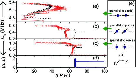
Fig. 1: (Color online) Natural vibration frequencies $\Omega_{0i}$ versus the inverse participation ratio, for the 1D lattice with $N=100$. Panel (a), (b), and (c) correspond respectively to $\mathord{\buildrel\lower 3.0pt\hbox{$\scriptscriptstyle\rightharpoonup$}\over{k}}$-branch, $(\mathord{\buildrel\lower 3.0pt\hbox{$\scriptscriptstyle\rightharpoonup$}\over{k}}\times\mathord{\buildrel\lower 3.0pt\hbox{$\scriptscriptstyle\rightharpoonup$}\over{E}})$-branch, and $\mathord{\buildrel\lower 3.0pt\hbox{$\scriptscriptstyle\rightharpoonup$}\over{E}}$-branch. The open circles are obtained by the rigorous MS-MST formalism and the dotted line is that of the P.E. model (4). Panel (d) shows the $I.P.R.$ for the “ball and spring” model. Panel (e) shows schematically the direction of the particles’ displacements for the three branches.

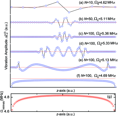
Fig. 2: (Color online) The profiles of a few selected VEMs in the $\mathord{\buildrel\lower 3.0pt\hbox{$\scriptscriptstyle\rightharpoonup$}\over{k}}$-branch. Dashed lines show the equilibrium positions. Each circle represents one particle. Panel (a)-(c): the highest frequency mode for a lattice containing (a): $N=10$ particles, (b): $N=50$, and (c) $N=100$. Panel (c)-(f): the VEMs for $N=100$, with (c) showing the highest frequency mode, and (d)-(e) correspond to two intermediate frequencies, and (f) shows the lowest frequency mode. Note that the interparticle separation and the size of the particles are not drawn to scale. Panel (g) shows $\Omega_{\mbox{intrinsic}}$ with $N=100$, see (8).

References

• [1] A. Ashkin, Phys. Rev. Lett. 24, 156 (1970).
• [2] See e.g. D.G. Grier, Nature 424, 810 (2003).
• [3] M.M. Burns, J.M. Fournier, and J.A. Golovchenko, Science 249, 749 (1990).
• [4] J. Ng, Z.F. Lin, C.T. Chan, and P. Sheng, Phys. Rev. B 72, 085130 (2005); ibid, Opt. Lett. 30, 1956 (2005).
• [5] P.C. Chaumet and M. Nieto-Vesperinas, Phys. Rev. B 64, 035422 (2001).
• [6] D.K. Campbell, S. Flach, and Y.S. Kivshar, Physics Today 57, No. 1, 43 (2004).
• [7] S.A. Tatarkova, A.E. Carruthers, and K. Dholakia, Phys. Rev. Lett. 89, 283901 (2002).
• [8] W. Singer, M. Frick, S. Bernet, and M. Ritsch-Marte, J. Opt. Soc. Am. B 20, 1568 (2003).
• [9] A.T. Black, Hilton, W. Chan, and V. Vuletic, Phys. Rev. Lett. 91, 203001 (2003).
• [10] V. Garces-Chavez and K. Dholakia, Appl. Phys. Lett. 86, 031106 (2005).
• [11] C.D. Mellor and C.D. Bain, ChemPhysChem 7, 329 (2006).
• [12] The stable configurations calculated by the MS-MST formalism deviate from (2) by less than 0.003$\lambda$.
• [13] This is so because, on every sphere, the path difference between the incident field and the scattered field from the other spheres, are roughly an integer multiple of 2$\pi$, which enhances the stability.
• [14] A. Chowdhury and B. Ackerson, Phys. Rev. Lett. 55, 833 (1985).
• [15] N.E. Cusack, The Physics of Structurally Disordered Matter: An Introduction (A. Hilger, Philadelphia, 1987), p. 239.
• [16] The finite coherent length of real laser will effectively set an upper limit on N. In the hypocritical case where $N\to\infty$, the modes for (6)-(7) become extended modes, whereas (5) diverges.
• [17] M.I. Antonoyiannakis and J.B. Pendry, Phys. Rev. B 60, 613 (1997).