Spin cloud induced around an elastic scatterer by the intrinsic spin-Hall effect

Abstract

Similar to the Landauer electric dipole created around an impurity by the electric current, a spin polarized cloud of electrons can be induced by the intrinsic spin-Hall effect near a spin independent elastic scatterer. It is shown that in the ballistic range around the impurity, such a cloud appears in the case of Rashba spin-orbit interaction, even though the bulk spin-Hall current is absent.

The spin-Hall effect attracts much interest because it provides a method for manipulating electron spins by electric gates, incorporating thus spin transport into conventional semiconductor electronics. As it has been initially predicted, the electric field $\mathbf{E}$ induces the spin flux of electrons or holes flowing in the direction perpendicular to $\mathbf{E}$. This spin flux can be due either to the intrinsic spin-orbit interaction (SOI) inherent to a crystalline solid Murakami , or to spin dependent scattering from impurities Hirsch . Intrinsic spin-Hall effect corresponding to the former situation has been observed in p-doped 2D semiconductor quantum wells Wunderlich , while the extrinsic effect related to the latter scenario has been detected in n-doped 3D semiconductor films Awschalom2 .

Most of the theoretical studies on the spin-Hall effect (SHE) has been focused on calculation of the spin current (for a review see Engel ). On the other hand, since the spin current carries the spin polarization, one would expect a buildup of the spin density near the sample boundaries. Such a spin accumulation near interfaces of various nature was calculated in a number of works Accumulation ; Accumulation2 ; ballistic . This accumulated polarization is a first evidence of SHE that has been observed experimentally in Ref. Wunderlich ; Awschalom2 . In fact, measuring spin polarization is thus far the only practical way to detect SHE.

Yet the spin accumulation near interfaces is not the only signature of SHE. To draw an analogy with the charge transport, one can expect that similar to Landauer charge dipoles created by the DC electric current around impurities Landauer , nonequilibrium spin dipoles must be formed subsequent to the spin-Hall current. One may expect that the spin cloud will appear around a spin-orbit scatterer in case of extrinsic SHE, as well as around a spin-independent scatterer, in case of the intrinsic effect. We will consider the latter possibility for a 2D electron gas with Rashba interaction. The polarization in the direction perpendicular to 2DEG will be calculated in the ballistic range around an impurity represented by an isotropic spin independent scattering potential. Besides conventional semiconductor quantum wells this analysis can be applied to metal adsorbate systems with strong Rashba type spin splitting of surface states metalRashba . In this case the spin cloud can be measured by STM with a magnetic tip.

The Landauer electric dipole has been calculated Chu ; Zwerger basing on the asymptotic expansion of the electron waves elastically scattered from an isolated impurity. Subsequent averaging of the corresponding spatial probability weighted by the Boltzmann distribution function of incident wavevectors produces the dipole distribution. The spin cloud could be obtained in a similar way. Instead, we choose a Green function method combined with the linear response theory. Within this method the spin density is given by the standard Kubo formula where the scattering potential of a target impurity, at a fixed position $\mathbf{r}_{i}$, is included into the Green functions, up to the second perturbation order. Other impurities are assumed to be randomly distributed over a 2D plane, so that the calculated spin density is averaged over their positions.

We assume that a uniform external electric field is applied to 2DEG. The field is represented by the vector potential $\mathbf{A}$, $\mathbf{E}=i\omega\mathbf{A}/c$, with $\omega\rightarrow$ 0 in the DC regime. The corresponding interaction Hamiltonian is $e\mathbf{A\cdot v}/c$, where the velocity $\mathrm{v}^{j}$, $j=x,y$, includes the spin-orbit correction $\partial(\mathbf{h}_{\mathbf{k}}\cdot\bm{\sigma})/\partial k^{j}$. The spin-orbit field $\mathbf{h}_{\mathbf{k}}$ is a function of the two-dimensional wave-vector $\mathbf{k}$. In its turn, the spin-orbit interaction is written in the form

$$H_{so}=\mathbf{h}_{\mathbf{k}}\cdot\bm{\sigma}\,,$$ (1)

where $\bm{\sigma}$$\equiv$$(\sigma^{x},\sigma^{y},\sigma^{z})$ is the Pauli matrix vector. We assume that the target impurity, located at $\mathbf{r}_{i}$, has a scattering potential $U(\mathbf{r}-\mathbf{r}_{i})$. In 2D geometry the corresponding Born amplitude is given by

$$f(\mathbf{k},\mathbf{k^{\prime}})=-\frac{m^{*}}{\sqrt{2\pi k_{F}}}\int dr^{2}U(\mathbf{r})e^{i(\mathbf{k}-\mathbf{k^{\prime}})\mathbf{r}}\,,$$ (2)

where $\hbar=1$ and $\varphi$ is the angle between $\mathbf{k}$ and $\mathbf{k^{\prime}}$. Both the scattered and the incident wavevectors are taken at the Fermi circle with the radius $k_{F}$. Other impurities, which not necessarily are of the same nature as the target impurity, are randomly distributed within a sample. They create the random potential $V_{sc}(\mathbf{r})$ which is assumed to be delta correlated, so that the pair correlator $\langle V_{sc}(\mathbf{r})V_{sc}(\mathbf{r}^{\prime})\rangle=\Gamma\delta(\mathbf{r}-\mathbf{r}^{\prime})/\pi N_{F}$, where $N_{F}$ is the electron density of states at the Fermi energy, and $\Gamma=1/2\tau$ is expressed via the mean elastic scattering time $\tau$. Assuming that the semiclassical approximation $E_{F}\tau\gg 1$ is valid, one can apply the standard perturbation theory agd ; alt when calculating the configurational averages of Green functions and their products. In the leading order of $(E_{F}\tau)^{-1}$ and up to the second order in $U(\mathbf{r}-\mathbf{r}_{i})$, the average retarded Green function in the momentum representation is given by

$$G^{r}_{\mathbf{k}\mathbf{k^{\prime}}}(\omega)=\delta_{\mathbf{k}\mathbf{k^{\prime}}}G^{r(0)}_{\mathbf{k}}(\omega)+G^{r(1)}_{\mathbf{k}\mathbf{k^{\prime}}}(\omega)+G^{r(2)}_{\mathbf{k}\mathbf{k^{\prime}}}(\omega)\,,$$ (3)

with the unperturbed function given by the 2$\times$2 matrix

$$G^{r(0)}_{\mathbf{k}}(\omega)=(\omega-E_{\mathbf{k}}-\bm{h}_{\mathbf{k}}\cdot\bm{\sigma}+i\Gamma)^{-1}\,,$$ (4)

where $E_{\mathbf{k}}$=$k^{2}/(2m^{*})$. Other functions in (3) are

$$G^{r(1)}_{\mathbf{k}\mathbf{k^{\prime}}}(\omega) = G^{r(0)}_{\mathbf{k}}(\omega)U_{\mathbf{k}\mathbf{k^{\prime}}}G^{r(0)}_{\mathbf{k^{\prime}}}(\omega)$$ (5)

$$G^{r(2)}_{\mathbf{k}\mathbf{k^{\prime}}}(\omega) = G^{r(0)}_{\mathbf{k}}(\omega)\sum_{\mathbf{k^{\prime\prime}}}U_{\mathbf{k}\mathbf{k^{\prime\prime}}}G^{r(0)}_{\mathbf{k^{\prime\prime}}}(\omega)U_{\mathbf{k^{\prime\prime}}\mathbf{k^{\prime}}}G^{r(0)}_{\mathbf{k^{\prime}}}(\omega)\,.$$

The matrix elements $U_{\mathbf{k^{\prime}}\mathbf{k}}=-\sqrt{2\pi k_{F}}f(\mathbf{k},\mathbf{k^{\prime}})\exp[i(\mathbf{k}-\mathbf{k^{\prime}})\mathbf{r}_{i}]/m^{*}$. Expressions similar to Eqs.(3-5) can be obtained for the advanced functions $G^{a}_{\mathbf{k^{\prime}}\mathbf{k}}(\omega)=G^{r}_{\mathbf{k^{\prime}}\mathbf{k}}(\omega)^{{\dagger}}$. The sum over $\mathbf{k^{\prime\prime}}$ in the second Eq. (5) can be directly calculated. First, we decompose $G^{r(0)}_{\mathbf{k^{\prime\prime}}}$ into a spin independent scalar part and a spin dependent part which is proportional to $\mathbf{h}_{\mathbf{k^{\prime\prime}}}\cdot\bm{\sigma}$. Due to the time inversion symmetry $\mathbf{h}_{\mathbf{k^{\prime\prime}}}=-\mathbf{h}_{-\mathbf{k^{\prime\prime}}}$ the sum over $\mathbf{k^{\prime\prime}}$ on the spin dependent part is zero for an isotropic scattering amplitude. For anisotropic amplitude, however, this sum is not identically 0. Nevertheless, the sum on the spin dependent part can be ignored either way in the following calculations, because it is proportional to the small parameter $h_{k_{F}}/E_{F}\ll 1$. Further, it is easily seen that only $\mathrm{Im}[G^{r(0)}_{\mathbf{k^{\prime\prime}}}]$ is important in this $\mathbf{k^{\prime\prime}}$ sum because the real part gives rise to a term that simply adds to $U_{\mathbf{k}\mathbf{k^{\prime}}}$ in the first line of Eq. (5), thus effectively renormalizing the Born scattering amplitude. The imaginary part can not be absorbed in such a way because it has opposite signs for the advanced and retarded Green functions. Taking into account that $\omega\simeq E_{F}$ and assuming that $h_{k_{F}}\ll E_{F}$ we thus get

$$\sum_{\mathbf{k^{\prime\prime}}}U_{\mathbf{k}\mathbf{k^{\prime\prime}}}G^{r(0)}_{\mathbf{k^{\prime\prime}}}(\omega)U_{\mathbf{k^{\prime\prime}}\mathbf{k^{\prime}}}=-i\pi N_{F}S(\mathbf{k},\mathbf{k^{\prime}})e^{i(\mathbf{k^{\prime}}-\mathbf{k})\mathbf{r}_{i}}\,$$

$$S(\mathbf{k},\mathbf{k^{\prime}})=\frac{k_{F}}{m^{*2}}\int d\varphi^{\prime\prime}f(\mathbf{k^{\prime\prime}},\mathbf{k})f(\mathbf{k^{\prime}},\mathbf{k^{\prime\prime}})\,,$$ (6)

where $\phi^{\prime\prime}$ is the angle of the vector $\mathbf{k^{\prime\prime}}$, with $|\mathbf{k^{\prime\prime}}|=k_{F}$. At $\mathbf{k}=\mathbf{k^{\prime}}$ the integral in (Spin cloud induced around an elastic scatterer by the intrinsic spin-Hall effect) is equal to the scattering cross-section.

Within the semiclassical theory we follow the well known method agd ; alt to calculate the configurational average of the Green functions product that enters into the Kubo’s linear response equation. Because of scattering on a target impurity this product contains more than a pair of Green functions. As our leading approximation we take into account the so called ladder perturbation series describing particle and spin diffusion processes. When averaging the Green function product, within this approximation, only pairs of retarded and advanced functions carrying close enough momenta should be chosen to become elements of the ladder series. This considerably simplifies calculations. Some of the representative diagrams are shown at Fig. 1, where $\mathbf{v}$ denotes the velocity operator

$$\mathrm{v}^{j}=\frac{k^{j}}{m^{*}}+\frac{\partial\mathbf{h}_{\mathbf{k}}\cdot\bm{\sigma}}{\partial k^{j}}\,.$$ (7)

The diffusion ladder renormalizes only the vertex associated with the electric field, while such a ladder, as we just explained, does not appear at the vertex attributed to the induced spin density. It is because in the ballistic range around the impurity, the momentum transfer $|\mathbf{p}-\mathbf{k}|\gg 1/(v_{F}\tau)$, and thus the diffusion is not important. Finally, the density of spins oriented in $z$ direction can be written as

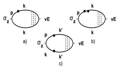
Figure 1: Diagram for the spin density. Scattering of electrons by a target impurity is shown by the solid circles. Dashed lines denote the ladder series of particle scattering by the random potential. $\mathbf{p},\mathbf{k},\mathbf{k^{\prime}}$ are electron momenta.

$$\sigma_{z}(\mathbf{r}) = \sum_{\mathbf{k},\mathbf{k}^{\prime},\mathbf{p}}e^{i(\mathbf{p}-\mathbf{k})\mathbf{r}}\int\frac{d\omega}{2\pi}\frac{dn_{F}(\omega)}{d\omega}\times$$ (8)

$$Tr[G^{a}_{\mathbf{k}^{\prime}\mathbf{k}}(\omega)\sigma_{z}G^{r}_{\mathbf{p}\mathbf{k}^{\prime}}(\omega)\mathcal{T}(\omega,\mathbf{k^{\prime}})]\,,$$

where the trace runs through the spin variables and $n_{F}(\omega)$ is the Fermi distribution function. The functions $G^{r/a}_{\mathbf{k}^{\prime}\mathbf{k}}$ are given by Eq. (3). In (8), only terms up to the second order in $U_{\mathbf{k^{\prime}}\mathbf{k}}$ should be taken into account. Hence the highest order corrections are those shown at Fig.1, b) and c). At low temperatures only $\omega$ in close vicinity around $E_{F}$ contributes to the integral in (8). Therefore, below we set $\omega=E_{F}$.

It is important that the vertex $\mathcal{T}(\omega,\mathbf{k})$ in Eq.(8) is the same that enters into the spin-Hall conductance. On the other hand, as was shown in many publications Inoue , for linear in $\mathbf{k}$ SOI and $h_{\mathbf{k}}\ll E_{F}$, a contribution to $\mathcal{T}(\omega,\mathbf{k})$ from the spin dependent part of the velocity (7) cancels with its spin independent part, while such a cancellation does not take place in case of nonlinear SOI MalshDress . As a result of such cancellation, in a linear case $\mathcal{T}(\omega,\mathbf{k})$ is reduced to the simple expression

$$\mathcal{T}(\omega,\mathbf{k})=\frac{e}{m^{*}}\mathbf{k}\mathbf{E}\,.$$ (9)

Let us consider the spin density (8) in the presence of the Rashba spin-orbit field $h_{x}=\alpha k_{y},h_{y}=-\alpha k_{x}$. In the zeroth order in $U_{\mathbf{k}\mathbf{k^{\prime}}}$ the Green functions in (8) are given by the first term in (3). In this approximation and with $\mathcal{T}$ given by (9) one can easily see that $\sigma_{z}(\mathbf{r})=0$. On the other hand, the inplane spin polarization directed perpendicular to $\mathbf{E}$ is finite. This polarization is due to the electric orientation effect Edelstein . In the first order with respect to $U_{\mathbf{k}\mathbf{k^{\prime}}}$ the z spin polarization is represented by Fig.1a. Expressing $U_{\mathbf{k}\mathbf{k^{\prime}}}$ via the scattering amplitude, from (3-5) and (8) we obtain

$$\sigma_{z}^{(a)}(\mathbf{r}) = -e\sqrt{\frac{k_{F}}{2\pi}}\sum_{\mathbf{k},\mathbf{p}}\frac{\mathbf{k}\mathbf{E}}{m^{*2}}Tr[G^{r0}_{\mathbf{k}}(E_{F})G^{a0}_{\mathbf{k}}(E_{F})\times$$ (10)

$$\left(\sigma_{z}G^{r0}_{\mathbf{p}}(E_{F})f(\mathbf{p},\mathbf{k})e^{i(\mathbf{p}-\mathbf{k})\mathbf{R}}+h.c.\right)]\,,$$

where $\mathbf{R}=\mathbf{r}-\mathbf{r}_{i}$. At $kR,pR\gg 1$ the 2D angular integration in (10) can be performed by expansions around the saddle-points $(\mathbf{p}\mathbf{R}/pR)=\pm 1$ and $(\mathbf{k}\mathbf{R}/kR)=\pm 1$, that result in the asymptotic expansion of $\sigma_{z}(\mathbf{r})$ at a large distance from the impurity. The remaining integrals over $p$ and $k$ are dominated by contributions from the poles of Green functions (4). These poles are located at $k,p=\pm k_{F}\pm L_{so}^{-1}\pm il^{-1}$, where $L_{so}=\hbar/m^{*}\alpha\gg k_{F}^{-1}$ is the characteristic spin-orbit length and $l$ is the mean free path. In the ballistic range $R\lesssim l$ one may substitute the imaginary part $il^{-1}$ of the poles by $i\delta$ with $\delta\rightarrow 0$. Depending on combination of  $\pm$  signs of the poles, the scattering amplitude entering into (10) will coincide either with the forward scattering amplitude $f(0)=f(k_{F}\mathbf{\hat{R}},k_{F}\mathbf{\hat{R}})$, or with the backscattering amplitude $f(\pi)=f(k_{F}\mathbf{\hat{R}},-k_{F}\mathbf{\hat{R}})$, where $\mathbf{\hat{R}}=\mathbf{R}/R$ is the unit vector directed to the observation point. Finally, we obtain from (10) and (4)

$$\sigma_{z}^{(a)}(\mathbf{r}) = \frac{m^{*}}{R}\sqrt{\frac{2}{\pi^{3}k_{F}}}v^{j}_{d}\left(\frac{\partial\mathbf{n}_{R}}{\partial R^{j}}\times\mathbf{n}_{R}\right)\times$$ (11)

$$\mathrm{Re}[f(\pi)e^{2ik_{F}R}]\sin^{2}\left(\frac{R}{L_{so}}\right)\,,$$

where $\mathbf{v}_{d}=e\tau\mathbf{E}/m^{*}$ is the drift velocity. The unit vector $\mathbf{n}_{R}=\mathbf{h}_{k_{F}\mathbf{\hat{R}}}/|h_{k_{F}\mathbf{\hat{R}}}|$. For Rashba interaction it is $n_{R}^{x}=\hat{R}^{y},\,n_{R}^{y}=-\hat{R}^{x}$.

In a similar way and with the use of Eq.(Spin cloud induced around an elastic scatterer by the intrinsic spin-Hall effect) one can calculate the second order contribution to the spin density, that is represented in Fig. 1b) and c). Assuming the electric field to be applied in the $x$-direction, we get the final result, which is as a sum of all diagrams in Fig. 1a)-c),

$$\sigma_{z}(\mathbf{r}) = -\frac{m^{*}v_{d}\sigma_{t}}{2\pi^{2}RL_{so}}\sin\left(\frac{2R}{L_{so}}\right)\sin\theta+$$ (12)

$$\frac{m^{*}v_{d}}{2\pi^{2}R^{2}}\sin^{2}\left(\frac{R}{L_{so}}\right)\sin^{3}\theta\times$$

$$\left(\sigma_{tot}+\sqrt{\frac{8\pi}{k_{F}}}\mathrm{Re}[f(\pi)e^{2ik_{F}R}]\right)\,,$$

where $\sigma_{tot}$ and $\sigma_{t}$ are the total and transport scattering cross sections, respectively, and $\theta$ is the angle between the vector $\mathbf{R}$ and the x-axis. In order to check our method we applied it to the calculation of the charge dipole, whence $\sigma_{z}$ is substituted by 1 in Eq. (8). Ignoring SOI we obtained the same result as in Ref.Zwerger .

The explicit shape of the spin cloud is clearly seen from Eq. (12). It consists of a dipole, oriented perpendicular to the electric field, and a tripole. Similar to the Landauer charge dipole distribution Zwerger , the spin density contains both slowly varying and fast Friedel oscillation components. Important distinctions, however, are found in the asymptotic behaviors. First, unlike the charge density, whose slow asymptotic term is represented by monotonous $R^{-1}$ dependence, the spin density oscillates with a period determined by the spin-orbit precession length $\pi L_{so}$. Second, at smaller distances $R\lesssim L_{so}$, the polarization decreases as $R^{-2}$. It should be noted that this asymptotic form can not be obtained by the method based on the conventional leading order asymptotic expansion of the wave function, as it has been done in Zwerger for the Landauer dipole. It is because in 2D geometry the corresponding scattered amplitude decreases as $1/\sqrt{R}$. Accordingly, the probability density, which can be either the charge or the spin density, will be proportional to $1/R$, not $1/R^{2}$.

When talking about asymptotic expression (12), one should not forget that it is valid only within the ballistic range $R\lesssim l$. At larger distances the ballistic part of the spin density decays as $exp(-R/l)$. On the other hand, outside the ballistic range the spin diffusion becomes important. Spin diffuses during the D’yakonov-Perel’ dp spin relaxation time, up to the distance $\sim L_{so}$. Hence, the spin diffusion must be taken into account at $R\gg l$, providing that the spin-orbit coupling is not too strong, so that $L_{so}\gg l$. In order to calculate the spin density in the diffusive range, the ladder diagrams renormalizing the left hand vertex in Fig. 1 should be taken into account. An evident result to be expected in this case is that the diffusion spin cloud with the size $\gg l$ will appear in addition to Eq.(12). Due to the spin relaxation, however, the spin density will decay exponentially at $R\gg L_{so}$. This behavior is in sharp contrast to the power law decreasing of the charge density Chu . In the latter case, the long-range $R^{-1}$ charge-density tails of many impurities result in the macroscopic electric field which can be related to the electric potential difference at the sample boundaries. This was the main idea by Landauer - to associate impurities with resistors which give rise to an overall potential drop at a given current. Similarly, one would try to formulate the spin-Hall effect in terms of the spin-Hall resistance and spin dependent chemical potential $\chi(\mathbf{r})$, defined as $N_{F}\chi(\mathbf{r})=\sum_{i}\sigma_{z}(\mathbf{r}-\mathbf{r}_{i})$. In such a way an influence of disorder on SHE can be considered from the microscopic point of view starting from individual impurities. For example, similar approach has been employed in a semiclassical analysis of the side jump contribution to the anomalous Hall effect Sinitsyn . Returning to the spin potential $\chi(\mathbf{r})$, one can notice that due to exponential decay in space of the spin cloud, the well converging sum over impurities will produce, on average, a vanishing spin-Hall chemical potential everywhere, except for the $R\sim L_{so}$ range near the sample boundary. No such spin accumulation, on the other hand, has been found near hard wall flanks of a 2D diffusive strip of 2DEG with Rashba SOI Accumulation2 . At the same time the finite accumulation was calculated in Accumulation for other boundary conditions. Probably, this means that the spin density outside the ballistic range around an elastic scatterer is finite, but the combined spin density produced by many impurities will depend on the boundary conditions for spin diffusion.

In conclusion, for a 2DEG with Rashba spin-orbit interaction we calculated the nonequilibrium spin polarization induced by the intrinsic spin-Hall effect in the ballistic range around a spin independent scatterer. The angular spatial distribution of the spin density is represented by a tripole and a dipole oriented perpendicular to the electric field. As a function of the distance from the scatterer, the polarization shows the power law decay with oscillations, some terms oscillating relatively slowly, with the period $\pi L_{so}$, while other terms varying fast, with a period of Friedel oscillations. Noteworthy, that although the z-polarized spin-Hall current is zero in case of Rashba SOI, we found out that the z-component of the spin density is not zero in the ballistic range. This agrees with finite spin accumulation near flanks of a ballistic strip ballistic .

This work was supported by the Taiwan National Science Council NSC94-2811-M-009-010 and RFBR Grant No 060216699. A.G.M. acknowledges the hospitality of Taiwan National Center for Theoretical Sciences.

References

- (1) S. Murakami, N. Nagaosa, and S.-C. Zhang, Science 301, 1348 (2003); J. Sinova et. al., Phys. Rev. Lett. 92, 126603 (2004); D. Culcer et. al., Phys. Rev. Lett. 93, 046602 (2004).
- (2) M. I. Dyakonov, V. I. Perel, Phys. Lett. A 35, 459 (1971); J. E. Hirsch, Phys. Rev. Lett 83, 1834 (1999).
- (3) Y. K. Kato, et. al., Science 306, 1910 (2004)
- (4) J. Wunderlich et. al., Phys. Rev. Lett. 94, 047204 (2005)
- (5) H. -A. Engel, E. I. Rashba, and B. I. Halperin, cond-mat/0603306.
- (6) V. M. Galitski et. al., cond-mat/0601677; G. Usaj and C. Balsiero, cond-mat/0405065; İ. Adagideli and G.E.W. Bauer, Phys. Rev. Lett. 95, 256602 (2005);
- (7) A. G. Mal’shukov et. al., Phys. Rev. Lett. 95, 146601 (2005); R. Raimondi et. al., cond-mat/0601525;
- (8) B. K. Nikolić et. al., Phys. Rev. Lett. 95, 046601 (2005); Q. Wang et. al., cond-mat/0505576.
- (9) R. Landauer, IBM Journ. Res. Development, 1, 223 (1957); R. Landauer, Philos. Mag. 21,863 (1970).
- (10) R. S. Sorbello and C.S. Chu, IBM J. Res. Develop. 32, 58 (1988); C.S. Chu and R. S. Sorbello, Phys. Rev. B 38, 7260 (1988)
- (11) W. Zwerger, L. Bönig, and K. Schonhammer, Phys. Rev. B 43, 6434 (1991)
- (12) C. R. Ast et. al. cond-mat/0509509 unpublished
- (13) A.A. Abrikosov, L.P. Gor’kov, and I.E. Dzyaloshinskii, Methods of Quantum Field Theory in Statistical Physics, (Dover, New York, 1975)
- (14) B. L. Altshuler and A. G. Aronov, in Electron-Electron Interactions in Disordered Systems, edited by A. L. Efros and M. Pollak (North-Holland, Amsterdam, 1985).
- (15) J. I. Inoue, G. E. W. Bauer, and L.W. Molenkamp, Phys. Rev. B 70, 041303 (2004); E. G. Mishchenko, A. V. Shytov, and B. I. Halperin, Phys. Rev. Lett. 93, 226602 (2004); E. I. Rashba, Phys. Rev. B 70, 201309(R) (2004); R. Raimondi and P. Schwab, Phys. Rev. B 71, 033311 (2005).
- (16) A. G. Mal’shukov and K. A. Chao, Phys. Rev. B 71, 121308(R) (2005)
- (17) V.M. Edelstein, Solid State Commun., 73, 233 (1990); J. I. Inoue, G. E. W. Bauer, and L.W. Molenkamp, Phys. Rev. B 67, 033104 (2003)
- (18) M. I. D’yakonov and V. I. Perel’, Sov. Phys. JETP 33, 1053 (1971) [Zh. Eksp. Teor. Fiz. 60, 1954 (1971)].
- (19) N. A. Sinitsyn, Q. Niu, and A. H. McDonald, Phys. Rev. B 73, 075318 (2006).