Communication models with distributed transmission rates and buffer sizes

Abstract

The paper is concerned with the interplay between network structure and traffic dynamics in a communications network, from the viewpoint of end-to-end performance of packet transfer. We use a model of network generation that allows the transition from random to scale-free networks. Specifically, we are able to consider three different topological types of networks: (a) random; (b) scale-free with $\gamma=3$; (c) scale-free with $\gamma=2$. We also use an LRD traffic generator in order to reproduce the fractal behavior that is observed in real world data communication. The issue is addressed of how the traffic behavior on the network is influenced by the variable factors of the transmission rates and queue length restrictions at the network vertices. We show that these factors can induce drastic changes in the throughput and delivery time of network performance and are able to counter-balance some undesirable effects due to the topology.

I Introduction

We consider the class of networks generated by the model introduced in [1]. This model is particularly interesting since it allows a parametrized transition between random (homogenous) and scale-free (heterogenous) graphs. In particular, scale-free graphs are characterized by the presence of few very high degree vertices, called hubs, which are responsible for a drastic reduction of the average distance between network nodes.

In [2], we have already studied the effects of such a transition on the network communication performance. The main result shows that, somewhat surprisingly, the structure of scale-free graphs, which are ubiquitous in nature, does not lead to any benefit but rather a worsening in terms of the end-to-end performance. In particular, the characteristic parameters known as throughput and delivery time were considerably affected by the congestion at the network hubs. This is counter-intuitive when one considers that the shortening of the distances in the network might result in a reduction of the delivery time and thus an increase of the throughput.

This interesting phenomenon is analogous to the paradox of heterogeneity [3], which has been observed in the context of synchronizability of scale-free networks. Indeed, it is unrealistic to assume that resources such as bandwidth are uniformly distributed among the network nodes in strongly heterogenous networks. Instead, it is very likely that hubs, which are characterized by a high number of incoming and outgoing links, are found to play a fundamental role in communication over the network. They are typically characterized by having higher server strength transmission rates and larger buffers than more peripheral nodes. For that reason we consider here the following variation to the study presented in [2]:

• The transmission rate $r$ is assumed to scale with the degree at each vertex $i$, $k(i)$, as: $r(i)=c_{1}k(i)^{\alpha}$ (note that in the particular case where $\alpha=0$, we recover the original case, with all the nodes having the same transmission rates);

• the maximum queue length (i.e., the buffer size) is no longer assumed infinite but is taken to scale with the degree at each vertex $i$, $k(i)$, as: $q(i)=c_{2}k(i)^{\beta}$.

We use the power laws above not necessarily for accurate simulation of the nature of distributed transmission rates and buffer sizes, but for their qualitative properties which emphasizes the importance of these hubs. In what follows, we analyze separately, by means of numerical simulations, the effects of varying $\alpha$ and $\beta$ on the network communication performance. As a representative case, we assume $c_{1}=1$ and $c_{2}=50$. Similar behaviour was observed for other values of $c_{1}$ and $c_{2}$.

Then we compare the behaviors of networks characterized by different topological features. More precisely, networks will be considered with different degree distributions; the degree $k$ at a given node being the number of incident links at the node. Particular emphasis will be given to scale-free topologies in which the degree distribution is observed to follow a power law, i.e. $P(k)\sim k^{-\gamma}$ [4, 5, 6, 7].

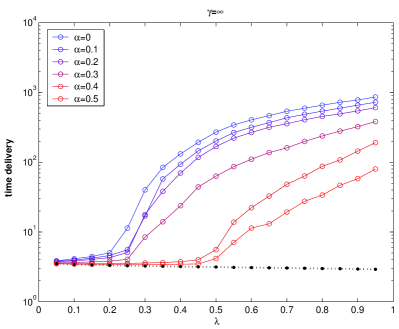
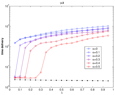
Figure 1: Delivery time versus the generation rate, $\lambda$. The network is a (a) random graph ($\gamma=\infty$), (b) scale-free graph ($\gamma=3$) with number of nodes $N=512$ and number of edges $M=2N$. We show the effects of varying the transmission rates $r(i)$ at node $i$, according to the law $r(i)=k(i)^{\alpha}$, for $\alpha$ ranging between $0$ and $0.5$ (blue to red). The black dotted line represents the free regime at $\alpha=1$.

II Network Topology

We consider networks with assigned topologies overlayed by a packet traffic communication dynamic. We try to characterize the way in which the underlying topology can affect the network behavior and performance by varying the values of the scale-free degree distribution exponent $\gamma$.

There are many classical models for the production of network topologies, but they lack the ingredient of specific degree characteristics. The famous $Erd\ddot{o}s-Ren\acute{y}i$ [8] random network algorithm leads to networks with Poissonian degree distribution, which are characterized by an exponential cut-off for high degrees. This is based on a very simple procedure, namely a network with $N$ vertices and $M$ edges is built as follows: we select with uniform probability two of the $N$ possible vertices and link them unless they are either already connected or self-links are generated. We repeat this iteration $M$ times.

In order to cause the transition from random to scale-free network we use the static model introduced in [1]. Vertices are indexed by an integer $i$, for $(i=1....,N)$, and assigned a weight or fitness $p_{i}=i^{-\eta}$ where $\eta$ is a parameter between 0 and 1. Two different vertices are selected with probabilities equal to the normalized weights, $p_{i}/\sum_{k}{p_{k}}$ and $p_{j}/\sum_{k}{p_{k}}$, and an edge is added between them unless one exists already. This process is repeated until $M$ edges are made in the system leading to the mean degree $\langle k\rangle=2M/N$. This results in the expected degree at vertex $i$ scaling as $k_{i}\sim(\frac{N}{i})^{\eta}$ [1]. We then have the degree distribution, i.e. the probability of a vertex being of degree $k$, given by $P(k)\sim k^{-\gamma}$ with $\gamma=1+\frac{1}{\eta}$. Thus, by varying $\eta$, we can obtain the exponent $\gamma$ in the range, $2<\gamma<\infty$. Moreover the ER graph is generated by taking $\eta=0$.

It is worth noting that the static model described here can be considered as an extension of the standard ER model for generating random scale-free networks, i.e. networks with prescribed degree distribution, but completely random with respect to all the other features.

III Model of Network Data Traffic

We use the family of Erramilli interval maps as the generator for each LRD traffic source within the network [9]. The maps are given by $f=f_{(m_{1},m_{2},d)}:I\rightarrow I$, $I=[0,1]$, where:

$$f(x)=\begin{cases}x+(1-d)\left({x/d}\right)^{m_{1}},&x\in[0,d],\cr x-d\left((1-x)/(1-d)\right)^{m_{2}},&x\in(d,1],\end{cases}$$ (1)

where $d\in(0,1)$. The map $f$ is iterated to produce an orbit, or sequence, of real numbers $x_{n}\in[0,1]$ which is then converted into a binary Off-On sequence where the $n$-th value is ‘Off’ if $x_{n}\in[0,d]$, and ‘On’ if $x_{n}\in(d,1]$. If the orbit is in the ‘On’ state, each iteration of the map represents a packet generated. The parameters $m_{1},m_{2}\in[3/2,2]$ induce map intermittency. When $m_{1}=m_{2}=1.5$ we have short range dependent binary output and this becomes fully long range dependent binary output for $m={\rm Max}\{m_{1},m_{2}\}=2.0$. The indicator of long-range dependence is given by the Hurst parameter $H=(3m-4)/(2m-2)$.

The network involves two types of nodes: hosts and routers. The first are nodes that can generate and receive messages and the second can only store and forward messages. The density of hosts, say $\rho\in[0,1]$, is the ratio between the number of hosts and the total number of nodes in the network (in this paper we take $\rho=0.16$). Hosts are randomly distributed throughout the network.

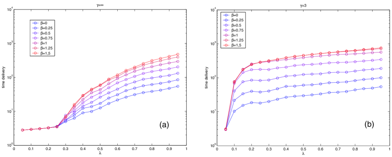
Figure 2: Delivery time versus the generation rate, $\lambda$. The network is a (a) random graph ($\gamma=\infty$), (b) scale-free graph ($\gamma=3$) with number of nodes $N=512$ and number of edges $M=2N$. We show the effects of varying the queue length $q(i)$ at node $i$, according to the law $q(i)=50k(i)^{\beta}$, for $\beta$ ranging between $0$ and $1.5$ (blue to red).

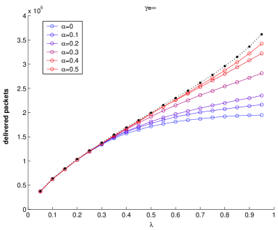
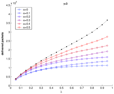
Figure 3: Number of delivered packets versus the generation rate, $\lambda$. The network is a (a) random graph ($\gamma=\infty$), (b) scale-free graph ($\gamma=3$) with number of nodes $N=512$ and number of edges $M=2N$. We show the effects of varying the transmission rates $r(i)$ at node $i$, according to the law $r(i)=k(i)^{\alpha}$, for $\alpha$ ranging between $0$ and $0.5$ (blue to red). The black dotted line represents the free regime at $\alpha=1$.

Packets enter the queue from one side (the end) and leave it from the other one (the head). The head of the queue contains a variable number of packets equal to the transmission rate at the node. The queue at each node $i$, has a finite maximum length, $q(i)$. If the packets arriving at the queue at vertex $i$ result in the number of packets exceeding $q(i)$, then the excess packets are dropped.

A routing algorithm is needed to model the dynamic aspects of the network. Packets are created at hosts and sent through the network one step at a time until they reach their destination host.

The routing algorithm operates as follows:

(1) First, a host creates a packet following a distribution defined by a chaotic map (LRD), as described above. If a packet is generated it is put at the end of the queue for that host. This is repeated for each host in the lattice.

(2) Packets at the head of each queue are picked up and sent to a neighboring node selected according to the following rules. (a) A neighbor closest to the destination node is selected. (b) If more than one neighbor is at the minimum distance from the destination, the link through which the smallest number of packets have been forwarded is selected. (c) If more than one of these links shares the same minimum number of packets forwarded, then a random selection is made.

(3) Packets at the head of each queue, exceeding its maximum capability, are dropped.

This process is repeated for each node in the graph. The whole procedure of packet generation and movement represents one time step of the simulation.

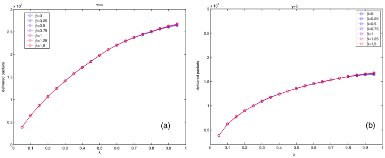
Figure 4: Number of delivered packets versus the generation rate, $\lambda$. The network is a (a) random graph ($\gamma=\infty$), (b) scale-free graph ($\gamma=3$) with number of nodes $N=512$ and number of edges $M=2N$. We show the effects of varying the queue length $q(i)$ at node $i$, according to the law $q(i)=50k(i)^{\beta}$, for $\beta$ ranging between $0$ and $1.5$ (blue to red).

IV Network Performance

Using the network model and traffic generator detailed above, simulations were carried out to analyse various aspects of end-to-end performance for two types of network. Namely, results for random graphs have been paired with those of scale-free graphs with $\gamma=3$. We have calculated the corresponding output for scale-free graphs with $\gamma=2$ and have found that the differences in behaviour with the alternative value $\gamma=3$ are negligible by comparison with the behaviour of the random graph, and so the third set of comparisons is not repeated here.

In Fig. 1 we see that random graphs respond more quickly with smaller delivery times as $\alpha$ increases (from zero). Fig. 2 shows that the communication is much more efficient in terms of delivered packets at high loads (or generation rate) as $\alpha$ increases. Moreover, as shown in Fig. 3 (where the effects of variable transmission rates have been highlighted), scale-free networks behave worse than random graphs for a sufficiently high value of the parameter $\alpha$ (of the order of unity, from our simulations). The number of delivered packets, shown in Fig. 4, instead, is observed to be unaffected by the buffer sizes at the nodes, being mainly determined by the network topology. Finally, in Fig. 5, the number of dropped packets is observed to decrease as the buffer sizes are scaled more sensitively with vertex degree.

V Conclusions

We have analyzed several features of a representative model of communication networks contrasting the network performance when the graph considered is random or scale-free. The results show that there is no obvious benefit for communication networks having scale-free growth patterns across all performance indicators. Nevertheless, the graphs reported here show several critical phenomena with a set of threshold values whose analytical investigation will be the subject of future work.

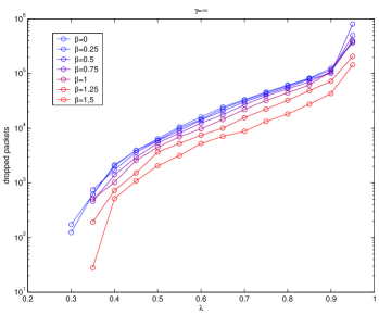
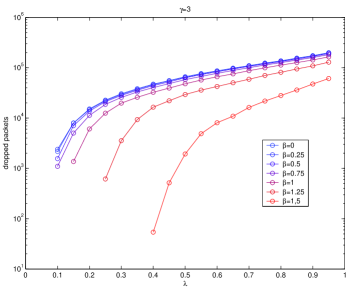
Figure 5: Number of dropped packets versus the generation rate, $\lambda$. The considered network is scale-free with $\gamma=3$ and $\gamma=\infty$, the number of nodes being $N=512$ and number of edges $M=2N$. We show the effects of varying the queue length $q(i)$ at node $i$, according to the law $q(i)=50k(i)^{\beta}$, for $\beta$ ranging between $0$ and $1.5$.

References

- [1] K.-I. Goh, B. Kahng, and D.Kim, “Universal behavior of load distribution in scale-free networks,” Phys.Rev.Lett., vol. 87, no. 27, 2001.
- [2] D.K. Arrowsmith, M. di Bernardo, and F.Sorrentino, “Effects of variation of load distribution on network performance,” Proc. IEEE ISCAS, Kobe, Japan, 2005.
- [3] A.E. Motter, C. Zhou, and J.Kurths, “Network synchronization, diffusion, and the paradox of heterogeneity,” Phys.Rev.E, vol. 71, no. 016116, 2005.
- [4] A.L.Barabasi and R.Albert, “Emergence of scaling in random networks,” Science, vol. 286, pp. 509–512, 1999.
- [5] M.Faloutsos, P.Faloutsos, and C.Faloutsos, “What does internet look like?,” Comput.Commun.Rev., vol. 29, pp. 251–263, 1999.
- [6] L.A.N. Amaral, A. Scala, M.Berth lemy, and H.E.Stanley, “Classes of small-world networks,” Proc.Natl.Acad.Sci.USA, vol. 97, pp. 11149–11152, 2000.
- [7] S.N.Dorogovstev and J.F.F. Mendes, “Evolution of networks,” Adv. Phys, vol. 1079, no. 51, pp. 1079–1187, 2002.
- [8] P. Erdos and A.Renyi, ,” Publ. Math. Inst. Hung. Acad., vol. 5, no. 17, 1960.
- [9] A. Erramilli, R.P. Singh, and P. Pruthi, “Chaotic maps as models of packet traffic,” Proc. Int. Teletraffic Conf., 1994, North–Holland (Elsevier).