Community Detection as an Inference Problem

Abstract

We express community detection as an inference problem of determining the most likely arrangement of communities. We then apply belief propagation and mean-field theory to this problem, and show that this leads to fast, accurate algorithms for community detection.

Community detection is a well-studied problem in networksnr . This is the problem of dividing a network into communities, such that nodes within the same community tend to be connected by links, while those within different communities tend not to be connected by links. This problem has applications in understanding the structure of social and biological networksapplic , while the closely related graph partitioning problem discussed below has applications in parallel processing, to allocate assignments to different processors while minimizing interprocessor communication.

Unfortunately, despite all this interest, there is no formal definition of the problem. Instead, each author tends to define communities as being whatever is found by a particular community detection algorithmcdr2 . In this work, we exploit a standard method of testing communities, the four groups testng , to express community detection as an inference, or maximum likelihood problem. This leads to a derivation of a Potts model similar to those derived previously on phenomenological groundspotts .

To solve this inference problem, we must find the ground state of the Potts model. To do this, we turn to the techniques of belief propagationbelief , also known as sum-product, and mean-field theory. Belief propagation was originally developed to perform decoding in a certain class of error correcting codes, called low-density parity check codesbpb . In this problem, one has a sender and receiver communicating over a noisy channel, and the receiver must determine which of all the possible messages is the most likely. This problem can be mapped onto finding the ground state of a spin system on a particular graphsourlas . The belief propagation algorithm exploits the fact that the graph has a low density of loops to solve this problem, in a manner similar to the famous Bethe-Peierlsbethe solution for the thermodynamics of a spin system on a Bethe lattice.

We will find that the resulting belief propagation algorithm for community detection is highly accurate on the four groups problem, while also performing well on other test networks. We then discuss the scaling of computational time with system size, extensions of this algorithm, and other problems.

Inference Problem— To express community detection as an inference problem we consider the following method, often used to test community detection algorithmsng . We invent a network as follows: we consider $N$ nodes, divided into $q$ different communities with $n_{k}$, $k=1,...,q$ nodes in each community. We consider each pair of nodes in turn. We connect those nodes with probability $p_{in}$ if they lie within the same community and $p_{out}$ if they lie within different communities. We then run the community detection algorithm and see if it correctly assigns nodes to communities. Let $q_{i}$ be the initial assignment of a community to node $i$. The probability that a given graph arises from this procedure is equal to

$$p(\{q_{i}\})=$$ (1)

$$\left(\prod_{k=1}^{q}(1-p_{in})^{n_{k}^{2}/2-n_{k}/2}\right)\left(\prod_{k=1}^{q-1}\prod_{l=k+1}^{q}(1-p_{out})^{n_{k}n_{l}}\right)\times$$

$$\left(\prod_{<ij>}(\frac{p_{in}}{1-p_{in}})^{\delta_{q_{i},q_{j}}}\right)\left(\prod_{<ij>}(\frac{p_{out}}{1-p_{out}})^{1-\delta_{q_{i},q_{j}}}\right)$$

where $\prod_{<ij>}$ denotes a product over pairs of vertices $i,j$ connected by an edge. To verify the correctness of this formula, first consider the case in which there are no edges at all in the graph. Then, the probability is given correctly by the first two products of Eq. (1). Adding edges to the graph changes the probability as given by the second two products in Eq. (1).

We now consider a given graph and formulate the problem as follows: find the most likely community assignment. Following Bayes’ theorem, given a graph, the probability that any given community assignment is the “correct” assignment is proportional to the probability $p(\{q_{i}\})$ multiplied by the a priori probability of having a given $n_{k}$. Throughout this paper we assume the a priori probability of a given $n_{k}$ is constant, and thus the optimal community assignment maximizes the probability in Eq. (1); any non-constant priori probability can be easily incorporated by adding additional terms.

We rewrite Eq. (1) as an exponential:

$$p(\{q_{i}\})=c\exp[\sum_{<ij>}J\delta_{q_{i},q_{j}}]\exp[\sum_{i\neq j}J^{\prime}\delta_{q_{i},q_{j}}/2],$$ (2)

where $\sum_{<ij>}$ denotes a sum over pairs of $i,j$ connected by an edge in the graph, and $c=\exp[\log(1-p_{out})N(N-1)/2]\exp[\sum_{<ij>}\log(p_{out}/(1-p_{out})]$, and with

$$J=\log[(p_{in}(1-p_{out}))/((1-p_{in})p_{out})],$$ (3)

$$J^{\prime}=\log[(1-p_{in})/(1-p_{out})].$$

The factor of $1/2$ in Eq. (2) is to avoid double counting. Eq. (2) presents the probability as a Potts model problem with combined short- and long-range interactions, with coupling constants $J,J^{\prime}$. The problem of community detection is then reduced to finding the ground state of this Potts model. Assuming $p_{in}>p_{out}$, the short-range interactions are ferromagnetic, favoring the assignment of neighboring nodes to the same community, while the long-range interactions are anti-ferromagnetic and prevent one from simply taking all nodes to lie within the same community. The problem of finding the ground state is very closely related to the NP-complete problem of graph partitioning, to break a graph up into partitions, minimizing the number of edges connecting partitions and minimizing the difference in number of nodes between partitions.

Belief Propagation— Having arrived at Eq. (2) we have a very similar problem to that studied in potts . Instead of using Monte Carlo methods to find the ground state, we adopt the method of belief propagation, which we believe to be more efficient for many of the community detection problems that arise. Indeed, for the inference problems which arise many in error correcting codes, belief propagation is the most efficient method.

We begin by taking a mean-field approximation for the long-range interactions, justified for large $N$. We approximate $p(\{q_{i}\})\approx p_{mft}(\{q_{i}\})$, where

$$p_{mft}(\{q_{i}\})\equiv Z^{-1}\exp[\sum_{<ij>}J\delta_{q_{i},q_{j}}]\exp[\sum_{i}h_{i}(q_{i})]$$ (4)

where $Z$ is a normalization, and for $r=1...q$ we define $h_{i}(r)=J^{\prime}N\rho(r)-J^{\prime}p_{i}(r)$ and $\rho(r)=\sum_{i}p_{i}(r)/N$, with

$$p_{i}(r)=\frac{\sum_{\{q_{j}\},q_{i}=r}p_{mft}(\{q_{j}\})}{\sum_{\{q_{j}\}}p_{mft}(\{q_{j}\})},$$ (5)

so that $p_{i}(r)$ is the probability in the mean-field approximation that node $i$ belongs to community $r$. These are a set of self-consistent equations for $p_{i}(q)$.

We will find that solving these equations, at least in the belief propagation approximation below, leads to a spontaneous symmetry breaking: for sufficiently large $J,J^{\prime}$, the probability $p_{i}(q)$ depends on $q$. Of course, given any solution which breaks symmetry, one can arrive at other valid solutions by relabeling the communities. We then make a “nodewise” maximum a posteriori probability (MAP) approximation: for each node $i$, we compute $p_{i}(q)$ and then assign the node $i$ to the community $q$ which maximizes $p_{i}(q)$. This is an approximation: the set of community assignments which maximizes $p(\{q_{i}\})$ may not be given by maximizing the probability for each node separately. However, similar approximations work very well for error correcting codesbpb , and these approximations are justified for large $J,J^{\prime}$.

To compute the $p_{i}(q)$, we apply belief propagation. Suppose the graph forms a tree, with no loops. Then, the problem of solving for $p_{i}(q)$ given $h_{i}(q)$ can be solved: for each pair of nodes $i,j$ connected by an edge, we define $p_{ij}(r)$ to be probability $p_{i}$ for the network modified by removing the edge connecting $i$ to $j$. That is,

$$p_{ij}(r)=\frac{\sum_{\{q_{k}\},q_{i}=r}\exp(-J\delta_{q_{i},q_{j}})p_{mft}(\{q_{k}\})}{\sum_{\{q_{k}\}}\exp(-J\delta_{q_{i},q_{j}})p_{mft}(\{q_{k}\})},$$ (6)

as $\exp(-J\delta_{q_{i},q_{j}})p_{mft}(\{q_{k}\})$ is the probability distribution on the network with the edge removed. Then, for a tree-like structure, the Bethe-Peierls solution gives

$$p_{i}(r)=Z_{i}^{-1}\exp[h_{i}(r)]\prod_{j}^{i,j\,n.n.}\bigl{[}\exp(J)p_{ji}(r)+(1-p_{ji}(r)\bigr{]},$$ (7)

where $Z_{i}$ is chosen so that $\sum_{r=1}^{q}p_{i}(r)=1$, and where the product $\prod_{j}^{i,j\,n.n.}$ is taken over all nodes $j$ which are connected to node $i$. Note that $\exp(J)p_{ji}(r)+(1-p_{ji}(r))=\sum_{s}p_{ji}(s)(\delta_{r,s}\exp(J)+(1-\delta_{r,s}))$. Similarly,

$$p_{ij}(r)=Z_{ij}^{-1}\exp[h_{i}(r)]\prod_{k\neq j}^{i,k\,n.n.}\bigl{[}\exp(J)p_{ki}(r)+(1-p_{ki}(r)\bigr{]},$$ (8)

where again we choose $Z_{ij}$ such that $\sum_{r=1}^{q}p_{ij}(r)=1$.

These belief propagation equations are exact for a tree. If the network is not a tree, however, belief propagation can still be very effective, especially if the density of loops is small. Of course, not only may the graph have loops, but the long-range interactions also induce loops. However, for large $N$, the mean-field approximation we have used is justified for the long-range interactions, and as discussed below the procedure works well even for test networks with loops.

We can simplify the algorithm by replacing the belief propagation equations by a set of naive mean-field equations: for each site we track only the beliefs $p_{i}(q_{i})$ and iterate the equations

$$p_{i}(r)=Z_{i}^{-1}\prod_{j,<ij>}\exp[h_{i}(r)]\bigl{(}\exp(J)p_{j}(r)+(1-p_{j}(r))\bigr{)}.$$ (9)

This method is most appropriate for networks with large $z$ where it becomes faster than the belief propagation method by roughly a factor $z$ as there are fewer equations to solve; also, as we will see, for large $z$ the mean-field approximation used here performs comparably to belief propagation.

There are many ways to solve the belief propagation equations. We choose to initialize each of the $p_{i}(r)=1/q+\epsilon_{i}(r)$, where $\epsilon_{i}(r)$ is chosen randomly and is small, and similarly for each of the $p_{ij}(r)$. We then perform a fixed number of iterations: on each iteration we first randomly select one directed edge $i,j$ and then update the corresponding function $p_{ij}(r)$ by replacing its current value with $0.75$ times its current value plus $0.25$ times the value given by solving Eq. (8). We then randomly select one node $i$ and replace the function $p_{i}(r)$ by its $0.75$ times its current value plus $0.25$ times the value given by solving Eq. (7). After updating $p_{i}(r)$ we update $\rho(r)$ and $m_{i}(r)$, thus solving the belief propagation and mean-field equations simultaneously. Other relaxation methods may prove better in certain applications.

Applications— We have tested this algorithm on several problems. We first consider the four groups problem. In this case, we take a randomly generated network of $N=128$ nodes, divided into four communities of 32 nodes each. After generating the network, we run the community detection algorithm, to find the most likely assignment of communities. We measure the algorithm’s performance by determining the fraction of nodes whose community it identifies correctly. There is some arbitrariness in how this fraction of correctly identified nodes is defined, which is connected with the arbitrariness in the labeling of communities: one can permute the community labels as desired, given the Potts symmetry of Eq. (2). To resolve this arbitrariness, we follow the stringent definition adopted in newmandef for the accuracy.

We choose $p_{in}$ and $p_{out}$ so that each node has on average $z_{in}$ connections to other nodes in the same community and $z_{out}$ connections to nodes in different communities. We pick $z_{in}+z_{out}=16$, and consider a range of values of $z_{in}$, the average number of intra-community links. For large $z_{in}$, the community detection problem is easier, as the effect of the community structure is much more clear.

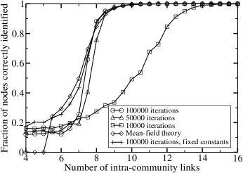
Figure 1: Accuracy of belief propagation and mean-field algorithms. Circles, squares, and triangles represent different numbers of iterations, using constants from Eq. (3). Pluses represent a different, fixed choice of constants described in text.

The results of this procedure are shown in Fig. 1. As seen, with 100000 iterations, the algorithm is highly accurate. With 50000 iterations, a slight decrease in accuracy is noticed for small $z_{in}$, and the accuracy goes down significantly at $10000$ iterations (by increasing to $200000$ iterations, a slight improvement is noted for $z_{in}<8$). For the first three curves, we used the choice of constants in Eq. (3). Since these constants depend on the given $z_{in},z_{out}$, something which may not be known for an arbitrary network, we repeated the algorithm with a particular fixed choice of constants, $\exp[J]=6,\exp[NJ^{\prime}]=10^{-10}$. This choice of constants was chosen completely arbitrarily, but as seen the algorithm still works well, with a much higher accuracy than the Newman-Girvan algorithm. However, the Newman-Girvan algorithm has some advantages in terms of picking the most optimal number of different communities into which to divide the network, while the present algorithm takes the number of communities as an input. We ignore, however, the a priori knowledge that each community has 32 nodes.

Finally, we have tested the mean-field algorithm. As seen, this is almost as accurate as the belief propagation algorithm for $z_{in}\geq 8$, and actually performs better for $z_{in}\leq 7.5$. We believe that the improved performance is a result of the fact that the mean-field equations more easily break symmetry. Tests on networks with a lower coordination number showed the difference more clearly, as given in Fig. 2 for a network with four groups and $z_{in}+z_{out}=4$.

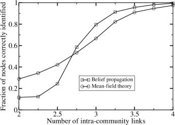
Figure 2: Accuracy of belief propagation and mean-field algorithms for $z_{in}+z_{out}=4$.

We have also tested the belief propagation algorithm on simple networks, such as dividing $N$ nodes arranged on a straight line with connections between nearest neighbors on the line into two different communities, as well as the Zachary karate club networkzach . The relaxation of the algorithm needed to be done slightly more slowly than described above (ten randomly chosen nodes were relaxed before each edge was relaxed), and some care was taken on the constants due to the lower coordination number in order to obtain convergence: with poor choices the beliefs $p_{i}(r)$ oscillated randomly. After finding these constants on the straight line network, the algorithm was tested on the Zachary network, and identified the communities accurately, with one error of placing node $10$ in the wrong community, as labeled in the figure in ng . However, this node has one link to each of the two communities and so the network gives nodes no obvious preference for either community. Interestingly, after convergence of the equations, for almost all nodes $i$, the maximum over $r$ of $p_{i}(r)$ was greater than $0.99$, except node $9$ where it was only $0.98$ and node $10$ where it was only $0.87$; these two nodes have roughly equal connections to both communities.

Discussion— We have expressed community detection as an inference problem, providing a formulation of the problem in statistical mechanical terms. We have then applied the belief propagation method to solve the resulting statistical problem. The results are accurate, however there are a number of questions that should be addressed as well as possible extensions. First, there is some questions about picking the constants $J,J^{\prime}$. In some cases, especially on test networks with a low coordination number, a poor choice of constants leads to either a lack of convergence of the belief propagation equations, or else convergence to a solution in which $p_{i}(r)\rightarrow 1/q$ so that the spontaneous symmetry breaking is absent. In both cases the algorithm performs poorly at finding the communities. The former case requires a slower relaxation of the equations, while the latter case requires an increase in the constants $J,J^{\prime}$. Fortunately, both of these cases can be detected by looking at the $p_{i}(r)$ as the algorithm runs, and then corrected, so that the algorithm warns of its possible failure in these cases. We did not find any case in which the belief propagation equations converged to a poor solution which spontaneously broke symmetry.

The next question is the scaling of the algorithm with system size. Accurate results were found with $50000$ iterations. Since each iteration updates one directed edge, there are roughly $50000/(128*16)\approx 24$ iterations per edge. Even with $10000$ iterations, or roughly $5$ per edge, some information is found. For a general network, we expect that if there are few links between communities, then the number of iterations required per edge will be proportional to the phase-ordering time for a given community under the appropriate dynamics. This phase ordering time typically scalespho as some power of the relevant length scale for a community, and for many networks this length scale is of order $\log(N)$. We thus expect for a network with average coordination number $z$ that the time will typically be of order $zN\log(N)^{\alpha}$ for some $\alpha$.

There are a number of possible ways of modifying the algorithm, also. It may be desirable to incorporate additional a priori knowledge about the communities, or to study the modularity of the different divisions, as in ng . In some cases, the belief propagation equations may be reduced to linear programminglp . A final interesting question relates to our need for spontaneous symmetry breaking. It would be desirable to be able to go beyond belief propagation using methods such as loopex . However, doing this may cause us to lose the symmetry breaking, and thus the MAP approximation may need to be replaced. Survey propagationsurvey may help in this regard, as it allows us to consider a distribution of magnetic fields for each site, each possibility corresponding to a different symmetry breaking. Even without these extensions, however, the present algorithm leads to useful results.

Acknowledgements— I thank M. Chertkov and E. Ben-Naim for useful discussions. This work was supported by US DOE W-7405-ENG-36.

References

- (1) M. E. J. Newman, Eur. Phys. J B 38, 321 (2004).
- (2) R. Guimerà et. al., Phys. Rev. E 68, 065103; P. Holme, M. Huss, and H. Jeong, Bioinformatics 19, 532 (2003).
- (3) For a variety of methods, see references in L. Deon et. al., J. Stat. P09008 (2005).
- (4) M. E. J. Newman and M. Girvan, Phys. Rev. E 69, 026113 (2004).
- (5) J. Reichardt and S. Bornholdt, Phys. Rev. Lett. 93, 218701 (2004); J. Reichardt and S. Bornholdt, preprint cond-mat/0603718.
- (6) R. G. Gallager, Low density parity check codes (MIT Press, Cambridge, MA, 1963).
- (7) D. J. C. MacKay, Information Theory, Inference, and Learning Algorithms (Cambridge University Press, Cambridge, 2003).
- (8) N. Sourlas, Nature 339, 29 (1989).
- (9) H. A. Bethe, Proc. Roy. Soc. London A 150, 552 (1935); R. Peierls, Proc. Camb. Phil. Soc 32, 477 (1936).
- (10) M. E. J. Newman, Phys. Rev. E 69, 066133 (2004).
- (11) W. W. Zachary, Jour. Anthrop. Res. 33, 452 (1977).
- (12) M. Chertkov and M. G. Stepanov, preprint cs.IT/0601113.
- (13) A. J. Bray, Adv. Phys. 43, 357 (1994).
- (14) M. Chertkov and V. Y. Chernyak, preprint cond-mat/0603189; M. Chertkov and V. Y. Chernyak, preprint cond-mat/0601487.
- (15) M. Mezard, G. Parisi, and R. Zecchina, Science 297, 812 (2002).