Theory of helimagnons in itinerant quantum systems II:
Nonanalytic corrections to Fermi-liquid behavior

Abstract

A recent theory for the ordered phase of helical or chiral magnets such as MnSi is used to calculate observable consequences of the helical Goldstone modes or helimagnons. In systems with no quenched disorder, the helimagnon contributions to the specific heat coefficient is shown to have a linear temperature dependence, while the quasi-particle inelastic scattering rate is anisotropic in momentum space and depends on the electronic dispersion relation. For cubic lattices the generic temperature dependence is given by a non-Fermi-liquid $T^{3/2}$ behavior. The contribution to the temperature dependence of the resistivity is shown to be $T^{5/2}$ in a Boltzmann approximation. The helimagnon thus leads to nonanalytic corrections to Fermi-liquid behavior. Implications for experiments, and for transport theories beyond the Boltzmann level, are discussed.

I Introduction

The itinerant helical magnet MnSi has attracted a considerable amount of interest lately. This material shows, at ambient pressure, helical magnetic order below a critical temperature $T_{c}\approx 30\,{\text{K}}$.Ishikawa et al. (1976) The wavelength of the helix is $2\pi/q$, with $q\approx 0.035\,\text{\AA}$ the pitch wave number.Ishikawa et al. (1976) Application of hydrostatic pressure $p$ monotonically decreases $T_{c}$ until $T_{c}$ vanishes at $p=p_{c}\approx 14\,\text{kbar}$.Pfleiderer et al. (1997) A tricritical point is observed on the phase boundary at $T\approx 10\,\text{K}$, such that the paramagnetic-to-helimagnetic transition at higher pressures and lower temperatures is of first order, while the transition at lower pressures and higher temperatures is of second or very weakly first order.Pfleiderer et al. (1997, 2001) In the ordered phase, neutron scattering shows the helical pattern of the magnetization with the axis of the helix pinned in the $[111]$-direction due to crystal field effects.Ishikawa and Arai (1984) In the disordered phase, quasi-static remnants of helical order are still observed at low temperatures close to the phase boundary. The distribution of the helical axis orientation is much more isotropic than in the ordered phase, with broad maxima in the $[110]$-direction.Pfleiderer et al. (2004) Such remnants of order in the disordered phase are not entirely unexpected close to a first order phase transition boundary.Chaikin and Lubensky (1995) In the entire disordered phase, up to a temperature of a few Kelvin, and up to the highest pressures investigated ($\approx 2p_{c}$), pronounced non-Fermi-liquid behavior of the resistivity is observed, with the temperature dependence of the resistivity given by $\rho(T\rightarrow 0)\sim{\text{const.}}+T^{3/2}$.Pfleiderer et al. (2001) In the ordered phase, on the other hand, the transport is observed to be Fermi-liquid-like, with a leading $T^{2}$-dependence of the resistivity. No explanation has been given so far for the unusual properties in the disordered phase. However, it is natural to speculate that the remnants of the helical order that are clearly observed in the paramagnetic phase have something to do with them. As a first step in investigating this possibility, the effects of the helical magnetic order on the electronic properties in the ordered phase of an itinerant electron system need to be understood.

In a previous paper, hereafter denoted by I, we presented a theory for the long-ranged order and fluctuations in the helically ordered phase of itinerant chiral magnets.Belitz et al. (2006) In particular, we obtained the helical Goldstone modes or helimagnons in the ordered phase. Physical quantities computed included the leading contribution to the dynamical magnetic susceptibility at wave numbers near the helical pitch wave number, and the noninteracting single-particle Green function in the ordered phase. Results for the helimagnon consistent with I were obtained in Ref. Maleyev, .

In the present paper we use the results of I to determine some of the thermodynamic and transport properties of the helical magnetic state. In particular we will calculate the effects of the magnetic fluctuations in the ordered phase on the specific heat coefficient and on the electrical resistivity to first order in these fluctuations. We will see that the magnetic soft modes lead to nonanalytic corrections to the standard Fermi-liquid theory results. Specifically, we find that the specific heat coefficient $\gamma$ has a contribution linear in the temperature $T$, whereas Fermi-liquid theory gives a leading correction to the constant Pauli value that is proportional to $T^{2}\ln T$. Similarly, the resistivity we find to have a $T^{5/2}$ term while Fermi-liquid theory gives a $T^{3}$ correction to the leading $T^{2}$ contribution. Finally, the quasi-particle or inelastic relaxation rate has a temperature dependence proportional to $T^{3/2}$, which is stronger than the $T^{2}$ behavior found in Fermi-liquid theory. Similar effects in metallic antiferromagnets, in particular an anomalously large scattering rate, have been discussed in Ref. Irkhin and Katsnelson, 2000

The plan of this paper is as follows. In Section II we give simple physical plausibility arguments that show how our results arise and how they are related to the behavior of more familiar systems. In Section III the results are derived using a combination of field theory, many-body perturbation theory, and transport theory. In Section IV we further discuss our results and their experimental implications.

II Simple physical arguments, and results

In this Section we use simple physical arguments to obtain some of our results and discuss certain aspects of them. More detailed and thorough technical derivations will be given in later sections.

II.1 Specific heat

In I we showed that in the chiral magnetic state there is one Goldstone mode, the helimagnon. Denoting the frequency of the helimagnon by $\omega_{0}$ and the wave vector by ${\bm{k}}$, the dispersion relation in the long-wavelength limit is given byrot

$$\omega_{0}({\bm{k}})=\sqrt{c_{z}k_{z}^{2}+c_{\perp}{\bm{k}}_{\perp}^{4}},$$ (1)

where $c_{z}$ and $c_{\perp}$ are elastic constants which can be expressed in terms of the exchange splitting, the pitch wave number, and the Fermi wave number. The wave vector ${\bm{k}}=({\bm{k}}_{\perp},k_{z})$ has been separated into longitudinal and transverse components with respect to the pitch wave vector ${\bm{q}}=(0,0,q)$, which we take to point in the $z$-direction. Notice that this dispersion relation is strongly anisotropic, and softer in the direction transverse to the pitch vector, $\omega_{0}\sim{\bm{k}}_{\perp}^{2}$ for $k_{z}=0$, than in the $z$-direction, $\omega_{0}\sim k_{z}$ for $k_{\perp}\equiv|{\bm{k}}_{\perp}|=0$.

To the extent that the helimagnon is a well-defined quasi-particle, one expects its contribution to the internal energy density to be

$$u(T)=\frac{1}{V}\sum_{\bm{p}}\,\omega_{0}({\bm{p}})\,n(\omega_{0}({\bm{p}})).$$ (2)

Here $n(x)=1/(\exp(x/T)-1)$ is the Bose distribution function. $V$ denotes the system volume, and throughout this paper we use units such that $k_{\text{B}}=\hbar=1$. By using Eq. (1) and scaling out the temperature it is easy to see that the leading helimagnon contribution to the specific heat, $C=\partial u/\partial T$, is proportional to $T^{2}$.LRO Adding the leading Fermi liquid contribution, which is linear in $T$, the low-temperature specific heat in the helical phase is

$$C(T\to 0)=\gamma\,T+\gamma_{2}\,T^{2}+O(T^{3}\ln T).$$ (3)

Here $\gamma$ is the usual Fermi-liquid specific heat coefficient, and $\gamma_{2}$ is the coefficient of the leading helimagnon contribution. From Eq. (2) we obtain

$$\gamma_{2}=\frac{3\,\zeta(3)}{4\pi}\,\frac{1}{\sqrt{c_{z}c_{\perp}}}\ ,$$ (4)

with $\zeta(x)$ denoting the Riemann zeta-function. The term of $O(T^{3}\ln T)$ in Eq. (3) is the usual nonanalytic term in Fermi-liquid theory that also exists in a nonmagnetic metal.Baym and Pethick (1991)

It is also interesting to compare the helimagnon contribution to the specific heat contribution from the Goldstone modes or spin waves in antiferromagnets and ferromagnets, which have dispersion relations $\omega_{0}({\bm{p}})\propto|{\bm{p}}\,|$ and $\omega_{0}({\bm{p}})\propto{\bm{p}}^{\,2}$, respectively. Equation (2) yields $C_{\text{afm}}\propto T^{3}$ and $C_{\text{fm}}\propto T^{3/2}$ for these two cases.Kittel (1996) The helimagnetic case is thus in between the ferromagnetic and antiferromagnetic cases, as one would expect based on the nature of the respective Goldstone modes.

II.2 Quasi-particle relaxation rate, and electrical resistivity

The other main result of the present paper concerns the temperature dependence of the quasi-particle relaxation rate and the electrical resistivity due to the scattering of electrons by helimagnons in a helically ordered magnetic state.

II.2.1 Quasi-particle relaxation rate

To make plausible our result for the quasi-particle relaxation rate, let us recall the case of electrons with an energy-momentum relation $\epsilon_{\bm{k}}$ that are scattered by an effective dynamical potential $V({\bm{p}},i\Omega_{n})$, with ${\bm{p}}$ a momentum and $\Omega_{n}=2\pi Tn$ a bosonic Matsubara frequency. The quasi-particle relaxation rate is given by the imaginary part of the self energy, and to lowest order in the potential the latter is given by the diagram shown in Fig. 1.

Figure 1: The lowest-order electronic self energy $\Sigma$ in terms of the potential $V$ (dashed line) and the electronic Green function (solid line).

A standard calculation yields the following relaxation rate for a quasi-particle with wave vector ${\bm{k}}$ on the Fermi surface,

$$\frac{1}{\tau_{\bm{k}}}=\frac{1}{V}\sum_{\bm{p}}\frac{V^{\prime\prime}({\bm{p}}-{\bm{k}},\xi_{\bm{p}})}{\sinh(\xi_{\bm{p}}/T)}\ ,$$ (5)

where $V^{\prime\prime}({\bm{p}},\omega)={\text{Im}}\,V({\bm{p}},i\Omega_{n}\rightarrow\omega+i0)$ is the spectrum of the dynamical potential, and $\xi_{\bm{p}}=\epsilon_{\bm{p}}-\epsilon_{\text{F}}$ with $\epsilon_{\text{F}}$ the Fermi energy.

In the case of a Fermi liquid, the relevant effective potential is the dynamically screened Coulomb interaction, which has the property $V^{\prime\prime}({\bm{p}}\,,\omega)\propto\omega/p\,v_{\text{F}}$.Pines and Nozières (1989) The integration along the Fermi surface then gives simply a geometrical prefactor, and the temperature dependence of the relaxation rate is given by the integration over the modulus of ${\bm{p}}$,gol

$$\frac{1}{\tau_{\text{e-e}}}\propto\int_{-\infty}^{\infty}d\xi\,\frac{\xi}{\sinh(\xi/T)}\propto T^{2}.$$ (6)

Another well-known example is the scattering of electrons by acoustic phonons, in which case $V^{\prime\prime}({\bm{p}},\omega)\propto cp\,\delta(\omega-cp)$,Abrikosov et al. (1963) with $c$ the speed of sound. This leads to

$$\frac{1}{\tau_{\text{e-ph}}}\propto\frac{1}{V}\sum_{\bm{p}}cp\,\frac{\delta(cp-{\bm{p}}\cdot{\bm{k}}/m_{\text{e}})}{\sinh(cp/T)}\propto T^{3}.$$ (7)

We note that the delta-function contribution to the effective potential reflects the phonon propagator, whereas the prefactor $cp$ reflects a matrix element squared that describes the coupling between electrons and phonons.Fetter and Walecka (1971) Also, we have ignored a second contribution to the phonon propagator that leads to the same temperature dependence.

With these preliminary considerations one can make an educated guess about the helimagnon contribution to the quasi-particle scattering rate. First of all, the quantity $\xi_{\bm{p}}$, which measures the distance from the Fermi surface, needs to be generalized to reflect the existence of two non-spherical Fermi surfaces split by a Stoner gap. It follows from I Eqs. (4.13), and will be discussed in more detail in Sec. III below, that this generalization reads

$$\xi_{\bm{p}}\rightarrow\omega_{1,2}({\bm{p}})=\frac{1}{2}\,\left[\xi_{\bm{p}}+\xi_{{\bm{p}}+{\bm{q}}}\pm\sqrt{(\xi_{\bm{p}}-\xi_{{\bm{p}}+{\bm{q}}})^{2}+4\lambda^{2}}\right].$$ (8)

Here we neglect spin-orbit coupling effects which can qualitatively modify the band structure.Fischer and Rosch (2004) $\lambda$ is the exchange splitting or Stoner gap from I Eq. (4.10c). The Fermi surfaces are defined as the loci of wave vectors ${\bm{k}}$ with $\omega_{1,2}({\bm{k}})=0$. The inelastic lifetimes for quasi-particles on either Fermi surface have the same temperature-dependence, and for definiteness we will concentrate on the Fermi surface given by $\omega_{1}({\bm{k}})=0$. The effective potential will be proportional to the spin susceptibility, which in turn is known from I to be proportional to the Goldstone propagator. For power-counting purposes, the spectrum of the latter is adequately represented by (see I Eqs. (4.33))

$$\chi_{\phi\phi}^{\prime\prime}({\bm{p}},\omega)\propto\frac{1}{\omega_{0}({\bm{p}})}\,\delta\left(\omega-\omega_{0}({\bm{p}})\right)$$ (9)

Here $\phi$ is the order parameter phase defined in I (see Eqs. (3.4a), (4.17), (4.28), and (4.32b) in I). In addition, we expect the effective potential to contain a multiplicative function $g({\bm{k}},{\bm{p}})$ that describes the coupling between electrons and helimagnons, in analogy to the phonon case. Altogether we expect for the inverse lifetime of a quasi-particle with wave vector ${\bm{k}}$ on the 1-Fermi surface due to scattering by helimagnons

$$\frac{1}{\tau_{\bm{k}}} \propto \frac{1}{V}\sum_{\bm{p}}\frac{g({\bm{k}},{\bm{p}})}{\sinh(\omega_{1}({\bm{p}})/T)}\,\chi_{\phi\phi}^{\prime\prime}({\bm{p}}-{\bm{k}},\omega_{1}({\bm{p}})).$$

$$\hskip-20.0pt=\frac{1}{V}\sum_{\bm{p}}\frac{g({\bm{k}},{\bm{k}}+{\bm{p}})}{\omega_{0}({\bm{p}})\sinh(\omega_{0}({\bm{p}})/T)}\,\delta(\omega_{1}({\bm{k}}+{\bm{p}})-\omega_{0}({\bm{p}})).$$

The determination of the function $g$ requires some information about the coupling mechanism, as in the electron-phonon case. Since $\phi$ is a phase mode, one expects the physically relevant correlation function to describe the fluctuations of the gradient of $\phi$, rather than of the phase itself. This suggests $g({\bm{k}},{\bm{p}})\propto({\bm{k}}-{\bm{p}})^{2}$. Indeed, we will see in Sec. III that for free electrons, $\epsilon_{\bm{k}}=k^{2}/2m_{\text{e}}$, one has $g({\bm{k}},{\bm{k}}+{\bm{p}})\propto p_{z}^{\,2}$ for small deviations ${\bm{p}}\,$ from the Fermi surface. The ${\bm{p}}_{\perp}^{\,2}$ term is absent in this case, as it is in the helimagnon dispersion relation. At the same time, $\omega_{1}({\bm{k}}+{\bm{p}})={\bm{k}}_{\perp}\cdot{\bm{p}}_{\perp}/m_{\text{e}}$. Power counting then shows that $1/\tau_{\bm{k}}\propto T^{5/2}$ for generic points on the Fermi surface. However, for a generic $\epsilon_{\bm{k}}$ that is consistent with a cubic symmetry (as is relevant for, e.g., MnSi) one finds $g({\bm{k}},{\bm{k}}+{\bm{p}})\propto({\bm{k}}_{\perp}\cdot{\bm{p}}_{\perp})^{2}+O(k_{z}^{2})$. At the same time, $\omega_{1}({\bm{k}}+{\bm{p}})$ is modified such that the leading argument of the delta-function is no longer proportional to ${\bm{k}}_{\perp}\cdot{\bm{p}}_{\perp}$. Since, in a scaling sense, $p_{\perp}^{\,2}\sim p_{z}\sim T$,sca this reduces the power of temperature by one, and for generic points on the Fermi surface one obtains

$$\frac{1}{\tau_{\text{e-hm}}}\propto T^{3/2}$$ (11)

for the electron-helimagnon scattering contribution to the quasi-particle scattering rate. Notice that this is stronger than the standard Fermi-liquid contribution to the scattering rate, Eq. (6), but not strong enough to destroy the Fermi liquid.

Equation (LABEL:eq:2.10) also yields a qualitative result for antiferromagnets,fm_ whose Goldstone modes have an isotropic dispersion relation with $\omega_{0}({\bm{p}})\propto|{\bm{p}}\,|$. Power counting with $g({\bm{k}},{\bm{p}})\propto({\bm{k}}-{\bm{p}})^{2}$ yields $1/\tau_{\text{e-afm}}\propto T^{3}$. The temperature dependence is weaker than in the result for the helimagnet, as one would expect from the nature of the respective Goldstone modes.

II.2.2 Electrical conductivity

The quasi-particle lifetime is related to, but not the same as, the relevant time scale for the electrical conductivity $\sigma$, or the resisitivity $\rho=1/\sigma$. Technically, the conductivity is given by a four-fermion correlation function, and vertex corrections enter in addition to the self-energy contributions that determine the quasi-particle lifetime. Physically, backscattering events contribute more strongly to the resistivity than forward scattering events. This leads to a transport scattering rate $1/\tau_{\text{tr}}\propto\rho$ that is given by Eq. (5), or the first line in Eq. (LABEL:eq:2.10), with an extra factor of $({\bm{p}}-{\bm{k}})^{2}$ in the integrand. In addition, the transport rate gets averaged over the Fermi surface. In the Coulomb case this changes just the geometric prefactor, but not the temperature dependence. The Fermi-liquid contribution to the resistivity thus isLifshitz and Pitaevskii (1981)

$$\rho_{\,\text{e-e}}\propto T^{2}.$$ (12)

In the case of scattering by a propagating mode, as in the phonon and helimagnon cases, the momentum is slaved to the frequency by the delta-function, and hence the temperature dependence does change. In the phonon case, where the phonon wave number scales as $T$, one obtains the familiar Bloch-Grüneisen resultZiman (1960)

$$\rho_{\,\text{e-ph}}\propto T^{5}.$$ (13)

In the helimagnon case, the smallest (in a scaling sense) additional factor in the integrand is proportional to $({\bm{p}}-{\bm{k}})_{\perp}^{2}\sim T$, and the averaging over the Fermi surface is not important since the behavior at generic points on the Fermi surface is the leading one. We thus expect

$$\rho_{\,\text{e-hm}}\propto T^{5/2}.$$ (14)

Adding the Fermi-liquid contribution, we thus obtain for the low-temperature behavior of the resistivity in the ordered phase of a clean (no impurity scattering) helimagnet

$$\rho(T\to 0)=\rho_{2}\,T^{2}+\rho_{5/2}\,T^{5/2}+O(T^{3}),$$ (15)

with $\rho_{2}$ and $\rho_{5/2}$ temperature-independent coefficients.

For antiferromagnets the additional factor of $({\bm{p}}-{\bm{k}})^{2}$ in the integral leads to an additional factor of $T^{2}$ in the resistivity. The contributions from the Goldstone modes to the resistivity in this case is thus expected to be $\rho_{\,\text{afm}}\propto T^{5}$.Ueda (1977) Again, the behavior is weaker than in the helimagnetic case.

The above simple arguments capture the structure of the full theoretical development in Sec. III, although they ignore many subtleties that occur in the actual calculation. The result shows that helimagnon scattering, while leading to a nonanalytic temperature dependence to the resistivity, is weaker than the usual electron-electron contribution. Also, the $T^{5/2}$ contribution is one power of $T$ weaker than the observed temperature dependence in the paramagnetic phase of MnSi.Pfleiderer et al. (2001) Nevertheless, it is intriguing that it is a nonanalytic term and involves a half-integer power of the temperature. It is also intriguing that the temperature dependence of the quasi-particle rate in the helimagnetic phase is the same as the observed transport rate in the paramagnetic phase. We will come back to the possible relevance of these observations for the paramagnetic phase in Sec. IV.

III Effects of Helimagnons on Observables

In this section we use the field theory of fluctuations in the helically ordered phase developed in I to calculate the specific heat and the quasi-particle relaxation time.

III.1 Specific heat

In this subsection we calculate the contribution to the free energy from Gaussian helimagnon fluctuations and use the result to obtain the leading fluctuation contribution to the specific heat. We will reproduce the results of the simple argument given in Sec. II.

If we ignore all degrees of freedom other than the Goldstone mode $g$, we have from Eqs. I (4.33) the following Gaussian action,

$${\cal A}^{(2)}=\frac{1}{2}\sum_{\bm{p}}\sum_{i\Omega}g({\bm{p}},i\Omega)\,\Gamma({\bm{p}},i\Omega)\,g(-{\bm{p}},-i\Omega),$$ (16a)

with a vertex function,

$$\Gamma({\bm{p}},i\Omega)=-(i\Omega)^{2}+\omega_{0}^{2}({\bm{p}})+|\Omega|\,\gamma({\bm{p}}).$$ (16b)

Here, and in the remainder of this section, we suppress the integer index on Matsubara frequencies. $\omega_{0}({\bm{p}})$ is the oscillator frequency given by Eq. (1), and the damping coefficient $\gamma({\bm{p}})$ is given by Eq. I (4.33c). In this Gaussian approximation, the Goldstone mode contribution to the grand canonical potential $\Xi$ is

$$\Xi^{(2)}=-\frac{T}{V}\,\ln\int D[g]\ \exp\left(-{\cal A}^{(2)}[g]\right).$$ (17)

This gives

$$\Xi^{(2)}=\frac{T}{2V}\sum_{\bm{p}}\sum_{i\Omega}\ \ln\Gamma({\bm{p}},i\Omega).$$ (18)

Neglecting the $i\Omega=0$ term, which does not contribute to the specific heat, the frequency sum is conveniently performed by using the identity (see Appendix A)

$$T\sum_{i\Omega}\ln\Gamma({\bm{p}},i\Omega) = \frac{-T}{\pi}\int_{0}^{\infty}d\omega\,\left[\ln\sinh\frac{|\omega|}{2T}-\ln|\omega|\right]\,$$ (19)

$$\times{\text{Im}}\,\left(\frac{\partial}{\partial\omega}\,\ln\Gamma({\bm{p}},\omega+i0)\right).$$

The specific heat at constant volume is obtained from $\Xi$ via the relationC_f

$$C_{V}=-T\partial^{2}\Xi/\partial T^{2}=\frac{\partial}{\partial T}\,\left[\Xi-T\,\frac{\partial\Xi}{\partial T}\right].$$ (20)

In the limit of negligible damping, $\gamma({\bm{p}})\to 0$, the expression for $C_{V}$ can be written, by combining Eqs. (19) and (20),

$$C_{V}(T)=\frac{\partial}{\partial T}\,\frac{1}{V}\sum_{\bm{p}}\omega_{0}({\bm{p}})\,n_{B}(\omega_{0}({\bm{p}})).$$ (21)

This is identical with the result for $C_{V}$ obtained from Eq. (2), and leads to Eq. (4) for the specific heat coefficient. With a nonzero damping coefficient, the frequency integral cannot be done in closed form, but the asymptotic low-temperature behavior is still proportional to $T^{2}$.dam

The model calculation given in I, which kept modes with wave numbers $k=0$ and $k=q$, results in a helimagnon dispersion relation (see Eq. I (4.33b) and Ref. err, )

$$\omega_{0}({\bm{k}})=\lambda\,\frac{q}{3k_{\text{F}}}\sqrt{k_{z}^{2}/(2k_{\text{F}})^{2}+\frac{1}{2}\,k_{\perp}^{4}/(2qk_{\text{F}})^{2}}.$$ (22a)

Keeping modes with higher wave numbers changes the dispersion relation to

$$\omega_{0}({\bm{k}})=\lambda\,\frac{q}{3k_{\text{F}}}\sqrt{k_{z}^{2}/(2k_{\text{F}})^{2}+\frac{3}{8}\,k_{\perp}^{4}/(2qk_{\text{F}})^{2}}.$$ (22b)

This result, which is analogous to the one obtained for cholesteric liquid crystals,Lubensky (1972) leads to the following values for the elastic constants in (1),

$$c_{z} = \lambda^{2}\,q^{2}/36\,k_{\text{F}}^{4},$$ (23a)

$$c_{\perp} = \lambda^{2}/96\,k_{\text{F}}^{4}.$$ (23b)

Here $k_{\text{F}}$ is the Fermi wave number, and the energy scale $\lambda$ is the exchange splitting or Stoner gap as defined in I. This results in the following asymptotic low-temperature behavior of the helimagnon contribution to the specific heat

$$C_{V}^{\text{hm}}(T)=q^{3}\,A_{C}\,(T/T_{q})^{2},$$ (24)

with a coefficient $A_{C}=\sqrt{6}\zeta(3)/2\pi\approx 0.47$, and $T_{q}=\lambda q^{2}/6k_{\text{F}}^{2}$. Equation (24) is valid for temperatures $T\ll T_{q}$. We will provide a discussion of this result, as well as a semi-quantitative analysis, in Sec. IV.

III.2 Quasi-particle relaxation time

In this subsection we calculate the temperature dependence of the quasi-particle inelastic relaxation time in a helimagnet, i.e., the lifetime of a free-electron state on the Fermi surface due to scattering by helimagnon fluctuations. We will calculate this quantity to first order in the helimagnon susceptibility. We will use the result to determine the low-temperature behavior of the electrical resistivity.

III.2.1 Effective action

To proceed, we need an electronic action that takes into account the helical magnetic order and helical magnetic fluctuations. The starting point is an electronic action of the form

$$S[{\bar{\psi}},\psi]={\tilde{S}}_{0}[{\bar{\psi}},\psi]+\frac{1}{2}\int dx\,dy\,n_{\text{s}}^{i}(x)\,A_{ij}(x-y)\,n_{\text{s}}^{j}(y).$$ (25a)

Here $${\bar{\psi}} {\psi} \alpha n_{\text{s}}^{i}(x)={\bar{\psi}}_{\alpha}(x)\sigma^{i}_{\alpha\beta}\psi_{\beta}(x) \sigma^{i} i=1,2,3 {\bm{n}}_{\text{s}}(x) x\equiv({\bm{x}},\tau) {\bm{x}} \tau \int dx=\int_{V}d{\bm{x}}\int_{0}^{1/T}d\tau {\tilde{S}}_{0} A \Gamma_{\text{t}} c$$ and are fermionic (i.e., Grassmann-valued) fields that depend on space, time, and a spin index ; , where () denotes the Pauli matrices, are the components of the electronic spin density field . comprises the position in real space and the imaginary time , and the related integration measure is given by . contains all parts of the action other than the spin-triplet interaction. The interaction amplitude consists of a point-like Hubbard interaction with an amplitude and a chiral part with coupling constant whose origin has been explained in I,

$$A_{ij}(x-y)=\delta(x-y)\,\left[\delta_{ij}\,\Gamma_{\text{t}}+\epsilon_{ijk}\,c\,\Gamma_{\text{t}}\,\partial_{k}\right].$$ (25b)

Note that $A$ is static; it depends only on spatial position, and not on imaginary time.

The general idea is now to replace one of the spin density fields in the last term in Eq. (25a) by a classical (i.e., c-number valued) field that represents the effective field seen by the electrons due to the magnetic order. If one is just interested in incorporating static helical order, one can implement a mean-field approximation by replacing either one of the spin density fields in Eq. (25a) by its average value, $n^{2}\approx 2n\langle n\rangle-\langle n\rangle^{2}$. This yields an effective action

$$S_{0}[{\bar{\psi}},\psi]={\tilde{S}}_{0}[{\bar{\psi}},\psi]+\int dx\ {\bm{H}}_{0}({\bm{x}})\cdot{\bm{n}}_{\text{s}}({\bm{x}}),$$ (26a)

where

$${\bm{H}}_{0}({\bm{x}})=\Gamma_{\text{t}}\,\langle{\bm{n}}_{\text{s}}(x)\rangle,$$ (26b)

and we have dropped a constant contribution to the action. The remaining question regards the equation of state that determines $$\langle{\bm{n}}_{\text{s}}(x)\rangle$$. This has been given in I in a saddle-point approximation, which yields

$${\bm{H}}_{0}({\bm{x}})=\lambda\,\left(\cos({\bm{q}}\cdot{\bm{x}}),\sin({\bm{q}}\cdot{\bm{x}}),0\right),$$ (26c)

Here ${\bm{q}}$ is the pitch vector of the helix, and the amplitude $\lambda$ is determined by a generalized Stoner equation of state. $S_{0}$ is the reference ensemble action given by Eq. I (4.7a), which describes noninteracting electrons (or electrons interacting via a spin-singlet interaction only) in an effective magnetic field given by the helically modulated magnetization.

More generally, one might ask whether one can replace ${\bm{H}}_{0}$ in Eq. (26a) by a fluctuating classical field ${\bm{H}}(x)=\Gamma_{\text{t}}\,{\bm{M}}(x)$, where ${\bm{M}}(x)$ represents the spin density averaged over the quantum mechanical degrees of freedom. For the sake of presentational simplicity we will explain this procedure for an ordinary Hubbard interaction ($c=0$ in Eq. (25b) and ${\bm{q}}=0$ in Eq. (26c)). The development for the chiral interaction is exactly analogous.

Writing ${\bm{M}}(x)={\bm{H}}_{0}/\Gamma_{\text{t}}+\delta{\bm{M}}(x)$, and ignoring a constant contribution to the action, one has

$$S[{\bar{\psi}},\psi,\delta{\bm{M}}]=S_{0}[{\bar{\psi}},\psi]+\Gamma_{\text{t}}\int dx\ \delta{\bm{M}}(x)\cdot\delta{\bm{n}}_{\text{s}}(x),$$ (27a)

with $$\delta{\bm{n}}_{\text{s}}(x)={\bm{n}}_{\text{s}}(x)-\langle{\bm{n}}_{\text{s}}(x)\rangle \delta{\bm{M}} {\bm{M}}$$. This needs to be supplemented by an action governing . If the expectation value of is to represent the exact magnetization, this action must be

$${\cal A}[\delta{\bm{M}}]=-\frac{1}{2}\int dx\,dy\ \delta M_{i}(x)\,\left(\chi_{\text{s}}^{-1}\right)_{ij}(x,y)\,\delta M_{j}(y),$$ (27b)

where $\chi_{\text{s}}$ is the spin susceptibility of the system. A purely electronic effective action is now obtained by integrating out the fluctuations $\delta{\bm{M}}$. The Gaussian integral yields

$$S_{\text{eff}}[{\bar{\psi}},\psi]=S_{0}[{\bar{\psi}},\psi]+\frac{\Gamma_{\text{t}}^{2}}{2}\int dx\,dy\ \delta n_{\text{s}}^{i}(x)\,\chi_{\text{s}}^{ij}(x,y)\,\delta n_{\text{s}}^{j}(y).$$ (28)

With the full chiral interaction, Eq. (25b), one obtains formally the same result. The only reservation is that in the chiral case the correlation function $\langle\delta M\,\delta M\rangle=\chi_{\text{s}}$ is, strictly speaking, not the physical spin susceptibility. However, its leading hydrodynamic contribution is the same as that of the latter, as was shown in I. The result (28) thus consists of the reference ensemble described by $S_{0}$, whose Green function has been determined in I, and an effective interaction given by the spin susceptibility in the helically ordered phase. The latter has been calculated in I in a Gaussian approximation. Notice that the effective potential depends on imaginary time or frequency.

It is obvious that the above heuristic considerations represent, in a diagrammatic language, some kind of infinite resummation, which means that the resulting effective action is valid only in conjunction with certain constraints. To clarify this point it is useful to rewrite the starting point, Eq. (25a), in the form

$$S[{\bar{\psi}},\psi]=S_{0}[{\bar{\psi}},\psi]+\frac{1}{2}\int dx\,dy\,\delta n_{\text{s}}^{i}(x)\,A_{ij}(x-y)\,\delta n_{\text{s}}^{j}(y).$$ (29)

Now consider the bare spin-triplet interaction $A$, Fig. 2, and its renormalization by the ladder resummation shown in Fig. 3.

Figure 2: Diagrammatic representation of the bare spin-triplet interaction $A$ and the reference ensemble Green function $G$.

Figure 3: Effective spin-triplet interaction resulting from a ladder resummation.

The result of this resummation is an effective interaction of the form given in Eq. (28), with a Gaussian approximation for $\chi_{\text{s}}$. The constraint that must be used in conjunction with the effective action (28) is now obvious: The effective interaction must not be used in ways that constitute renormalizations of $\chi_{\text{s}}$, as doing so would result in double counting. In particular, it is safe to use Eq. (28) in any perturbative calculation to linear order in $\chi_{\text{s}}$. We will now proceed and use it to calculate the quasi-particle inelastic lifetime to that order.

III.2.2 Electronic self energy and Green function

We consider the self energy $\Sigma$ of the single-particle Green function to first order in the perturbing potential $\Gamma_{\text{t}}^{2}\,\chi_{\text{s}}\equiv{\tilde{\chi}}_{\text{s}}$. There are two self-energy diagrams to this order, namely, the direct or Hartree and the exchange or Fock contributions shown in Figs. 4(a) and 4(b), respectively.

Figure 4: The direct (a) and exchange (b) contributions to the single-particle self energy.

Both self-energy contributions are nondiagonal in both spin and momentum space. It is readily seen that the direct contribution is purely real, and hence does not contribute to the scattering rate. The exchange contribution is given by,

$$\Sigma^{\,\text{ex}}_{\,{\bm{k}}{\bm{p}}}(i\omega) = \frac{1}{V}\sum_{{\bm{k}}^{\prime},{\bm{p}}^{\prime}}T\sum_{i\Omega}\sigma^{i}\,G_{{\bm{k}}^{\prime}+{\bm{k}},{\bm{p}}^{\prime}+{\bm{p}}}(i\Omega+i\omega)\,\sigma^{j}\,$$ (30)

$$\hskip 40.0pt\times{\tilde{\chi}}_{\text{s}}^{ij}({\bm{k}}^{\prime},{\bm{p}}^{\prime};i\Omega).$$

Here $i\omega$ denotes a fermionic Matsubara frequency, and $G_{{\bm{k}}{\bm{p}}}(i\omega)$ is the single-particle Green function of the reference ensemble which is given explicitly by Eqs. I (4.13). All components of the self energy can be obtained from Eq. (30) by means of straightforward, albeit lengthy, calculations.

We now consider the Dyson equation for the renormalized Green function ${\cal G}$, which reads

$${\cal G}^{-1}_{{\bm{k}}{\bm{p}}}(i\omega)=G^{-1}_{{\bm{k}}{\bm{p}}}(i\omega)-\Sigma_{\,{\bm{k}}{\bm{p}}}(i\omega).$$ (31)

From Eqs. I (4.13) for $G$ and Eq. (30) it follows that $\Sigma$ has a structure very similar to that of $G^{-1}$,

$$\Sigma_{\,{\bm{k}}{\bm{p}}}(i\omega) = \delta_{{\bm{k}}{\bm{p}}}\,\left[\sigma_{+-}\,\Sigma_{++}({\bm{k}},i\omega)+\sigma_{-+}\,\Sigma_{--}({\bm{k}},i\omega)\right]$$ (32)

$$+\,\delta_{{\bm{k}}+{\bm{q}},{\bm{p}}}\,\sigma_{+}\,\Sigma_{+-}({\bm{k}},i\omega)$$

$$+\,\delta_{{\bm{k}}-{\bm{q}},{\bm{p}}}\,\sigma_{-}\,\Sigma_{-+}({\bm{k}},i\omega).$$

Here the notation is the same as in Eqs. I (4.13). In particular, $\sigma_{\pm}=(\sigma_{1}\pm i\sigma_{2})/2$, $\sigma_{+-}=\sigma_{+}\sigma_{-}$, and $\sigma_{-+}=\sigma_{-}\sigma_{+}$, with $\sigma_{1,2}$ Pauli matrices. From this expression it follows in turn that ${\cal G}$ has the same structure as $G$,

$${\cal G}_{{\bm{k}}{\bm{p}}}(i\omega) = \delta_{{\bm{k}}{\bm{p}}}\,\bigl{[}\sigma_{+-}\,A_{+}({\bm{k}},i\omega)+\sigma_{-+}\,A_{-}({\bm{k}},i\omega)\bigr{]}$$ (33a)

$$+\,\delta_{{\bm{k}}+{\bm{q}},{\bm{p}}}\,\sigma_{+}\,B_{+}({\bm{k}},i\omega)$$

$$+\,\delta_{{\bm{k}}-{\bm{q}},{\bm{p}}}\,\sigma_{-}\,B_{-}({\bm{k}},i\omega).$$

Here

$$A_{\pm}({\bm{k}},i\omega) = \frac{g^{-1}_{\mp}({\bm{k}}\pm{\bm{q}},i\omega)}{g^{-1}_{\mp}({\bm{k}}\pm{\bm{q}},i\omega)\,g^{-1}_{\pm}({\bm{k}},i\omega)-\left(\lambda_{\pm}({\bm{k}},i\omega)\right)^{2}}$$

$$B_{\pm}({\bm{k}},i\omega) = \frac{-\lambda_{\pm}({\bm{k}},i\omega)}{g^{-1}_{\mp}({\bm{k}}\pm{\bm{q}},i\omega)\,g^{-1}_{\pm}({\bm{k}},i\omega)-\left(\lambda_{\pm}({\bm{k}},i\omega)\right)^{2}}$$

with

$$g^{-1}_{\pm}({\bm{k}},i\omega)=G^{-1}({\bm{k}},i\omega)-\Sigma_{\pm\pm}({\bm{k}},i\omega),$$ (33d)

$$\lambda_{\pm}({\bm{k}},i\omega)=\lambda-\Sigma_{\pm\mp}({\bm{k}},i\omega).$$ (33e)

These expressions constitute an exact inverse of Eq. (31), as can easily be checked by a direct multiplication.

III.2.3 Quasi-particle relaxation time

The quasi-particle relaxation time is determined by the imaginary parts of the poles of the Green function ${\cal G}$, Eqs. (33). For a vanishing self energy there are poles at

$$\omega_{1,2}^{\pm}({\bm{k}})=\frac{1}{2}\,\left(\xi_{\bm{k}}+\xi_{{\bm{k}}\pm{\bm{q}}}\pm\sqrt{\left(\xi_{\bm{k}}-\xi_{{\bm{k}}\pm{\bm{q}}}\right)^{2}+4\lambda^{2}}\right),$$

with $\xi_{\bm{k}}$ as defined after Eq. (5). The poles with different signs of the square root reflect the Stoner splitting of the Fermi surface into two sheets. On a given sheet, $\omega^{+}$ and $\omega^{-}$ are related by $\omega_{i}^{-}({\bm{k}}+{\bm{q}})=\omega_{i}^{+}({\bm{k}})$ ($i=1,2$). All poles can thus be expressed in terms of

$$\omega_{1,2}({\bm{k}})=\frac{1}{2}\,\left(\xi_{\bm{k}}+\xi_{{\bm{k}}+{\bm{q}}}\pm\sqrt{\left(\xi_{\bm{k}}-\xi_{{\bm{k}}+{\bm{q}}}\right)^{2}+4\lambda^{2}}\right).$$ (34)

Both of these resonance frequencies are real, reflecting the fact that the quasi-particles are infinitely long lived to zeroth order in the effective potential $\chi_{\text{s}}$. To first order in $\chi_{\text{s}}$ the resonance frequencies acquire an imaginary part, corresponding to a finite relaxation time $\tau({\bm{k}})$, in addition to a shift of the real part. For definiteness, we consider the resonance at $\omega_{1}({\bm{k}})$; the relaxation time on the other sheet has the same temperature dependence. We find

$$\frac{1}{\tau({\bm{k}})} = {\text{Im}}\left\{\Sigma_{++}({\bm{k}},z)+\Sigma_{--}({\bm{k}}+{\bm{q}},z)+\frac{(\xi_{\bm{k}}-\xi_{{\bm{k}}+{\bm{q}}})}{\left[\left(\xi_{\bm{k}}-\xi_{{\bm{k}}+{\bm{q}}}\right)^{2}+4\lambda^{2}\right]^{1/2}}\,\left[\Sigma_{++}({\bm{k}},z)-\Sigma_{--}({\bm{k}}+{\bm{q}},z)\right]\right.$$ (35)

$$\hskip 20.0pt\left.-\frac{2\lambda}{\left[\left(\xi_{\bm{k}}-\xi_{{\bm{k}}+{\bm{q}}}\right)^{2}+4\lambda^{2}\right]^{1/2}}\,\left[\Sigma_{+-}({\bm{k}},z)+\Sigma_{-+}({\bm{k}}+{\bm{q}},z)\right]\right\}\ .$$

Here the frequency $z$ is given by the ‘on-shell condition’ $z=\omega_{1}({\bm{k}})+i0$.

Of particular interest is the relaxation rate for quasi-particles on the Fermi surface, which is defined by

$$\omega_{1}({\bm{k}}) = \frac{1}{2}\,\left(\xi_{\bm{k}}+\xi_{{\bm{k}}+{\bm{q}}}+\left[\left(\xi_{\bm{k}}-\xi_{{\bm{k}}+{\bm{q}}}\right)^{2}+4\lambda^{2}\right]^{1/2}\right)$$ (36a)

$$= 0.$$

For $$\lambda={\bm{q}}=0 \xi_{\bm{k}}=0$$ this reduces to the usual definition of the Fermi surface, . In the general case it implies in particular

$$\xi_{\bm{k}}\,\xi_{{\bm{k}}+{\bm{q}}}=\lambda^{2}.$$ (36b)

With this condition, we use Eq. (30) in Eq. (35), and the results of I for $\chi_{\text{s}}$, keeping only the leading hydrodynamic contributions to the latter. Performing the frequency summations we find for the relaxation rate of a quasi-particle on the Fermi surface

$$\frac{1}{\tau_{\text{F}}({\bm{k}})} = \frac{-2\lambda^{2}}{\left(\xi_{\bm{k}}+\xi_{{\bm{k}}+{\bm{q}}}\right)^{2}}\,\frac{1}{V}\sum_{\bm{p}}\ \frac{g({\bm{k}},{\bm{p}})}{\sinh\left(\omega_{1}({\bm{p}})/T\right)}\$$ (37a)

$$\hskip 40.0pt\times\chi_{\phi\phi}^{\prime\prime}\left({\bm{p}}-{\bm{k}},\omega_{1}({\bm{p}})\right).$$

This expression is valid to determine the leading low-temperature behavior of $$1/\tau_{\text{F}} {\bm{p}}\approx{\bm{k}} {\bm{p}} {\bm{k}} {\bm{p}}\to{\bm{k}} \chi_{\phi\phi}^{\prime\prime} \phi$$ only. We have anticipated the fact that the dominant contribution to the latter comes from momenta , and accordingly have replaced by in all contributions to the integrand that have a finite and nonzero limit as . Here is the spectrum of the susceptibility of the phase fluctuation variable that was introduced in I. Its leading hydrodynamic part is also proportional to the Goldstone mode. From I (4.33a) or, alternatively, from I (4.29a) and (4.40),err we find for the phase susceptibility

$$\chi_{\phi\phi}({\bm{p}},i\Omega)=\frac{1}{2N_{\text{F}}}\,\frac{q^{2}}{3k_{\text{F}}^{2}}\,\frac{1}{\omega_{0}^{2}({\bm{p}})-(i\Omega)^{2}}\ ,$$ (37b)

where $$\omega_{0}({\bm{p}})$$ is the helimagnon resonance frequency, see Eqs. (1) and I (4.33b). The spectrum is thus

$$\chi_{\phi\phi}^{\prime\prime}({\bm{p}},\omega) = \frac{1}{2N_{\text{F}}}\,\frac{q^{2}}{3k_{\text{F}}^{2}}\,\frac{\pi}{2\omega_{0}({\bm{p}})}\bigl{[}\delta\left(\omega-\omega_{0}({\bm{p}})\right)$$ (37c)

$$\hskip 50.0pt-\delta\left(\omega+\omega_{0}({\bm{p}})\right)\bigr{]}.$$

The function $$g$$ is given by

$$g({\bm{k}},{\bm{p}}) = \omega_{1}({\bm{p}})\left(\xi_{\bm{k}}+\xi_{{\bm{k}}+{\bm{q}}}\right)+\xi_{\bm{k}}\left(\xi_{{\bm{k}}+{\bm{q}}}-\xi_{{\bm{p}}+{\bm{q}}}\right)\hskip 30.0pt$$ (37d)

$$\hskip 78.0pt+\xi_{{\bm{k}}+{\bm{q}}}\left(\xi_{\bm{k}}-\xi_{\bm{p}}\right)\ .$$

Notice that $g({\bm{k}},{\bm{k}})=0$, that $\chi^{\prime\prime}({\bm{p}},\omega)$ is soft at ${\bm{p}}=0$ and $\omega=\omega_{1}({\bm{k}})=0$, and that Eq. (37a) has indeed the form of the educated guess, Eq. (LABEL:eq:2.10).

For later reference we also introduce the ‘off-shell’ rate $1/\tau({\bm{k}},\epsilon)$ obtained by putting $z=\epsilon+i0$ in the self energies in Eq. (35). With ${\bm{k}}$ on either Fermi surface one finds

$$\frac{1}{\tau_{i}({\bm{k}},\epsilon)}=\frac{-2\pi\lambda^{2}}{\left(\xi_{\bm{k}}+\xi_{{\bm{k}}+{\bm{q}}}\right)^{2}}\int\frac{du}{\pi}\,\left[n(u)+f(\epsilon+u)\right]\,\frac{1}{V}\sum_{\bm{p}}g_{i}({\bm{k}},{\bm{p}}\,;\epsilon)\,\chi_{\phi\phi}^{\prime\prime}({\bm{p}}-{\bm{k}},u)\,\delta\left(u+\epsilon-\omega_{i}({\bm{p}})\right),\quad(i=1,2)\ ,$$ (38a)

Here $$\omega_{i}({\bm{p}})$$ is given by Eq. (34), and

$$g_{i}({\bm{k}},{\bm{p}}\,;\epsilon)=\left(\omega_{i}({\bm{p}})-\xi_{\bm{p}}\right)(\xi_{{\bm{k}}+{\bm{q}}}-\epsilon)-\left(\omega_{i}({\bm{p}})-\xi_{{\bm{p}}+{\bm{q}}}\right)\,\frac{\xi_{\bm{k}}\xi_{{\bm{k}}+{\bm{q}}}}{\epsilon-\xi_{{\bm{k}}+{\bm{q}}}}+2\xi_{\bm{k}}\,\xi_{{\bm{k}}+{\bm{q}}}$$ (38b)

is a generalization of Eq. (37d), with the property $g_{1}({\bm{k}},{\bm{p}}\,;\epsilon=0)=g({\bm{k}},{\bm{p}})$.

To evaluate the final integral we consider the limit $\epsilon_{\text{F}}\gg\lambda\gg qv_{\text{F}}$, as we did in I. The result will obviously depend on the direction of ${\bm{k}}$. It also depends on the functional form electronic energy momentum relation $\epsilon_{\bm{k}}$.

Isotropic energy-momentum relation

Let us first consider a nearly-free electron approximation, with

$$\epsilon_{\bm{k}}={\bm{k}}^{2}/2m_{\text{e}},$$ (39)

with $m_{\text{e}}$ the effective mass of the electrons. Then $g({\bm{k}},{\bm{k}}+{\bm{p}})\propto p_{z}^{2}+O(p_{z}^{3})$, and $\omega_{1}({\bm{k}}+{\bm{p}})={\bm{k}}_{\perp}\cdot{\bm{p}}_{\perp}/m_{\text{e}}+O(k_{z}p_{z},k_{\perp}^{2})$.

For ${\bm{k}}_{\perp}=0$ the leading result as $T\to 0$ is

$$\frac{1}{\tau(\bm{k})} = \pi^{3}\sqrt{6}\ \frac{\lambda q^{4}}{m_{\text{e}}^{2}}\,\frac{k_{\text{F}}^{3}}{k_{z}^{3}}\,\frac{T^{2}}{(\xi_{\bm{k}}+\xi_{{\bm{k}}+{\bm{q}}})^{4}}$$ (40a)

$$\propto \lambda\left(\frac{q}{k_{\text{F}}}\right)^{8}\left(\frac{\epsilon_{\text{F}}}{\lambda}\right)^{2}\left(\frac{T}{T_{q}}\right)^{2},$$

with $$T_{q} {\bm{k}}_{\perp}\neq 0$$ the temperature scale defined after Eq. (24). For the asymptotic result is

$$\frac{1}{\tau(\bm{k})} = A_{\tau}\,\frac{\lambda^{1/2}qk_{\text{F}}^{3}}{m_{e}^{2}}\,\frac{k_{\text{F}}}{k_{\perp}}\,\frac{T^{5/2}}{(\xi_{\bm{k}}+\xi_{{\bm{k}}+{\bm{q}}})^{4}}$$ (40b)

$$\propto \lambda\,\left(\frac{q}{k_{\text{F}}}\right)^{6}\left(\frac{\epsilon_{\text{F}}}{\lambda}\right)^{2}\left(\frac{T}{T_{q}}\right)^{5/2}.$$

with $A_{\tau}\approx 289$. In the second lines in Eqs. (40a) and (40b) we have assumed a generic value of ${\bm{k}}$, and have neglected all numerical prefactors as well as terms small in $qv_{\text{F}}/\lambda$ for clarity. The crossover between these two types of behavior occurs at a temperature proportional to $T_{\times}=\lambda\,(q/k_{{\text{F}}})^{6}(k_{\perp}/k_{z})^{2}$. It is easy to check that adding an isotropic quartic term, proportional to $({\bm{k}}^{2})^{2}$, to $\epsilon_{\bm{k}}$ does not change the powers of the temperature in these results.

Cubic energy-momentum relation

In an actual metal, the underlying lattice structure causes the electronic energy-momentum relation to be anisotropic. In the case of a cubic lattice, as in MnSi, any terms consistent with cubic symmetry are allowed. For instance, to quartic order in ${\bm{k}}$ the following function is allowed,

$$\epsilon_{\bm{k}}={\bm{k}}^{2}/2m_{\text{e}}+\frac{\nu}{2m_{\text{e}}k_{\text{F}}^{2}}\,(k_{x}^{2}k_{y}^{2}+k_{y}^{2}k_{z}^{2}+k_{z}^{2}k_{x}^{2}),$$ (41)

with $\nu$ a dimensionless measure of deviations from a nearly-free electron model. Generically, once expects $\nu=O(1)$. Other quartic terms that are consistent with a cubic symmetry, e.g., the cubic anisotropy $k_{x}^{4}+k_{y}^{4}+k_{z}^{4}$, can be obtained by adding an isotropic $({\bm{k}}^{2})^{2}$ term to Eq. (41). For $\nu\neq 0$ the asymptotic behavior of $g$ is changed compared to the nearly-free electron case,

$$g({\bm{k}},{\bm{k}}+{\bm{p}}) = -\left(\frac{2\nu}{2m_{\text{e}}k_{\text{F}}^{2}}\right)^{2}\,\frac{\lambda^{2}\,q^{2}\,(2k_{z}+q)^{2}}{(\xi_{\bm{k}}+\xi_{{\bm{k}}+{\bm{q}}})^{2}}\,({\bm{k}}_{\perp}\cdot{\bm{p}}_{\perp})^{2}$$ (42)

$$+O(p_{\perp}p_{z})$$

and for ${\bm{q}}$ in $(0,0,1)$-direction one has

$$\omega_{1}({\bm{k}}+{\bm{p}}) = ({\bm{k}}_{\perp}\cdot{\bm{p}}_{\perp})/\mu_{\text{e}}$$ (43a)

$$+\frac{2\nu}{2m_{\text{e}}k_{{\text{F}}}^{2}}\,(k_{y}^{2}+k_{z}^{2}+k_{z}q+q^{2}/2)k_{x}p_{x}$$

$$+\frac{2\nu}{2m_{\text{e}}k_{{\text{F}}}^{2}}\,(k_{x}^{2}+k_{z}^{2}+k_{z}q+q^{2}/2)k_{y}p_{y}$$

$$+O(p_{\perp}^{2},p_{z}),$$

where

$$1/\mu_{\text{e}}=1/m_{\text{e}}+\nu\,\frac{q(2k_{z}+q)}{2m_{\text{e}}k_{\text{F}}^{2}}\,\frac{\xi_{\bm{k}}-\xi_{{\bm{k}}+{\bm{q}}}}{\xi_{\bm{k}}+\xi_{{\bm{k}}+{\bm{q}}}}.$$ (43b)

If we define

$$A_{x,y}=1+\frac{\nu\mu_{\text{e}}}{m_{\text{e}}k_{\text{F}}^{2}}\,(k_{y,x}^{2}+k_{z}^{2}+k_{z}q+q^{2}/2),$$ (44a)

and

$$C_{\bm{k}}=\frac{B\,\nu^{4}}{k_{\text{F}}^{5}}\,\frac{(2k_{z}+q)^{2}}{k_{\text{F}}^{2}}\,\frac{q^{3}k_{\text{F}}\mu_{\text{e}}^{3}}{m_{\text{e}}^{5}}\,\frac{\lambda^{3}}{(\xi_{\bm{k}}+\xi_{{\bm{k}}+{\bm{q}}})^{4}},$$ (44b)

with

$$B = \frac{48\sqrt{3}}{2^{1/4}3^{3/4}}\int_{0}^{\infty}dx\,dz\ \frac{x^{2}}{\sqrt{z^{2}+x^{4}}}\,\frac{1}{\sinh{\sqrt{z^{2}+x^{4}}}}$$ (44c)

$$= 54.99\ldots$$

the evaluation of Eqs. (37) now yields

$$\frac{1}{\tau({\bm{k}})} = C_{\bm{k}}\,\frac{k_{x}^{2}k_{y}^{2}(k_{x}^{2}-k_{y}^{2})^{2}}{(k_{x}^{2}A_{x}^{2}+k_{y}^{2}A_{y}^{2})^{3/2}}\,\left(\frac{T}{\lambda}\right)^{3/2}$$ (44d)

$$\propto \nu^{4}\lambda\left(\frac{q}{k_{\text{F}}}\right)^{6}\left(\frac{\epsilon_{\text{F}}}{\lambda}\right)^{2}\left(\frac{T}{T_{q}}\right)^{3/2}.$$

In a cubic system, the quasi-particle relaxation rate thus generically shows a $T^{3/2}$ behavior, except on four special lines in ${\bm{k}}$-space, $k_{x}=0$, $k_{y}=0$, and $k_{x}=\pm k_{y}$, where the prefactor of the $T^{3/2}$ vanishes and the behavior is $T^{2}$. These results are valid for ${\bm{q}}$ in $(0,0,1)$-direction. The corresponding expressions for ${\bm{q}}$ in $(1,1,1)$-direction, which is relevant for MnSi,q_f can be obtained by a corresponding rotation of ${\bm{k}}$. That is, $(k_{x},k_{y},k_{z})$ in the above expressions should be replaced by

$$k_{x} \rightarrow (k_{x}-\sqrt{3}k_{y}+\sqrt{2}k_{z})/\sqrt{6},$$

$$k_{y} \rightarrow (k_{x}+\sqrt{3}k_{y}+\sqrt{2}k_{z})/\sqrt{6},$$

$$k_{z} \rightarrow (-2k_{x}+\sqrt{2}k_{z})/\sqrt{6}.$$ (45)

It needs to be stressed that the $T^{5/2}$ and $T^{3/2}$ terms due to the helimagnons, as well as the Fermi-liquid $T^{2}$ term, all contribute to the quasi-particle relaxation rate, and which of these contributions dominate in a given temperature regime is a quantitative question. The same is true for the different contributions to the specific heat. In Sec. IV.1 we will give estimates for parameter values that are appropriate for MnSi.

III.3 Resistivity

The electrical resistivity can be obtained as the inverse of the conductivity, which in turn is given by the Kubo formula

$$\sigma_{ij}(i\Omega)=\frac{i}{i\Omega}\,\left[\pi_{ij}(i\Omega)-\pi_{ij}(i\Omega=0)\right].$$ (46a)

Here

$$\pi_{ij}(i\Omega) = -e^{2}\,T\sum_{n_{1},n_{2}}\frac{1}{V}\sum_{{\bm{k}},{\bm{p}}}v_{i}({\bm{k}})\,v_{j}({\bm{p}})\,\hskip 0.0pt$$

$$\hskip-20.0pt\times\left\langle{\bar{\psi}}_{n_{1},\sigma}({\bm{k}})\,\psi_{n_{1}+n,\sigma}({\bm{k}})\,{\bar{\psi}}_{n_{2},\sigma^{\prime}}({\bm{p}})\,\psi_{n_{2}-n,\sigma^{\prime}}({\bm{p}})\right\rangle.$$

is the current-current susceptibility tensor or polarization function, with ${\bm{v}}({\bm{k}})=\partial\epsilon_{\bm{k}}/\partial{\bm{k}}$. The average, denoted by $\langle\ldots\rangle$, is to be performed with the effective action given in Eq. (28). The simplest approximation to $\pi$ is a factorization of the four-point correlation function in Eq. (44b) into two Green functions. The difference between this simple approximation and the full polarization function is customarily expressed in terms of a vector vertex function ${\bm{\Gamma}}$ with components ${}_{i}\Gamma$,

$$\pi_{ij}(i\Omega) = -e^{2}\,T\sum_{i\omega}\frac{1}{V}\sum_{{\bm{k}},{\bm{p}}}\sum_{\alpha\beta}{{}_{i}\Gamma}^{\alpha\beta}_{{\bm{k}}{\bm{p}}}(i\omega,i\omega-i\Omega)$$ (47)

$$\hskip-40.0pt\times\sum_{{\bm{k}}^{\prime}}\sum_{\sigma}iv_{j}({\bm{k}}^{\prime})\,{\cal G}_{{\bm{k}}{\bm{k}}^{\prime}}^{\alpha\sigma}(i\omega)\,{\cal G}_{{\bm{k}}^{\prime}{\bm{p}}}^{\sigma\beta}(i\omega-i\Omega),$$

with ${\cal G}$ from Eq. (31). It is well known that care must be taken to use consistent approximations for the self energy $\Sigma$ that defines ${\cal G}$ and the vertex function.Baym and Kadanoff (1961); Kadanoff and Baym (1962) The simplest combination that fulfills the consistency requirement, which is equivalent to the Boltzmann equation for the conductivity, is a self-consistent Born approximation for the self energy,

$$\Sigma_{{\bm{k}}{\bm{p}}}^{\alpha\beta}(i\omega) = T\sum_{i\Omega}\frac{1}{V}\sum_{{\bm{k}}^{\prime}{\bm{p}}^{\prime}}\sum_{\alpha^{\prime}\beta^{\prime}}{\cal G}_{{\bm{k}}^{\prime}{\bm{p}}^{\prime}}^{\alpha^{\prime}\beta^{\prime}}(i\omega+i\Omega)\,$$ (48a)

$$\times V_{\alpha\alpha^{\prime}\!,\,\beta^{\prime}\beta}({\bm{k}}^{\prime}-{\bm{k}},{\bm{p}}\,^{\prime}-{\bm{p}}\,;i\Omega),$$

and a ladder approximation for the vertex function,

$${\bm{\Gamma}}_{{\bm{k}}{\bm{p}}}^{\alpha\beta}(i\omega,i\omega-i\Omega) = \delta_{{\bm{k}}{\bm{p}}}\,\delta_{\alpha\beta}\,iv({\bm{k}})+T\sum_{i\Omega^{\prime}}\frac{1}{V}\sum_{{\bm{k}}^{\prime}\!,\,{\bm{k}}^{\prime\prime}\!,\,{\bm{p}}^{\prime}\!,\,{\bm{p}}^{\prime\prime}}{\bm{\Gamma}}_{{\bm{k}}^{\prime\prime}{\bm{p}}^{\prime\prime}}^{\alpha^{\prime\prime}\beta^{\prime\prime}}(i\omega+i\Omega^{\prime},i\omega-i\Omega+i\Omega^{\prime})\,{\cal G}_{{\bm{k}}^{\prime\prime}{\bm{k}}^{\prime}}^{\alpha^{\prime\prime}\alpha^{\prime}}(i\omega+i\Omega^{\prime})\hskip 60.0pt$$ (48b)

$$\times\,{\cal G}_{{\bm{p}}^{\prime}{\bm{k}}^{\prime\prime}}^{\beta^{\prime}\alpha^{\prime\prime}}(i\omega-i\Omega+i\Omega^{\prime})\,\frac{1}{2}\,\left[V_{\alpha^{\prime}\alpha\,,\beta\beta^{\prime}}({\bm{k}}-{\bm{k}}^{\prime},{\bm{p}}-{\bm{p}}\,^{\prime};i\Omega^{\prime})+V_{\beta\beta^{\prime}\!,\,\alpha^{\prime}\alpha}({\bm{p}}\,^{\prime}-{\bm{p}}\,,{\bm{k}}^{\prime}-{\bm{k}};i\Omega^{\prime})\right].$$

Here $$V$$ is the potential in the effective action,

$$V_{\alpha\beta,\gamma\delta}({\bm{k}},{\bm{p}}\,;i\Omega)=\sum_{ij}\sigma^{i}_{\alpha\beta}\,\tilde{\chi}_{\text{s}}^{ij}({\bm{k}},{\bm{p}}\,;i\Omega)\,\sigma^{j}_{\gamma\delta},$$ (48c)

with ${\tilde{\chi}}_{\text{s}}$ the spin susceptibility times $\Gamma_{\text{t}}^{2}$ as used in the calculation of the quasi-particle relaxation time in Sec. III.2, see Eq. (30). Equations (46) are represented diagrammatically in Fig. 5.

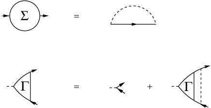
Figure 5: Consistent approximation for the self energy $\Sigma$ and the vertex function ${\bm{\Gamma}}$.

With the results for the spin susceptibility given in I (4.41) - (4.43) we find that only four matrix elements of the potential $V$ are nonzero. They can be expressed in terms of the phase susceptibility, Eq. (37b),

$$V_{12,21}({\bm{k}},{\bm{p}};i\Omega) = \delta_{{\bm{k}}{\bm{p}}}\,\lambda^{2}\,\chi_{\phi\phi}({\bm{k}}-{\bm{q}},i\Omega),$$ (49a)

$$V_{21,21}({\bm{k}},{\bm{p}};i\Omega) = \delta_{{\bm{k}}{\bm{p}}}\,\lambda^{2}\,\chi_{\phi\phi}({\bm{k}}+{\bm{q}},i\Omega),$$ (49b)

$$V_{12,12}({\bm{k}},{\bm{p}};i\Omega) = -\delta_{{\bm{k}}-2{\bm{q}},{\bm{p}}}\,\lambda^{2}\,\chi_{\phi\phi}({\bm{k}}-{\bm{q}},i\Omega),$$

$$V_{21,21}({\bm{k}},{\bm{p}};i\Omega) = -\delta_{{\bm{k}}+2{\bm{q}},{\bm{p}}}\,\lambda^{2}\,\chi_{\phi\phi}({\bm{k}}+{\bm{q}},i\Omega),$$

The development of the transport theory now proceeds analogously to the electron-phonon scattering case, with

$$\lambda^{2}\,\chi_{\phi\phi}({\bm{p}},i\Omega)\equiv V({\bm{p}},i\Omega)$$ (50)

playing the role of the dynamical potential. The chief complications are, (1) the spin structure, which leads to two independent matrix elements, ${\bm{\Gamma}}^{11}$ and ${\bm{\Gamma}}^{12}$ of the vertex function, and (2) the fact that the vector vertex function ${\bm{\Gamma}}_{{\bm{k}}{\bm{p}}}$ depends on the pitch vector ${\bm{q}}$ in addition to ${\bm{k}}$. (${\bm{p}}$ gets eliminated by the Kronecker-$\delta$ constraints in Eqs. (33a) and (49).) In addition, there are two Fermi surfaces, a feature the helimagnetic problem shares with the ferromagnetic one.

As a consequence of the dependence of the vertex function on ${\bm{q}}$, the polarization function, and hence the conductivity, is no longer isotropic. The tensor is still diagonal, but the transverse and longitudinal components, with respect to ${\bm{q}}$, are different,

$$\pi_{ij}(i\Omega)=\delta_{ij}\left[\left(\delta_{i1}+\delta_{i2}\right)\pi_{\text{T}}(i\Omega)+\delta_{i3}\pi_{\text{L}}(i\Omega)\right]$$ (51)

As a consequence of the two Fermi surfaces, the conductivity is the sum of two contributions,

$$\sigma_{\text{L},\text{T}}={\text{Re}}\,\lim_{\omega\to 0}\sigma_{\text{L},\text{T}}(i\Omega\to\omega+i0)=\sigma_{\text{L},\text{T}}^{(1)}+\sigma_{\text{L},\text{T}}^{(2)}.$$ (52)

After calculations that are quite involved, but follow the same reasoning as in the electron-phonon case, one obtains the following expression for the transverse conductivity,

$$\sigma_{\text{T}}^{(i)} = \frac{e^{2}}{2m_{\text{e}}^{2}}\int d\epsilon\,\left(\frac{-\partial f}{\partial\epsilon}\right)\,\frac{1}{V}\sum_{\bm{k}}\delta\left(\omega_{i}({\bm{k}})\right)\,k_{\perp}^{2}\,$$ (53a)

$$\hskip 50.0pt\times\tau_{i}({\bm{k}},\epsilon)\,\Lambda_{i}({\bm{k}},\epsilon).$$

Here $$\tau_{i} \omega_{i} f(\epsilon,T)=1/\exp(\epsilon/T+1) \Lambda_{i} {\bm{\Gamma}}_{{\bm{k}}{\bm{p}}} {\bm{k}}$$ is the quasi-particle relaxation rate given by Eqs. (38), are the resonance frequencies given by Eq. (8), and is the Fermi distribution function. The scalar vertex functions are related to the part of the vector vertex function that is proportional to . As in the electron-phonon case, they obey integral equations which reduce to algebraic equations for the purpose of determining the leading temperature dependence only of the conductivity. We obtain

$$\Lambda_{i}({\bm{k}},\epsilon)=1-\Lambda_{i}({\bm{k}},\epsilon)\,\frac{2\tau_{i}({\bm{k}},\epsilon)}{\left(\xi_{{\bm{k}}+{\bm{q}}}+\xi_{\bm{k}}\right)^{2}}\int du\,\left[n(u)+f(\epsilon+u)\right]\,\frac{1}{V}\sum_{\bm{p}}g_{i}({\bm{k}},{\bm{p}}\,;\epsilon)\,f({\bm{k}},{\bm{p}})\,V^{\prime\prime}({\bm{k}}-{\bm{p}},u)\,\delta(u-\omega_{i}({\bm{p}})),$$ (53b)

where

$$f({\bm{k}},{\bm{p}})=1-\frac{1}{2k_{\perp}^{2}}\,({\bm{k}}-{\bm{p}})_{\perp}^{2}.$$ (53c)

Substituting the solution of Eq. (53b) into Eq. (53a) shows that the conductivity is given in terms of transport relaxation time $\tau_{\text{tr}}$ that is different from the quasi-particle relaxation time $\tau$. Namely,

$$\sigma_{\text{T}}^{(i)}=\frac{e^{2}}{2m_{\text{e}}^{2}}\int d\epsilon\,\left(\frac{-\partial f}{\partial\epsilon}\right)\,\frac{1}{V}\sum_{\bm{k}}\delta\left(\omega_{i}({\bm{k}})\right)\,k_{\perp}^{2}\,\tau_{\text{tr}}^{(i)}({\bm{k}},\epsilon),$$ (54a)

with

$$\frac{1}{2\tau_{\text{tr}}^{(i)}({\bm{k}},\epsilon)} = \frac{-2\pi}{\left(\xi_{{\bm{k}}+{\bm{q}}}+\xi_{\bm{k}}\right)^{2}}\int\frac{du}{\pi}\,\left[n(u)+f(\epsilon+u)\right]\,$$

$$\hskip-20.0pt\times\frac{1}{V}\sum_{\bm{p}}g_{i}({\bm{k}},{\bm{p}})\,V_{2}^{\prime\prime}({\bm{k}}-{\bm{p}},u)\,\delta(u-\omega_{i}({\bm{p}})).$$

Here

$$V_{2}^{\prime\prime}({\bm{k}}-{\bm{p}},u)=\frac{({\bm{k}}-{\bm{p}})_{\perp}^{2}}{2k_{\perp}^{2}}\,V^{\prime\prime}({\bm{k}}-{\bm{p}},u).$$ (54c)

From Eqs. (49) and (37c) it follows that $({\bm{k}}-{\bm{p}})_{\perp}^{2}\sim u\sim T$ in a scaling sense. The leading temperature dependence of the transport relaxation rate $1/\tau_{\text{tr}}$ will therefore carry one higher power of the temperature than the quasi-particle relaxation rate $1/\tau$.

The leading contribution to the longitudinal conductivity is given by Eq. (53a), with $k_{\perp}^{2}$ replaced by $k_{z}^{2}$. Since ${\bm{k}}$ is pinned to the Fermi surface by the $\delta$-function in Eq. (53a), this difference does not change the temperature dependence. The leading temperature dependence of $\sigma_{\text{L}}$ is thus also again given by $\tau_{\text{tr}}$.

Combining these results and observations with the results of Sec. III.2.3 we find the following asymptotic temperature dependence for both the transverse and longitudinal transport relaxation rates due to helimagnons in the ordered phase of a helimagnet with cubic symmetry:

$$1/\tau_{\text{tr}}^{\text{T}}\propto 1/\tau_{\text{tr}}^{\text{L}}\propto\left(\frac{q}{k_{\text{F}}}\right)^{8}\left(\frac{\epsilon_{\text{F}}}{\lambda}\right)^{2}\left[\nu^{4}\left(\frac{T}{T_{q}}\right)^{5/2}\hskip-8.0pt+\left(\frac{T}{T_{q}}\right)^{7/2}\right].$$ (55a)

Here $$\nu T_{q}$$ is the prefactor of the cubic anisotropy in Eq. (41), is defined after Eq. (24), and we have again omitted all numerical prefactors. For both the longitudinal and transverse resistivities, this leads to Eq. (15) with

$$\rho_{5/2}\propto\nu^{4}\,\lambda\left(\frac{q}{k_{\text{F}}}\right)^{8}\,\left(\frac{\epsilon_{\text{F}}}{\lambda}\right)^{2}\,\frac{1}{T_{q}^{5/2}}\ .$$ (55b)

IV Discussion and Conclusion

In summary, we have calculated the effects of the Goldstone mode in the ordered phase of helical magnets, the helimagnon, on the low-temperature behavior of the specific heat, the quasi-particle relaxation rate, and the resistivity. The detailed microscopic calculations given in Sec. III have corroborated the simple physical plausibility arguments given in Sec. II. The helimagnon contribution to the specific heat was found to have a $T^{2}$ temperature dependence, whereas the corresponding contribution from ferromagnetic and antiferromagnetic Goldstone modes goes as $T^{3/2}$ and $T^{3}$, respectively.Kittel (1996) The quasi-particle relaxation rate was found to have a $T^{3/2}$ temperature dependence, which is nonanalytic and stronger than the $T^{2}$ behavior in a Fermi liquid. The resistivity depends on the transport relaxation rate, whose temperature dependence is one power weaker than that of the quasi-particle rate. The asymptotic low-temperature contribution to the resistivity due to electron-helimagnon scattering thus goes as $T^{5/2}$.

We divide our discussion of these results into a semi-quantitative discussion that makes predictions of experimental relevance, and more general theoretical remarks.

IV.1 Predictions for Experiments

The leading low-temperature results given in Sec. III hold for temperatures $T\ll T_{q}$, with $T_{q}$ the temperature scale given after Eq. (24). This can be seen as follows. The helimagnon dispersion relation as given in Eq. (1), or (22b), is valid for wave numbers $k<q$, and crosses over to a different behavior around $k=q$. The energy or temperature scale related to this crossover is thus given by

$$T_{q}\equiv\omega_{0}(k_{z}=q,k_{\perp}=0)=\sqrt{c_{2}}\,\lambda\,q^{2}/k_{\text{F}}^{2}.$$ (56a)

Here we have defined a dimensionless number $$c_{2} c_{z}=c_{2}\,\lambda^{2}q^{2}/k_{\text{F}}^{4} c_{2}=1/36$$ by . Within our weak-coupling model calculation we have , or

$$T_{q}=\lambda\,q^{2}/6k_{\text{F}}^{2},$$ (56b)

which is also the energy of a ferromagnon at $k=q$ within Stoner theory. Estimates for the parameters entering $T_{q}$ that are appropriate for MnSi have been given in I: $q/k_{\text{F}}\approx 0.024$, and $\epsilon_{\text{F}}\approx 23,000\,{\text{K}}$. The value of $\lambda$ is less certain, for reasons explained in I. An upper limit is provided by the Fermi energy, and we use $\lambda/\epsilon_{\text{F}}=1/2$ as a practical upper bound. A likely lower limit is given by $\lambda=520\,{\text{K}}$.Taillefer et al. (1986) Given the large ordered moment in MnSi,Pfleiderer et al. (2001) a value of $\lambda$ that is a sizeable fraction of $\epsilon_{\text{F}}$ is actually more plausible than the latter. For these two extreme choices one obtains $T_{q}\approx 1.1\,{\text{K}}$ and $T_{q}\approx 50\,{\text{mK}}$, respectively. In providing such estimates one should keep in mind that even semi-quantitative estimates are difficult for a system like MnSi that is characterized by a complex Fermi surface and strong interactions.cor It should also be noted that $T_{q}$ gives only the general scale for the crossover; a numerical evaluation of, for instance, the integral that determines the specific heat, Eq. (21), shows clear deviations from the $T^{2}$ behavior already at a temperature of about $0.2T_{q}$. The relevant temperature scale for the interesting helimagnon effects is thus quite low.

To see what the behavior crosses over to at $T\approx T_{q}$, we realize that the term $k_{\perp}^{4}$ in Eq. (22b) is the leading (in a scaling sense) contribution to a term $k^{4}$. For wave numbers $k$ larger than $q$, the dispersion relation is given by $\omega_{0}({\bm{k}})\propto k^{2}$, and $k_{z}$ and $k_{\perp}$ both scale effectively as $T^{1/2}$. For the specific heat at $T>T_{q}$ this implies a helimagnon contribution proportional to $T^{3/2}$. This is the same behavior as in a ferromagnet, since the dispersion relation is effectively ferromagnet-like and the specific heat depends only on the dispersion relation.

A scaling expression for the helimagnon contribution to the specific heat that incorporates both sides of this crossover is

$$C_{V}^{\text{hm}}(T)=q^{3}\,f_{C}(T/T_{q}).$$ (57)

Here $f_{C}$ is a universal scaling function with $f_{C}(x\to 0)=A_{C}\,x^{2}$ and $f_{C}(x\gg 1)=B_{C}\,x^{3/2}$. Here $A_{C}$ is given after Eq. (24), and $B_{C}$ is another universal number.

It is also interesting to compare the helimagnon contribution to the Fermi-liquid one. In the case of the specific heat, this means comparing the first term in Eq. (3) with the second one. In a nearly-free electron model, the coefficient $\gamma$ of the Fermi-liquid term in Eq. (3) is given by $\gamma=k_{\text{F}}^{3}/6\epsilon_{\text{F}}$.Landau and Lifshitz (1980) From Eq. (24), we have $\gamma_{2}=q^{3}A_{C}/T_{q}^{2}$. The helimagnon contribution is equal to the Fermi-liquid one at a temperature

$$T^{*}=\gamma/\gamma_{2}=\frac{1}{36A_{C}}\,\frac{\lambda}{\epsilon_{\text{F}}}\,\frac{k_{\text{F}}}{q}\,T_{q}.$$ (58)

With the value of $k_{\text{F}}/q$ appropriate for MnSi given above, and $\lambda$ a sizeable fraction of $\epsilon_{\text{F}}$, one finds $T^{*}\approx T_{q}$; for smaller values of $\lambda$, $T^{*}$ is correspondingly smaller than $T_{q}$ (which itself has a smaller value). Notice that $T<T^{*}$ does not preclude an observation of the $T^{2}$ helimagnon contribution to the specific heat; it can be extracted by plotting $C/T$ versus $T$.

For the quasi-particle relaxation rate, which can be measured by means of either weak-localization or tunnelling experiments, a similar discussion applies. The results given in Sec. III.2.3 apply for temperatures small compared to $T_{q}$, and at higher temperatures a crossover occurs to a regime that is characterized by an effectively quadratic helimagnon dispersion relation and $k_{z}\sim k_{\perp}\sim T^{1/2}$. Repeating the analysis in Sec. III.2.3 shows that in this regime, $1/\tau({\bm{k}})\propto T$. (We note in passing that this is not the correct result for a ferromagnet, where the Goldstone dispersion relation is effectively the same, but the structure of the equation analogous to Eq. (37a) is different.) This is true irrespective of whether one uses the nearly-free electron energy-momentum relation of Sec. III.2.3 of the cubic one of Sec. III.2.3. This linear temperature dependence is remarkable, although this is not the asymptotic low-temperature contribution, since it deviates so strongly from the quadratic Fermi-liquid result.

A scaling expression that incorporates this limit for both helimagnon contributions to the relaxation rate is

$$\frac{1}{\tau(\bm{k})}=\lambda\,\left(\frac{q}{k_{\text{F}}}\right)^{6}\left(\frac{\epsilon_{\text{F}}}{\lambda}\right)^{2}\left(f_{\tau}^{(5/2)}(T/T_{q})+f_{\tau}^{(3/2)}(T/T_{q})\right),$$ (59)

with $f_{\tau}^{(5/2)}(x\to 0)\propto x^{5/2}$, $f_{\tau}^{(3/2)}(x\to 0)\propto x^{3/2}$, and $f_{\tau}^{(5/2)}(x\gg 1)\propto f_{\tau}^{(3/2)}(x\gg 1)\propto x$.

Again, it is instructive to compare with the corresponding Fermi-liquid result, which is

$$\frac{1}{\tau_{\text{FL}}}=\frac{\pi^{3}}{8}\,\epsilon_{\text{F}}\left(\frac{T}{\epsilon_{\text{F}}}\right)^{2}.$$ (60)

We start with the $T^{5/2}$ term, Eq. (40b), which will be present even in systems with a sizeable lattice anisotropy. It is larger than the Fermi-liquid contribution for temperatures larger than a crossover temperature

$$T^{*}_{2-5/2}=\frac{3\pi^{6}}{2A_{\tau}^{2}}\,\left(\frac{k_{\text{F}}}{q}\right)^{4}\left(\frac{\lambda}{\epsilon_{\text{F}}}\right)^{6}T_{q}.$$ (61)

Due to the high power of the uncertain parameter $\lambda/\epsilon_{\text{F}}$ that enters Eq. (61) it is hard to give even a semi-quantitative estimate. For $\lambda$ a sizeable fraction of $\epsilon_{\text{F}}$ this result suggests that $T^{*}_{2-5/2}$ is substantially larger than $T_{q}$, which means that the $T^{5/2}$ contribution, in the region of its validity, is small compared to the Fermi-liquid term. However, for system with a smaller value of $\lambda/\epsilon_{\text{F}}$ the $T^{5/2}$ contribution may be important. We now turn to the $T^{3/2}$ law that is the asymptotic helimagnon contribution to the relaxation rate for a cubic system. By comparing Eqs. (44) with Eq. (60) one finds that the $T^{3/2}$ law becomes comparable to the Fermi-liquid $T^{2}$ behavior at a temperature

$$T^{*}_{3/2-2}=6\left(\frac{8B\nu^{4}}{\pi^{3}}\right)^{2}\left(\frac{q}{k_{\text{F}}}\right)^{4}\left(\frac{\epsilon_{\text{F}}}{\lambda}\right)^{6}T_{q}$$ (62)

with $B$ from Eq. (44c). The $T^{3/2}$ term is numerically large compared to the Fermi liquid $T^{2}$ contribution for temperatures $T<T^{*}_{3/2-2}$. The numerical value of $T^{*}_{3/2-2}$ depends both on a high power of the parameter $\nu$ in addition to the high power of $\epsilon_{\text{F}}/\lambda$. With $\nu=1$ and $\epsilon_{\text{F}}/\lambda=2$ as above one finds $T^{*}_{3/2-2}\approx 0.025\,T_{q}$. Smaller values of $\lambda$ result in a larger ratio $T^{*}_{3/2-2}/T_{q}$. $T^{*}_{3/2-2}\gtrsim T_{q}$ is necessary for the $T^{3/2}$ term to be numerically large compared to the Fermi-liquid contribution in the entire range of its validity, and for the change from the asymptotic $T^{3/2}$ behavior to the pre-asymptotic $T$ term to occur at a temperature low enough for the helimagnon contribution to be still large compared to the Fermi-liquid contribution. According to the above estimate this is the case for $\lambda\lesssim\epsilon_{\text{F}}/4$.

At this point we need to remember that the helimagnon dispersion relation we have used to calculate the relaxation rate, Eq. (1), is valid only for rotationally invariant systems, while the $T^{3/2}$ behavior is the consequence of an anisotropic electron dispersion relation, Eq. (41). However, since the modification of the helimagnon dispersion is small, namely, on the order of the spin-orbit coupling squared, there still is a large temperature range where the $T^{3/2}$ behavior is realized. To see this, we recall that the spin-orbit coupling $g_{\text{so}}$, which is proportional to $q$, changes Eq. (1) to (see I Eq. (2.23))

$$\omega_{0}({\bm{k}})=\sqrt{c_{z}k_{z}^{2}+c_{\perp}k_{\perp}^{4}+b\,c_{z}q^{2}k_{\perp}^{2}/k_{\text{F}}^{2}}\ ,$$ (63)

where $b$ is a number on the order of unity. If we scale $k_{z}$ and $k_{\perp}$ with appropriate powers of $T$, $c_{z}$, and $c_{\perp}$, such that the main contribution to the integral in Eq. (37a) comes from $k_{z}\approx k_{\perp}\approx 1$, we see that the spin-orbit term in $\omega_{0}$ is unimportant for temperatures

$$T>T_{\text{so}}=b\,\lambda(q/k_{\text{F}})^{4}\propto(q/k_{\text{F}})^{2}T_{q}.$$ (64)

On the other hand, the $T^{3/2}$ term dominates over the $T^{5/2}$ term for temperatures

$$T<T^{*}_{3/2-5/2}=\sqrt{T^{*}_{3/2-2}T^{*}_{2-5/2}}=\frac{8B\nu^{4}}{A_{\tau}}\left(\frac{q}{k_{\text{F}}}\right)^{2}\lambda.$$ (65)

As expected, $T_{\text{so}}$ is small compared to $T^{*}_{3/2-5/2}$ by a factor of $(q/k_{\text{F}})^{2}\propto g_{\text{so}}^{2}$.

Finally, the helimagnon contribution to the resistivity is suppressed compared to the contribution to the quasi-particle scattering rate by a factor of $T/\lambda$. For realistic temperatures one thus expects the Fermi-liquid $T^{2}$ contribution to dominate. This is consistent with the statement in Ref. Pfleiderer et al., 2001 that in the ordered phase of MnSi, the resistivity shows a $T^{2}$ behavior.

IV.2 General remarks

All of our results hinge on the Goldstone mode not being overdamped. In an ultraclean system, a generic band structure actually leads to a weak overdamping of the mode in certain directions in momentum space, which can change the above power laws at very low temperatures.AR_ However, even small amounts of quenched disorder qualitatively weaken the damping, see Sec. IV.E.2 and Ref. 34 in I. The results also hinge on rotational invariance. If the direction of the helix is pinned by the underlying lattice, then the $\sqrt{k_{z}^{2}+k_{\perp}^{4}}$ dispersion relation crosses over to a linear one at asymptotically small wave numbers, and the temperature dependences of the observables will cross over to the same power laws as in the acoustic phonon case. The crossover temperature for this effect to become relevant depends on the strength of the pinning.

For the specific heat we have found that the asymptotic low-temperature dependence is in between the one for ferromagnets and antiferromagnets, respectively, as one might expect from the fact that the helimagnon dispersion relation, Eq. (1), is antiferromagnet-like in the longitudinal direction, and ferromagnet-like in the transverse one. We point out, however, that the Goldstone susceptibility at zero frequency diverges more strongly with vanishing wave vector ${\bm{k}}$ than in the ferromagnetic case. Namely, from Eq. (38b) (or from I Eq. (4.33a)) we see that in the helimagnetic case the static susceptibility diverges as $1/(k_{z}^{2}+{\bm{k}}_{\perp}^{4})$, whereas in a ferromagnet the corresponding behavior is $1/{\bm{k}}^{2}$. One expects this to have dramatic effects for the hydrodynamics, as is the case in certain liquid crystals.Mazenko et al. (1983) This problem will be studied separately.

The transport theory presented in this paper is still at a rather primitive level. We have calculated the resistivity in the simplest possible consistent approximation, which corresponds to a solution of a Boltzmann equation where it is assumed that the bosonic modes remain in thermal equilibrium. Whether this zero-loop approximation yields indeed the leading low-temperature behavior of the resistivity is an open question. In ferromagnets, mode-mode coupling effects (or loops in a field-theoretic language) have been found to induce a square-root frequency dependence in the zero-temperature resistivity.Kirkpatrick and Belitz (2000) Possible similar effects in the helimagnetic case, and the nature of the mode-mode coupling effects at nonzero temperature, remain to be explored. The results of the current calculation, namely, effects of the helimagnons on the conductivity that are weaker than the usual $T^{2}$ Fermi-liquid behavior, are consistent with reports of a $T^{2}$ behavior of the resistivity in the ordered phase of MnSi.Pfleiderer et al. (2001) However, transport in the ordered phase has not been investigated systematically, and the observation of possible mode-mode coupling effects may require measurements at very low temperatures.

The quasi-particle relaxation rate $1/\tau$ has the somewhat surprising property that its temperature dependence depends on the details of the electronic energy-momentum relation $\epsilon_{\bm{k}}$. As was shown in Sec. III.2.3, the generic behavior for an $\epsilon_{\bm{k}}$ consistent with a cubic symmetry is $1/\tau\propto T^{3/2}$, whereas a nearly-free electron model leads to $\tau\propto T^{5/2}$ for generic ${\bm{k}}$. This dependence of asymptotic low-temperature properties on microscopic details is unusual and raises questions about universality. We also note that the prefactor of the leading $T^{3/2}$ behavior depends on the fourth power of the parameter $\nu$ that describes deviations from a nearly-free electron model, see Eq. (44c). In systems where the deviations from nearly-free electron behavior are small, the asymptotic $T^{3/2}$ law could then be confined to extremely low temperatures.

We stress that the current theory deals with the ordered phase of a helimagnet, whereas experimentally much more interesting behavior, namely, a $T^{3/2}$ behavior of the resistivity in violation of Fermi-liquid theory, has been observed in the disordered phase.Pfleiderer et al. (2001) While the current theory has nothing to say about this, the observed remnants of helical order in at least part of the region where the non-Fermi-liquid behavior is observedPfleiderer et al. (2004) makes an understanding of the ordered phase a likely necessary prerequisite for a theoretical treatment of the disordered phase.

Finally, we mention that the results for the quasi-particle relaxation rate and the resistivity presented above hold for clean systems. The presence of quenched disorder can drastically change the transport behavior; this will be investigated in a separate publication.us_

Appendix A Matsubara frequency sums

In this appendix we derive the identity (19). Consider an even function $f(z)=f(-z)$ of one complex argument $z$. Let $f$ have singularities (poles or cuts) on the real axis, but be analytic for ${\text{Im}}\,z>0$. Let $\Omega_{n}=2\pi Tn$ ($n$ integer) be the set of bosonic Matsubara frequencies. Using standard techniques the functional

$$F=T\sum_{n=1}^{\infty}f(i\Omega_{n})$$ (66a)

can be written

$$F=\frac{-i}{2\pi}\int_{-\infty}^{\infty}d\omega\,\nu(\omega)\,f(\omega+i0),$$ (66b)

where

$$\nu(z)=\frac{1}{2}\,\coth\frac{z}{2T}\,-\frac{T}{z}\ .$$ (66c)

The advantage of $\nu(z)$ over the more commonly used Bose distribution function $n(z)$ is that $\nu(z)$ is odd in $z$ and has no pole at $z=0$. On the real axis, $n$ has the property

$$\nu(\omega)=T\,\frac{d}{d\omega}\,\left(\ln\sinh\frac{|\omega|}{2T}-\ln|\omega|\right).$$ (67)

Using this in Eq. (66b), and integrating by parts, yields

$$F=\frac{-T}{\pi}\int_{0}^{\infty}d\omega\,\left[\ln\sinh\frac{|\omega|}{2T}-\ln|\omega|\right]\,\frac{\partial}{\partial\omega}\,{\text{Im}}\,f(\omega+i0).$$ (68)

Only the imaginary part of $f(\omega+i0)$ contributes since the real part is an even function of $\omega$. With $f=\ln\Gamma$ this yields Eq. (19).

References

- Ishikawa et al. (1976) Y. Ishikawa, K. Tajima, D. Bloch, and M. Roth, Solid State Commun. 19, 525 (1976).
- Pfleiderer et al. (1997) C. Pfleiderer, G. J. McMullan, S. R. Julian, and G. G. Lonzarich, Phys. Rev. B 55, 8330 (1997).
- Pfleiderer et al. (2001) C. Pfleiderer, S. R. Julian, and G. G. Lonzarich, Nature 414, 427 (2001).
- Ishikawa and Arai (1984) Y. Ishikawa and M. Arai, J. Phys. Soc. Japan 53, 2726 (1984).
- Pfleiderer et al. (2004) C. Pfleiderer, D. Reznik, L. Pintschovius, H. v. Löhneysen, M. Garst, and A. Rosch, Nature 427, 227 (2004).
- Chaikin and Lubensky (1995) P. Chaikin and T. C. Lubensky, Principles of Condensed Matter Physics (Cambridge University, Cambridge, 1995).
- Belitz et al. (2006) D. Belitz, T. R. Kirkpatrick, and A. Rosch, Phys. Rev. B 73, 054431 (2006).
- (8) S. V. Maleyev, eprint cond-mat/0509406.
- Irkhin and Katsnelson (2000) V. Y. Irkhin and M. I. Katsnelson, Phys. Rev. B 62, 5647 (2000).
- (10) This holds for rotationally invariance systems. The spin-orbit coupling breaks this symmetry, since it couples the electron spins to the underlying lattice. We will discuss the consequences of this (weak) effect in Sec. IV.1.
- (11) We note in passing that the true asymptotic low-temperature contribution to the specific heat is expected to be , since the strong fluctuations that result from the anisotropic helimagnon dispersion relation will not allow for true long-range order; see Ref. 16 in I. We ignore this effect here, as we did in I, as it will become relevant only at extremely long length scales and correspondingly low temperatures.
- Baym and Pethick (1991) G. Baym and C. Pethick, Landau Fermi-Liquid Theory (Wiley, New York, 1991).
- Kittel (1996) C. Kittel, Introduction to Solid State Physics (Wiley, New York, 1996).
- Pines and Nozières (1989) D. Pines and P. Nozières, The Theory of Quantum Liquids (Addison-Wesley, Redwood City, CA, 1989).
- (15) The dynamically screened Coulomb potential represents an infinite resummation. First-order perturbation theory in is therefore sufficient to produce a lifetime. The same result is obtained in second-order perturbation theory with a static potential, in which case the energy conservation inherent in Fermi’s golden rule ensures the quadratic temperature dependence, see Ref. Anderson_1984.
- Abrikosov et al. (1963) A. A. Abrikosov, L. P. Gorkov, and I. E. Dzyaloshinski, Methods of Quantum Field Theory in Statistical Physics (Dover, New York, 1963).
- Fetter and Walecka (1971) A. L. Fetter and J. D. Walecka, Quantum Theory of Many-Particle Systems (McGraw-Hill, New York, 1971).
- Fischer and Rosch (2004) I. Fischer and A. Rosch, Europhys. Lett. 68, 93 (2004).
- (19) In our notation, means “ is proportional to ”, and means “ scales like ”.
- (20) For ferromagnets, the arguments given here do not apply, and we therefore do not discuss this case.
- Lifshitz and Pitaevskii (1981) E. M. Lifshitz and L. P. Pitaevskii, Physical Kinetics (Pergamon, New York, 1981).
- Ziman (1960) J. M. Ziman, Electrons and Phonons (Clarendon Press, Oxford, 1960).
- Ueda (1977) K. Ueda, J. Phys. Soc. Japan 43, 1497 (1977).
- (24) The usual specific heat is defined by this derivative with the volume and the number of particles kept fixed. Here we implicitly keep the volume and chemical potential fixed. For the leading term as these two operations give the same result.
- (25) This remains true if the wave vector dependence of the damping coefficient has a different functional form than the one in I Eq. (4.33c), as long as the mode remains propagating.
- (26) The prefactors of various expressions in I, and Eq. (4.33b) in particular, are incorrect by various factors of 2 or powers of 2. Also, Eq. (4.40) contains typographic errors. A corrected version can be found in cond-mat/0510444.
- Lubensky (1972) T. C. Lubensky, Phys. Rev. A 6, 452 (1972).
- (28) The only stable directions of the pitch vector are or , see Ref. Bak_Jensen_1980. In MnSi, the latter is realized.
- Baym and Kadanoff (1961) G. Baym and L. P. Kadanoff, Phys. Rev. 124, 287 (1961).
- Kadanoff and Baym (1962) L. P. Kadanoff and G. Baym, Quantum Statistical Mechanics (W.A. Benjamin, New York, 1962).
- Taillefer et al. (1986) L. Taillefer, G. Lonzarich, and P. Strange, J. Magn. Magn. Materials 54-57, 957 (1986).
- (32) That MnSi is strongly correlated can be seen from the fact that it has a large magnetic moment of about per formula unit, yet a low transition temperature of about (Ref. Pfleiderer et al., 2004).
- Landau and Lifshitz (1980) L. D. Landau and E. M. Lifshitz, Statistical Physics Part 1 (Butterworth Heinemann, Oxford, 1980).
- (34) A. Rosch, unpublished results.
- Mazenko et al. (1983) G. F. Mazenko, S. Ramaswamy, and J. Toner, Phys. Rev. B 28, 1618 (1983).
- Kirkpatrick and Belitz (2000) T. R. Kirkpatrick and D. Belitz, Phys. Rev. B 62, 952 (2000).
- (37) T.R. Kirkpatrick and D. Belitz, unpublished results.