Percolation on Growing Lattices

Abstract

In order to inverstigate the dependence on lattice size of several observables in percolation, the Hoshen-Kopelman algorithm was modified so that growing lattices could be simulated. By this way, when simulating a lattice of size $L$, lattices of smaller sizes can be simulated in the same run for free, saving computing time.

Here, site percolation in three dimensions was studied. Lattices of up to $L=5000$, with many $L$-steps in between, have been simulated, for occupation probabilities of $p=0.25$, $p=0.3$, $p=p_{c}=0.311608$, and $p=0.35$.

1 Introduction

Percolation is a thoroughly studied model in statistical physics.[1] The algorithm invented by Hoshen and Kopelman in 1976 allows for examing large percolation lattices using Monte Carlo methods,[2] as for simulating a $L^{d}$ lattice only a hyperplane of $L^{d-1}$ sites has to be stored. The normal way to do a simulation using the HK algorithm is to choose an $L$ and an occupation probability $p$, and then walk through the lattice in a linear fashion, calculating interesting observables (like cluster numbers) on the fly or at the end. When one is interested in the dependance of these observables on either $p$ or $L$, one has to repeat these simulations with varying values of these parameters.

In 2000 Newman and Ziff published an algorithm which allows to simulate percolation for all $0\leq p\leq 1$ in one run, making it very easy to study percolation properties in dependance on $p$.[3] Unfortunately, their algorithm lacks a desirable property of the HK algorithm: They need to store the full lattice of $L^{d}$ sites, whereas for HK only memory for $L^{d-1}$ sites is needed.

A slight modification of the HK algorithm allows to simulate percolation for many $1\leq L\leq L_{\mathrm{max}}$ in one run, with only a small performance penalty (depending on the number of intermediate $L$ which are chosen for investigation). The biggest advantage of the HK algorithm, small memory consumption, is preserved. The modified algorithm needs to store three times as much sites as the original one (a constant factor), but this is still $\propto L^{d-1}$, meaning big advantages for low dimensions.

This modified algorithm shall be presented in this paper, along with simulation results for site percolation on the cubic lattice, i. e. $d=3$.

2 Computational method

The traditional HK algorithm works by dividing the $L^{d}$ lattice into $L$ hyperplanes of $L^{d-1}$ sites, then investigating one hyperplane after the other. One advantage of this simple scheme is that it allows for domain decomposition and thus parallelization.[4]

Another approach is to work recursively on growing lattices: first simulate a lattice of size $L^{d}$, then advance to $(L+1)^{d}$ by adding a shell with a thickness of one site onto the old lattice. This way, when simulating an $L_{\mathrm{max}}^{d}$ lattice, all sub-lattices of sizes $L<L_{\mathrm{max}}$ can be investigated; the investigation of intermediate lattices may take some additional time (for counting clusters etc.), but the time spent on generating the full lattice minus time for investigation is the same, because the same number of sites is generated as with the traditional approach.

2.1 A modified Hoshen-Kopelman algorithm

This recursive approach was chosen for this paper. It works as follows: Imagine a cube of size $L^{3}$. It has six faces, labelled A, B, C, X, Y, Z (cf. fig. 1). In order to increase the size $L$ of the cube by one, three new faces A’, B’, C’ with a thickness of one are slapped onto the old faces A, B, C; additionally, edges AB, BC, and CA, and a corner ABC are added, forming a full $(L+1)^{3}$ cube.

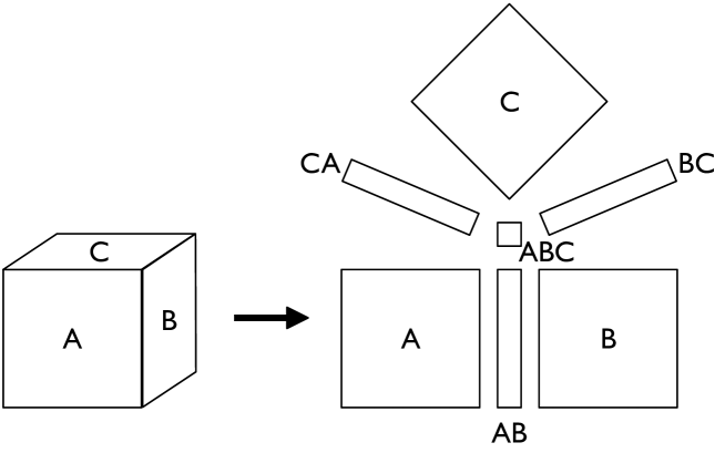
Figure 1: Decomposition of the surface of the cubic lattice. Rear faces X, Y, and Z are not shown. Due to the Hoshen-Kopelman algorithm, in $d$ dimensions, only a $d-1$ hyperplane needs to be stored, here for the growing cube only its surface. When going from an $L$-cube to an $L+1$-cube, the surface grows. As edges and corners have to be treated specially, they are stored separately. For a $L\times L\times L$ cube, the faces (A, B, C) are $L-1\times L-1$, the edges (AB, BC, CA) $L-1\times 1$, and the corner (ABC) is $1\times 1$.

Using the HK algorithm (both the original and the modified version), each newly generated site has $d$ old neighbors. For $d=3$, we have top, left, and back neighbors. For the sake of simplicity, we assume here that top and left neighbors are within a new face A’ (resp. B’, C’), while back neighbors are in the old face A. Due to geometry, site numbering is shifted by one: the site A’$(i>0,j>0)$ has a back neighbor of A$(i-1,j-1)$. A’$(0,j>0)$ has a back neighbor CA$(j-1)$, A’$(i>0,0)$ has a back neighbor AB$(i-1)$, and A’$(0,0)$ has ABC. Thus edges and the corner need to be treated specially (cf. fig. 2 for more clarity).

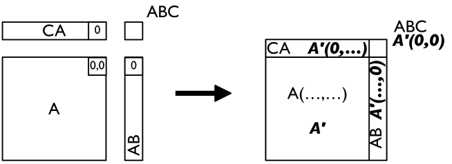
Figure 2: When growing the cube from $L$ to $L+1$, the surface which needs to be stored for the Hoshen-Kopelman algorithm, needs to grow, too. The faces of the cube, here A, grow from $L-1\times L-1$ (A, plain font in figure) to $L\times L$ (A’, bold italic in figure). For the largest part of A’, A’$(i>0,j>0)$, the back neighbors are sites of A, but for the inner rim of A’, A’$(i=0,j>0)$ resp. A’$(i>0,j=0)$, the back neighbors are CA resp. AB. For A’$(0,0)$, it is ABC.

The site A’$(i,j)$ has the left neighbor A’$(i+1,j)$ and the top neighbor A’$(i,j+1)$, when we start working inwards from A’$(L,L)$. This way, we do not need to store A and A’, but can overwrite A with the values of A’. The same trick is used in the original HK algorithm for storing only one hyperplane instead of two.

This way we need three faces of size $(L-1)^{2}$, three edges of $L-1$ and one corner of size 1, for a total of $3L^{2}-3L+1$ sites, in order to simulate a system of size $L^{3}$. For the traditional approach, we need $L^{2}$ sites, meaning one third, a fixed factor. But we need an additional label array for both methods, so that memory consumption does not differ drastically.

As the new approach has about the same speed and only moderately higher memory consumption than the traditional one, it is a viable alternative.

One important thing to keep in mind is that for a single run, results for $L_{1}$ and $L_{2}>L_{1}$ are not statistically independent, e. g. results for $L$ and $L+1$ are naturally highly correlated. This problem can be alleviated by averaging over many runs with different random numbers, because results for different random numbers are suitably statistically independent, as long as the used random number generator has a sufficiently high quality.

2.2 Fully periodic boundary conditions

For small lattices, open boundaries would mean a strong distortion of results, in the most cases proportional to $1/L$ (surface divided by volume). In order to get rid of these influences, it is necessary to use periodic boundary conditions, i. e. sites on an open border are connected to corresponding sites on the opposite border.

This is also possible for the modified HK algorithm. It is necessary to store not only the front faces A, B, C, but also the rear faces X, Y, Z. When we choose to obtain observables for an intermediate lattice size $L$, we connect sites on A to Z, on B to Y, and on C to X.

When during periodicization a cluster on one face connects to the same cluster on the opposite face, that cluster spans the whole systems and wraps around, and thus can be identified as the infinite cluster. When such a cluster is detected, the system percolates. It is possible that more than one such cluster forms; the number of different spanning clusters is counted as $n_{\infty}$.

As the label array is modified by periodicization, we need to save a copy first, because we need the original array to continue the simulation for larger $L$ afterwards. After the periodicization, the modified label array contains all cluster properties; these can be easily extracted and written out. The modified array can be discarded afterwards.

Using this method, it is possible to use fully periodic boundary conditions for intermediate $L$, although the lattice grows afterwards. Periodic b. c. mean a performance penalty and a doubling of memory consumption (as six faces instead of three need to be stored). But the same is also true of the traditional HK algorithm for periodic b. c., were two instead of one hyperplane need to be stored, still giving a factor of three in memory consumption.

2.3 Recycling of labels

When simulating large lattices, the label array is filled with labels, to which sites in the lattice point. Due to the way with which the HK algorithm (both original and modified version) works, lots of these labels are indirect ones, which point to other labels. Other labels correspond to clusters that are hidden in the bulk of the lattice and no longer touch a surface. It is possible to get rid of these labels and thus free up precious space by using a method known as Nakinishi recycling.[5]

In order to support fully periodic b. c., for each recycling all labels represented in A, B, C, X, Y, Z, AB, BC, CA, ABC, have to be taken into account. The method is fully analogous to that used for the traditional HK algorithm.

3 Results

All simulations were done using the R$(471,1586,6988,9689)$ pseudo-random number generator.[6] The value of $p_{c}$ is not known exactly for site percolation on the cubic lattice. For this paper it was chosen as $p_{c}=0.311608$.[7] Simulations were done for $p=0.25,0.3,p_{c},0.35$, in order to investigate behavior below, at, and above the critical threshold. For each value of $p$, 1000 runs with different random numbers were made and used for averaging. Total required CPU time was 10000 hours on 2.2 GHz Opteron processors.

3.1 Cluster size distribution

For the number $N_{s}$ of clusters of size $s$ in a lattice, we expect a distribution $N_{s}\propto s^{-\tau}$ right at $p_{c}$. To make analysis easier, we look at $n_{s}$, the number of clusters with at least $s$ sites:

$$n_{s}=\sum^{\infty}_{s^{\prime}=s}N_{s^{\prime}}\simeq ks^{-\tau+1}$$ (1)

In a log-log-plot, we would expect a straight line with slope $-\tau+1$. Deviations from the power law would be hard to detect due to the logarithmic scale, thus we plot $s^{\tau-1}n_{s}$ linearly on the $y$-axis. By varying $\tau$ until a flat plateau forms, we can estimate $\tau=2.189(1)$. We can clearly see in fig. 3 the deviation for small $s$, which are the same for different $L$, and for large $s$, which differ for various $L$, as these are caused by the finite system size.

Figure 3: Cluster size distribution $n_{s}$ for $L=50$ ($\Box$), $L=500$ ($\times$), and $L=5000$ ($+$). By plotting $n_{s}s^{\tau-1}L^{-3}$, all points should fall on the same line. For small $s$, we can see corrections to scaling, for large $s$ the effects of the finite system size, even though the boundary conditions are fully periodic. For larger $L$, the finite size effects occur for larger $s$.

For $p<p_{c}$, $n_{s}$ drops off sharply for small $s$, with $s$ slowly growing for growing $L$ (not plotted). The same is true for $p>p_{c}$, but there does an additional infinite cluster form (not plotted, too).

3.2 Number of infinite clusters

An infinite cluster is a cluster that spans the whole system. When using periodic b. c., this cluster needs to wrap around, i. e. span the whole system and then periodically connect to itself.

According to theory, for $p<p_{c}$ no infinite cluster is expected, for $p=p_{c}$ about one with fractal properties, and for $p>p_{c}$ one with bulk properties. The critical threshold $p_{c}$ is well-defined only for infinite lattices, where the number of infinite clusters (when these clusters are really infinite) $n_{\infty}$ is exactly zero below $p_{c}$ and exactly one above $p_{c}$. For finite lattices, it is reasonable to define $p_{c}$ so that the average number of infinite clusters is $1/2$, i. e. a spanning cluster forms as often as it does not. Below $p_{c}$, $n_{\infty}$ drops sharply to zero, above $p_{c}$ it goes up sharply to one. $p_{c}$ depends on the lattice size.

For simulations at $p_{c}$, here a value of $p=0.311608$ was chosen. As can be seen form fig. 4, this value is slightly too small, but still very near at the true value for $p_{c}$. An interesting behavior for $n_{\infty}$ results: $n_{\infty}\propto(\log L)^{-3/4}$.

Figure 4: Number $n_{\infty}$ of infinite clusters, at $p=0.311608\simeq p_{c}$, averaged over 1000 runs, depending on lattice size $L$. Right at $p_{c}$ we expect $n_{\infty}=1/2$, i. e. a spanning cluster forms as often as it does not. As here $n_{\infty}<1/2$, the value $p=0.311608$ chosen for this paper is slightly to small; due to finite size effects, sufficiently large lattices have to be simulated in order to see this, even when using periodic b. c. For the number of infinite clusters we get $n_{\infty}=0.3(\log_{10}L)^{-3/4}$.

For $p>p_{c}$, $n_{\infty}$ is expected to be exactly equal one. This is true for lattice sizes $L>50$, but for smaller lattices sizes, an interesting behavior is visible (cf. fig. 5): for very small lattices, less than one infinite cluster forms on average, for slightly larger lattices, sometimes more than one such cluster forms.

Figure 5: Number $n_{\infty}$ of infinite clusters (i. e. that wrap around the system) for $p=0.35$, depending on lattice size. Theory predicts that only one such cluster forms. However, for small lattice sizes a complex finite size behavior can be seen: for $L<17$, less than one infinite cluster forms on average, for $L>17$ more than one cluster forms, with a maximum at $L=22$, afterwards $n_{\infty}$ drops to $1$ exponentially. The solid line corresponds to $1+e^{-0.29(L-16.2)}$. For this plot, $10^{7}$ runs of up to $L=50$ have been averaged.

For $p<p_{c}$, no infinite cluster forms for even small $L$. Only for very small $L$, sometimes an infinite cluster appears. For larger $p$ this $L$ becomes larger (not plotted).

3.3 Size of largest cluster

As mentioned above, the infinite cluster has fractal properties at $p=p_{c}$, meaning that it grows $\propto L^{D}$, with $D$ a non-integer value. From fig. 6 we can extract a value of $D=2.52(1)$.

Figure 6: Size $s_{\mathrm{max}}$ of the largest cluster (which is the infinite cluster, if it forms), at $p=p_{c}$, scaled by $L^{D}$, depending on simulated lattice size. The cluster grows $\propto L^{D}$, with a fractal dimension of $D=2.52(1)$. Thus, by scaling, we get a straight line (the line visible in the plot serves as guide to the eye). For very small lattice sizes $L$, corrections to scaling can be seen.

For $p>p_{c}$, the infinite cluster obtains bulk properties, i. e. it grows $\propto L^{D}$ with $D=3$; it has no longer fractal properties (not plotted).

For $p<p_{c}$, we expect the largest cluster (which does not span the whole lattice) to grow $\propto\log L$, cf. fig. 7. This is true for $p=0.25$ and $p=0.3$ (not plotted), only slope and intercept are different. From fig. 7 another important effect can be seen: although it seems natural to determine the largest cluster $s_{\mathrm{max}}$ by taking the largest cluster of all independent runs, this would mean that no averaging happens, and thus the values of $s_{\mathrm{max}}$ are not statistically independent for different $L$: a large cluster in one single run would dominate the results. Thus, even here averaging is necessary to obtain meaningful results.

Figure 7: Size $s_{\mathrm{max}}$ of the largest cluster, at p=0.25, depending on simulated lattice size. $+$ are for $s_{\mathrm{max}}$ averaged over 1000 runs, $\times$ for the maximal $s_{\mathrm{max}}$ of 1000 runs, which has stronger fluctuations (as the maximum is determined by single clusters; in fact, as no averaging is done, the results for $L$ and $L+1$ are not statistically independent). The solid line corresponds to $300\log_{10}(L)-355$, the dashed line to $320\log_{10}(L)-180$. Thus, for $p<p_{c}$, the largest cluster grows $\propto\log(L)$.

4 Summary

It is possible to modify the Hoshen-Kopelman algorithm in order to obtain not only results for a $L_{\mathrm{max}}^{d}$ lattice in one simulation run, but also results for intermediate $L$ with $L<L_{\mathrm{max}}$. Compared to the original HK algorithm, there is a small performance penalty and a higher memory consumption (a constant factor of $d$ for storing the lattices sites). The modified algorithm is very useful in order to study the dependance of percolation properties on the lattice size.

In this paper, the new algorithm was used for site percolation on the cubic lattice, i. e. $d=3$, lattice sizes up to $5000^{3}$, and occupation probabilities below, at, and above $p_{c}$. Results are presented for cluster size distribution, number of infinite clusters, and size of the largest cluster.

5 Outlook

A natural next step would be to move away from three dimensions and to adapt the algorithm to different $d$. Adapting it to $d=2$ is easy, while $d>3$ is not easy, but still straightforward.

Parallelization by using domain decomposition is apparently very hard, as the size of the domains would be changing. This would only be necessary in order to simulate huge lattices, where the $L$-dependence might not be very interesting. As several runs always need to be averaged, in order to obtain statistically independent data, replication is always a viable parallelization strategy.

References

- [1] D. Stauffer, A. Aharony, Introduction to Percolation Theory, (Taylor & Francis, London, 1994).
- [2] J. Hoshen, R. Kopelman, Phys. Rev. B 14, 3438 (1976).
- [3] M. E. J. Newman, R. M. Ziff, Phys. Rev. Lett. 85, 4104 (2000); see also J. E. de Freitas, L. S. Lucena, Int. J. Mod. Phys. C 11, 1581 (2000).
- [4] D. Tiggemann, Int. J. Mod. Phys. C 12, 871 (2001).
- [5] H. Nakanishi, H. E. Stanley, Phys. Rev. B 22, 2466 (1980).
- [6] R. M. Ziff, Comput. in Phys. 12, 385 (1998).
- [7] C. D. Lorenz, R. M. Ziff, J. Phys. A 31, 8147 (1998); H. G. Ballesteros et al., J. Phys. A 32, 1 (1999).