Solubility in Compressible Polymers: Beyond the Regular Solution Theory

Abstract

The age-old idea of ”like dissolves like” requires a notion of ”likeness” that is hard to quantify for polymers. We revisit the concepts of pure component cohesive energy density $c^{\text{P}}$ and mutual cohesive energy density $c_{12}$ so that they can be extended to polymers. We recognize the inherent limitations of $c_{12}$ due to its very definition, which is based on the assumption of no volume of mixing (true for incompressible systems), one of the assumptions in the random mixing approximation (RMA); no such limitations are present in the identification of $c^{\text{P}}.$ We point out that the other severe restriction on $c_{12}$ is the use of pure components in its definition because of which $c_{12}$ is not merely controlled by mutual interactions. Another quantity $c_{12}^{\text{SRS}}$ as a measure of mutual cohesive energy density that does not suffer from the above limitations of $c_{12}$ is introduced. It reduces to $c_{12}$ in the RMA limit. We are able to express $c_{12}^{\text{SRS}}$ in terms of $c_{12}$ and pure component $c^{\text{P}}$’s. We also revisit the concept of the internal pressure and its relationship with the conventional and the newly defined cohesive energy densities. In order to investigate volume of mixing effects, we introduce two different mixing processes in which volume of mixing remains zero. We then carry out a comprehensive reanalysis of various quantities using a recently developed recursive lattice theory that has been tested earlier and has been found to be more accurate than the conventional regular solution theory such as the Flory-Huggins theory for polymers. In the RMA limit, our recursive theory reduces to the Flory-Huggins theory or its extension for a compressible blend. Thus, it supersedes the Flory-Huggins theory. Consequently, the conclusions based on our theory are more reliable and should prove useful.

I Introduction

I.1 Pure Component and Athermal Reference State

Understanding the solubility of a polymer in a solvent is a technologically important problem. It is well documented that ”like dissolves like” but it is almost impossible to quantify the notion of ”likeness” of materials. The understanding of solubility requires a basic understanding of ”likeness” that is lacking at present. Solubility parameters in all their incarnations are attempts to quantify this simple notion. There are several ways one can proceed to understand solubility by considering various thermodynamic quantities, not all of which are equivalent. However, almost all these current approaches are based on our thermodynamic understanding of mixtures at the level of the regular solution theory (RST) vanLaar ; Hildebrand1916 ; Hildebrand .

In practice, one usually introduces the Hildebrand solubility parameter

$$\delta=\sqrt{c^{\text{P}}}$$

for a pure component in terms of $c^{\text{P}},$ the latter being the cohesive energy density of the pure (P) component and is normally reported at its boiling temperature. In this work, we will take this definition to be operational at any temperature, thus treating $\delta$ as a thermodynamic quantity, and not just a parameter. Then its value at the boiling point will be the customarily quoted solubility parameter. The cohesive energy is related to the interaction energy $\mathcal{E}_{\text{int}}$ obtained by subtracting the energy $\mathcal{E}_{\text{ath}}$ of the hypothetical athermal state of the pure component, the state in which the self-interactions (both interparticle and intraparticle) are absent, from the total energy $\mathcal{E}$:

$$\mathcal{E}_{\text{int}}\ \equiv\mathcal{E-E}_{\text{ath}}.$$ (1)

The athermal state is usually taken to be at the same temperature $T$ and the volume $V$ as the system itself. In almost all cases of interest, $\mathcal{E}_{\text{ath}}$ is nothing but the kinetic energy and depends only on $T$ but not on $V.$ Thus, $\mathcal{E}_{\text{int}}$ depends directly on the strength of the self-interaction, the only interaction present in a pure component and vanishes as self-interactions disappear, since $\mathcal{E}\rightarrow\mathcal{E}_{\text{ath}}$ as this happens. Thus, $\mathcal{E}_{\text{int}}$ can be used to estimate the strength of the self-interaction. One can also take the hypothetical state to be at the same $T$ and the pressure $P$. In this case, there would in principle be a difference in the volume $V$ of the pure component and $V_{\text{ath}}$ of the hypothetical state, but this difference will not change $\mathcal{E}_{\text{int}}$ in (1). The hypothetical state is approximated in practice by the vapor phase at the boiling point in which the particles are assumed to be so far apart that their mutual interactions can be neglected. However, to be precise, it should be the vapor phase at zero pressure so that the volume is infinitely large to make the particle separation also infinitely large to ensure that they are non-interacting. This causes problems for polymers Choi . Our choice of the athermal state in (1) to define $\mathcal{E}_{\text{int}}$ overcomes these problems altogether. By definition,

$$c^{\text{P}}\equiv-\mathcal{E}_{\text{int}}/V$$ (2)

is the negative of the interaction energy density (per unit volume $V)$ of the system at a given temperature $T.$ (At the boiling point, $V$ is taken to be the volume of the liquid). The negative sign is to ensure $c^{\text{P}}>0$ since usually $\mathcal{E}_{\text{int}}$ is negative to give cohesion. Because of its dimensions, $c^{\text{P}}$ is also known as the cohesive pressure. In this form, $c^{\text{P}}$ is a thermodynamic quantity and represents the thermodynamically averaged (potential) energy per unit volume of the pure component. Thus, $c^{\text{P}}$ can be calculated even for macromolecules like polymers, which is of central interest in this work or for polar solvents. It is a macroscopic, i.e. a thermodynamic quantity characterizing microscopic interparticle interactions in a pure component. This is important as it is well known that $\delta$ cannot be measured directly as most polymers cannot be vaporized without decomposing Du . Thus, theoretical means are needed to evaluate $\delta,$ which is our goal in this work.

It should be noted from the above definition that $c^{\text{P}}$ contains the contributions from all kinds of forces (van der Waals, dipolar, and hydrogen bonding forces) in the system Hansen . In this work, we are only interested in the weak van der Waals interactions for simplicity, even though the investigation can be easily extended to include other interactions. It should also be noted that the definition (2) does not suffer from any inherent approximation, and can be used to calculate $c^{\text{P}}$ in any theory or by experimental measurements. As we will see, this is not true of the mutual cohesive density definition, which is introduced below.

I.2 Mixture and Self-interacting Reference State

As it stands, the pure component quantity $c^{\text{P}}$ is oblivious to what may happen in a mixture formed with another component. Despite this, $c^{\text{P}}$ or $\delta$ is customarily interpreted as a rough measure of a solvent’s ability to dissolve a solute (”like dissolves like”). This interpretation of the solubility parameter is supposed to be reliable only for non-polar solvents formed of small molecules, and one usually refrains from using it for polar solvents such as esters, ketones, alcohol, etc. Our interest is to investigate this quantity for macromolecules here, and its significance for the solubility in a mixture. According to the famous Scatchard-Hildebrand relation Hildebrand , the energy of mixing $\Delta E_{\text{M}}$ per unit volume for a binary mixture of two components $1$ and $2$ must always be non-negative since it is given by

$$\Delta E_{\text{M}}=(\delta_{1}-\delta_{2})^{2}\varphi_{1}\varphi_{2},\ \ \ \ (\varphi_{1}+\varphi_{2}\equiv 1),$$ (3)

where $\varphi_{i}$ are the volume fractions of the two components $i$, and $\delta_{1}$ and $\delta_{2}$ are their solubility parameters. It is implicitly assumed here that the volume of mixing $\Delta V_{\text{M}}=0$. Thus, this expression does not contain the contribution from a non-zero volume of mixing. We will be interested in investigating this additional contribution in this work. Later, we will discover that (3) can only be justified [see (41) below], if we take

$$\varphi_{i}\equiv\phi_{\text{m}i}/\phi_{\text{m}},\ \ \ \ \ (\phi_{\text{m}}\equiv\phi_{\text{m}1}+\phi_{\text{m}2})$$ (4)

as representing the monomer density ratios, or monomer fractions; see below for precise definition. Only in the RST can we identify $\varphi_{i}$ with the volume fraction of the $i$th component. The significance of (3) is that the behavior of the mixture is completely determined by the pure component properties and provides a justification for ”like dissolves like”. This must be a gross approximation even for non-polar systems and cannot be true in general since the energy of mixing can be negative in many cases, as shown elsewhere Gujrati2003 , and as we will also see here later; see, for example, Fig. 16. What we discover is that $\Delta E_{\text{M}}$ can be negative even if $\Delta V_{\text{M}}=0$. Thus, zero volume of mixing is not sufficient for the validity of (3).

For the mixture, we need to introduce a thermodynamic or macroscopic quantity $c_{12}$ characterizing the mutual interaction between the two components; this quantity should be determined by the microscopic interaction between the two components. Therefore, the introduction of $c_{12}$ will, in principle, require comparing the mixture with a hypothetical mixture in which the two components have no mutual interactions similar to the way the pure component (having self-interaction) was compared with the athermal state above (in which the self-interaction was absent) for the introduction of $c^{\text{P}}.$ The hypothetical state of the mixture should not be confused with the athermal state of the mixture; the latter will require even the self interaction of the two components to be absent. The new hypothetical state will play an important role in our investigation and will be called self-interacting reference state (SRS). The mutual interaction energy in the binary mixture is obtained by subtracting the energy of SRS from that of the mixture:

$$\mathcal{E}_{\text{int}}^{(\text{M})}\ \equiv\mathcal{E-E}_{\text{SRS}};$$ (5)

compare with (1). Just as before, SRS can be taken at the same $T$ and $V,$ or $T$ and $P$ as the mixture. This allows us to separate out the two contributions, one due to the presence of mutual interactions at the same volume $V_{\text{SRS}}=V$ of SRS, and the second contribution due to merely a change in the volume from $V_{\text{SRS}}$ to $V;$ this was not the case with $\mathcal{E}_{\text{int}}$ above. Each contribution of $\mathcal{E}_{\text{int}}^{(\text{M})}$ vanishes as mutual interactions disappear, since $\mathcal{E}\rightarrow\mathcal{E}_{\text{SRS}},$ and $V_{\text{SRS}}\rightarrow V$ as this happens. If $\mathcal{E}_{\text{int}}^{(\text{M})}$ is used to introduce a mutual cohesive energy density (to be denoted later by $c_{12}^{\text{SRS}}$), then such a density would most certainly vanish with vanishing mutual interaction strength. However, this is not the conventional approach adopted in the literature when introducing $c_{12}$. Rather, one considers the energy of mixing. We will compare the two approaches in this work. Whether the conventionally defined $c_{12}$ vanishes with the mutual interactions remains to be verified. In addition, whether it is related to the pure component self interaction cohesive energy densities $c_{11}^{\text{P}}$ and $c_{22}^{\text{P}}$ in a trivial fashion such as (10), see below, needs to be investigated. As we will see, this will require further assumptions even within RST to which we now turn.

I.3 Regular Solution Theory (RST)

The customary approach to introduce $c_{12}$ is to follow the classical approach developed by van Laar, and Hildebrand vanLaar ; Hildebrand1916 ; Hildebrand , which is based on RST, a theory that can be developed consistently only on a lattice. The theory describes an incompressible lattice model or a compressible model in which the volume of mixing $\Delta V_{\text{M}}$ is zero. The lattice model is introduced as follows. One usually takes a homogeneous lattice of coordination number $q$ and containing $N$ sites. The volume of the lattice is $Nv_{0}$ where $v_{0}$ is the lattice cell volume. We place on this lattice the polymer (component $1$) and the solvent (component $2$) molecules in such a way that the connectivity of the molecules are kept intact. It should be stressed that the solvent molecules themselves may be polymeric in nature. In addition, the excluded volume interactions are enforced by requiring that no site can be occupied by more than one monomer at a time. The monomer densities of the two components $\phi_{\text{m}i}$ ($i=1,2)$ are the densities of sites occupied by the $i$th component. Two monomers belonging to components $i$ and $j,$ respectively, interact with an energy $e_{ij}=$ $e_{ji}$ only when they are nearest-neighbor. (This nearest-neighbor restriction can be easily relaxed, but we will not do that here for simplicity.) The interaction between the polymer and the solvent is then characterized by a single excess energy parameter $\varepsilon\equiv\varepsilon_{12}$ defined in general by the combination

$$\varepsilon_{ij}\equiv e_{ij}-(1/2)(e_{ii}+e_{jj}).$$ (6)

The origin of this combination is the fixed lattice connectivity as shown elsewhere Gujrati2000 . For an incompressible binary mixture for which

$$\phi_{\text{m}1}+\phi_{\text{m}2}=1,$$

the excess energy $\varepsilon$ is sufficient for a complete thermodynamic description on a lattice Gujrati2000 .

On the other hand, a compressible lattice model of the mixture, which requires introducing voids as a separate component ($i=0$), will usually require two additional excess energy parameters $\varepsilon_{01},$ and $\varepsilon_{02}$ Gujrati1998 . In the following, we will implicitly assume that a void occupies a site of the lattice and has it occupies a volume $v_{0}.$ In our picture, a pure component is a pseudo-binary mixture ($i=0,1$ or $i=0,2),$ while a compressible binary mixture is a pseudo-tertiary mixture ($i=0,1,2).$

Since voids do not interact with themselves or with any other component, we must set

$$e_{00}=e_{0i}=0,$$

so that the corresponding excess energy

$$\varepsilon_{0i}=-(1/2)e_{ii},$$ (7)

see (6), and is normally positive since $e_{ii}$ is usually negative.

Two of the three conditions for RST to be operative are

(i) Isometric Mixing: $\Delta V_{\text{M}}$ $\equiv 0$, and

(ii) Symmetric Mixture: The two components must be of the same size and have the same interaction ($e_{11}\equiv e_{22}$). This is a restatement of ”like dissolves like.”

The condition $\Delta V_{\text{M}}=0$ for isometric mixing is always satisfied in an incompressible system. For a compressible system, $\Delta V_{\text{M}}$ need not be zero, and one can have either an isometric or a non-isometric mixing depending on the conditions.

I.3.1 Random Mixing Approximation (RMA)

The third condition for RST to be valid is the fulfillment of the

iii) RMA Limit: The interaction energy $\varepsilon_{ij}$ be extremely weak ($\varepsilon_{ij}\rightarrow 0$), and the coordination number $q$ of the lattice extremely large ($q\rightarrow\infty$) simultaneously so that the product

$$q\varepsilon_{ij}\text{ remains fixed and finite, as }\varepsilon_{ij}\rightarrow 0,\text{ and }q\rightarrow\infty.$$

Indeed, if one introduces the dimensionless Flory-Huggins chi parameter $\chi_{ij}\equiv\beta q\varepsilon_{ij},$ where $\beta\equiv 1/k_{\text{B}}T,$ $T$ being the temperature in the Kelvin scale, then one can also think of keeping $\chi_{ij}$ fixed and finite, instead of $q\varepsilon_{ij},$ under the simultaneous limit

$$\chi_{ij}\equiv\beta q\varepsilon_{ij}\text{ fixed and finite, as }\beta\varepsilon_{ij}\rightarrow 0,\text{ and }q\rightarrow\infty.$$ (8)

It is quite useful to think of RST in terms of these limits as both $\beta\varepsilon_{ij}$ and $q$ are dimensionless. The above simultaneous limit gives rise to what is usually known as the random mixing approximation (RMA), and has been discussed in detail in a recent review article Gujrati2003 in the context of polymer mixtures. For an incompressible system, we need to keep only a single chi parameter $\chi\equiv\beta q\varepsilon$ fixed and finite in the limit. For a compressible system, one must also simultaneously keep the two additional chi parameters related to $\varepsilon_{01}$ and $\varepsilon_{02},$ and $\beta Pv_{0}$ fixed and finite, where $P$ is the pressure Gujrati1998 ; Gujrati2003 .

The RMA limit can be applied even to a pure component (for which the first two conditions are meaningless). It can also be applied when mixing is not isometric Note1 or when the mixture is not symmetric. Therefore, RST is equivalent to the isometric RMA. In the unusual case $\chi=0,$ ($q\rightarrow\infty),$ the resulting isometric theory is known as the ideal solution theory, which will not be considered here as we are interested in the case $\chi\neq 0.$

I.3.2 London-Berthelot and Scatchard-Hildebrand Conjectures

The energy of mixing $\Delta E_{\text{M}}$ per unit volume is the central quantity for solubility considerations, and can be used to introduce an effective ”energetic” chi Gujrati1998 ; Gujrati2003 as follows:

$$\chi_{\text{eff}}^{\text{E}}\equiv\beta\Delta E_{\text{M}}v_{0}/\phi_{\text{m}1}\phi_{\text{m}2},$$ (9)

which is a measure of the Flory-Huggins $\chi(\equiv\chi_{12})$ parameter or the excess energy $\varepsilon(\equiv\varepsilon_{12})$; the latter is directly related to the mutual interaction energy $e_{12},$ see (6), which explains the usefulness of $\Delta E_{\text{M}}$ for solubility considerations. One of the important consequences of the application of RST is the Scatchard-Hildebrand conjecture Hildebrand , according to which the energy of mixing is given by a non-negative form (3). This is known to be violated; see Gujrati2003 , and below. One of the reasons for its failure could be the much abused London-Berthelot conjecture

$$c_{12}=\sqrt{c_{11}^{\text{P}}c_{22}^{\text{P}}}\equiv\delta_{1}\delta_{2},$$ (10)

relating the mutual cohesive energy density $c_{12}$ with the pure component cohesive energy densities $c_{11}^{\text{P}},$ $c_{22}^{\text{P}},$ and used in the derivation of (3). In contrast, the London conjecture

$$e_{12}=-\sqrt{(-e_{11})(-e_{22})}$$ (11)

deals directly with the microscopic interaction energies, and is expected to hold for non-polar systems; see also Israelachvili for an illuminating derivation and discussion. In the isometric RMA limit, the two conjectures become the same in that (11) implies (10). In general, they are two independent conjectures. As we will demonstrate here, (11) does not imply (10) once we go beyond the RMA limit. We will also see that the non-negativity of the form (3) is violated even for isometric mixing.

Association of one component, such as through hydrogen bonding, usually makes $e_{12}^{2}<\left|e_{11}\right|\left|e_{22}\right|.$ On the other hand, complexing results in the opposite inequality $e_{12}^{2}>\left|e_{11}\right|\left|e_{22}\right|.$ It is most likely that the binary interaction between monomers of two distinct species will deviate from the London conjecture (11) to some degree. Thus, some restrictions have to be put on the possible relationship between these energy parameters for our numerical calculations. We have decided to consider only those parameters that satisfy the London conjecture (11) in this work for physical systems.

I.3.3 Deviation from London-Berthelot Conjecture

The deviation from the London-Berthelot conjecture (10) is usually expressed in terms of a binary quantity $l_{12}$ defined via

$$c_{12}=\sqrt{c_{11}^{\text{P}}c_{22}^{\text{P}}}(1-l_{12}),$$ (12)

and it is usually believed that the magnitude of $\ l_{12}\$is very small:

$$\left|l_{12}\right|<<1.$$ (13)

It is possible that $l_{12}$ vanishes at isolated points, so that the London-Berthelot conjecture becomes satisfied. This does not mean that the system obeys RST there. As we will demonstrate here, we usually obtain a non-zero $l_{12}$, thus implying a failure of the London-Berthelot conjecture (10), even if the London conjecture (11) is taken to be operative. Another root for the failure of (10) under this assumption could be non-isometric mixing. A third cause for the failure could be the corrections to the RMA limit, since a real mixture is not going to truly follow RST. To separate the effects of the three causes, we will pay particular attention to $l_{12}$ in this work. We will assume the London conjecture (11) to be valid, and consider the case of isometric mixing. We will then evaluate$\ l_{12}$ using a theory that goes beyond RST. A non-zero $l_{12}$ in this case will then be due to the corrections to the RMA limiting behavior or RST.

I.4 Internal Pressure

Hildebrand Hildebrand1916 has also argued that the solubility of a given solute in different solvents is determined by relative magnitudes of internal pressures, at least for nonpolar fluids. Thus, we will also investigate the internal pressure, which is defined properly by

$$P_{\text{IN}}=-P_{\text{int}}\equiv-(P-P_{\text{ath}}),$$ (14)

where $P_{\text{int}}$ is the contribution to the pressure $P$ due to interactions in the system, and is obtained by subtracting $P_{\text{ath}}$ from $P$, where $P_{\text{ath}}$ is the pressure of the hypothetical athermal state. The volume $V$ of the system, which has the pressure $P$, may or may not be equal to the volume of the hypothetical athermal state. This means that $P_{\text{IN}}$ will have different values depending on the choice of athermal state volume. In this work, we will only consider the athermal state whose volume is equal to the volume $V$ of the system; its pressure then has the value $P_{\text{ath}},$ which is not equal to the pressure $P$ of the system. As the interactions appear in the athermal system at constant volume, its pressure $P_{\text{ath}}$ will reduces due to attractive interactions. This will give rise to $P_{\text{int}},$ which is negative so that $P_{\text{IN}}$ will be a positive quantity for attractive interactions. For repulsive interactions, which we will not consider here, $P_{\text{IN}}$ will turn out to be a negative quantity. In either case, as we will show here, $P_{\text{IN}}$ should be distinguished from ($\partial\mathcal{E}/\partial V)_{T},$ with which it is usually equated. Their equality holds only in a very special case as we will see here.

The availability of $PVT$-data makes it convenient to obtain ($\partial\mathcal{E}/\partial V)_{T}.$ Therefore, it is not surprising to find it common to equate it with $P_{\text{IN}}.$ In a careful analysis, Sauer and Dee have shown a close relationship between ($\partial\mathcal{E}/\partial V)_{T}$ and $c^{\text{P}}$ Dee . Here, we will investigate the relationship between $P_{\text{IN}}$ and $c^{\text{P}}.$

I.5 Internal Volume

One can also think of an alternate scenario in which the pressure of the athermal state is kept constant as interactions appear in the athermal system. This pressure can be taken to be either $P$ or $P_{\text{ath}}$. Let us keep its pressure to be $P$, and so that its volume is $V_{\text{ath}}.$ In this case, the volume of the system $V$ will be smaller (greater) than $V_{\text{ath}}$ of the athermal state because of the attractive (repulsive) interactions, so that one can also use the negative of the change in the volume $V-V_{\text{ath}}$ as a measure of the attractive (repulsive) interactions. This allows us to introduce the following volume, to be called internal volume

$$V_{\text{IN}}=-V_{\text{int}}\equiv-(V-V_{\text{ath}})$$ (15)

as a measure of cohesiveness.

The two internal quantities are mutually related and one needs to study only one of them.

I.6 Beyond Regular Solution Theory: Solubility and Effective Chi

In polymer solutions or blends of two components $1$ and $2$, non-isometry is a rule rather than exception due to asymmetry in the degrees of polymerization and in the pure component interactions. Thus, the regular solution theory is most certainly inoperative. An extension of RST, to be described as the non-isometric regular solution theory, allows for non-isometric mixing ($\Delta V_{\text{M}}\neq 0$), and its successes and limitations have been considered elsewhere (RaneGuj2003, , where it is simply called the regular solution theory). It is the extended theory that will be relevant for polymers.

Let us suppress the pure component index $i$ in the following. Crudely speaking, $c^{\text{P}}$ for a pure component is supposed to be related to the pure component interaction parameter $\varepsilon(\equiv\varepsilon_{0i}),$ or more correctly $\chi(\equiv\chi_{0i}).$ However, $\varepsilon$ is a microscopic system parameter, independent of the thermodynamic state of the system; thus, it must be independent of the composition, the degree of polymerization, etc. On the other hand, $c^{\text{P}}$ is determined by the thermodynamic state. Thus, its value will change with the thermodynamic state, the degree of polymerization, etc. Only in the RMA limit, see (28) below, does one find a trivial proportionality relationship between the two quantities $c^{\text{P}}$ and $\varepsilon,$ the constant of proportionality being determined by the square of the pure component monomer density $\phi_{\text{m}};$ otherwise, there is no extra dependence on temperature and pressure of the system. This RMA behavior is certainly not going to be observed in real systems, where we expect a complex relationship between $c^{\text{P}}$ and $\varepsilon.$ A similar criticism also applies to the behavior of $c_{12},$ for which one considers the energy of mixing $\Delta E_{\text{M}};$ see below.

I.6.1 Solubility

In the RMA limit of an incompressible binary mixture, it is found that $c_{12}$ is proportional to the mutual interaction energy $e_{12}$ between the two components, see (39) below. Thus, the sign of $c_{12}$ is determined by $e_{12}.$ On the other hand, $\Delta E_{\text{M}}$ in the RMA limit is proportional to the excess energy $\varepsilon(\equiv\varepsilon_{12})$ or $\chi(\equiv\chi_{12}),$ so that its sign is determined by $\varepsilon$. However, the solubility of component $1$ in $2$ in a given state is determined not by their mutual interaction energy $e_{12},$ which is usually attractive, but by the sign of the excess energy $\varepsilon,$ and the entropy of mixing. For an incompressible binary mixture, we have only one exchange energy $\varepsilon.$ Even away from the RMA limit for the incompressible mixture, a positive $\varepsilon$ implies that the two components will certainly phase separate at low enough temperatures. Their high solubility (at constant volume) at very high temperatures is mostly due to the entropy of mixing, but the energy of mixing will play an important role at intermediate temperatures. The solubility increases as $\varepsilon$ decreases. It also increases as $T$ increases, unless one encounters a lower critical solution temperature (LCST) in which case the solubility will decrease with $T$. It is well known that LCST can occur in a blend due to compressibilty; see, for example, Mukesh . Similarly, the solubility at constant pressure will usually decrease with temperature. However, it is also possible for isobaric solubility to first increase and then decrease with $T.$ Thus, a properly defined mutual cohesive energy for a compressible blend should be able to capture such a features. A negative $\varepsilon$ implies that the two components will never phase separate. Thus, a complete thermodynamic consideration is needed for a comprehensive study of solubility even when we are not in the RMA limit, and requires investigating thermodynamic quantities such as $c_{12}$ or the (energetic) effective chi (9) to which we now turn. This is even more so important when we need to account for compressibility.

I.6.2 Energetic Effective Chi

We have recently investigated a similar issue by considering the behavior of the effective chi in polymers RaneGuj2005 , where an effective chi, relevant in scattering experiments, was defined in terms of the excess second derivative of the free energy with respect to some reference state. This investigation is different in spirit from other investigations in the literature, such as the one carried out by Wolf and coworkers Wolf where one only considers the free energy of mixing. As said above, $\Delta E_{\text{M}}$ or $\chi_{\text{eff}}^{\text{E}}$ is determined by the excess energy $\varepsilon_{12},$ and not by $e_{12}.$ However, since $c_{12}$ is supposed to be a measure of $e_{12},$ it is defined indirectly by that part of the energy of mixing $\Delta E_{\text{M}}$ or $\chi_{\text{eff}}^{\text{E}},$ see (9), that is supposedly determined by the mutual energy of interaction $e_{12}$. For this, one must subtract the contributions of the pure components from $\Delta E_{\text{M}}$ or $\chi_{\text{eff}}^{\text{E}};$ see below for clarity. Because of this, even though the previous investigation of the effective chi RaneGuj2005 provides a clue to what might be expected as far as the complex behavior of $\chi_{\text{eff}}^{\text{E}}$ is involved, a separate investigation is required for the behavior of the cohesive density $c_{12}$, which we undertake here. We will borrow some of the ideas developed in RaneGuj2005 , especially the requirements that

(i) the cohesive energy density $c_{ij}$ for an $i$-$j$ mixture vanish with $e_{ij},$ and

(ii) the formulas to determine $c_{ij}$ reduce to the standard RMA form under the RMA limit.

The first condition replaces the requirement in RaneGuj2005 that the effective chi vanish with $\varepsilon_{12}.$ The second requirement is the same as in RaneGuj2005 . Its importance lies in the simple fact that any thermodynamically consistent theory must reduce to the same unique theory in the RMA limit; see Gujrati2000 ; RaneGuj2005 for details. We also borrows the idea of reference states that would be fully explained below.

I.6.3 Symmetric and Asymmetric Blends

It has been shown in RaneGuj2003 that the non-isometric regular solution theory is more successful than RST but again only for a symmetric blend. A symmetric blend is one in which not only the two polymers have the same degree of polymerization ($M_{1}=M_{2}$), but they also have identical interactions in their pure states ($e_{11}=e_{22}$). For asymmetric blends (blends that are not symmetric), even the non-isometric regular solution theory is qualitatively wrong. The significant conclusion of the previous work is that the recursive lattice theory developed in our group (Gujrati1995b, ; RyuGuj1997, , and references therein), and briefly discussed in the next section to help the reader, is successful in explaining several experimental results where the non-isometric regular solution theory fails. A similar conclusion is also arrived at when we apply our recursive theory to study the behavior of effective chi Gujrati2000 ; RaneGuj2005 .

It was shown a while back that the recursive lattice theory is more reliable than the conventional mean field theory Gujrati1995a ; the latter is formulated by exploiting RMA, which is what the regular solution theories are. The recursive lattice theory goes beyond RMA and is successful in explaining several experimental observations that could not be explained by the mean field theory. Our aim here is to apply the recursive theory to study solubility and to see the possible modifications due to

1. finite $q,$

2. non-weak interactions ($\varepsilon>0$),

3. non-isometric mixing, and

4. disparity in size (asymmetry in the degree of polymerization) and/or pure component interactions.

II Recursive Lattice Theory

II.1 Lattice Model

We will consider a lattice model for a multicomponent polymer mixture in the following, in which only nearest-neighbor interactions are permitted. As above, $q$ denotes the lattice coordination number. The number of lattice sites will be denoted by $N$, and the lattice cell volume by $v_{0}$, so that the lattice volume $V=Nv_{0}.$ The need for using the same coordination number and cell volume for the mixture and for the pure components has been already discussed elsewhere Gujrati2003 in order to have a consistent thermodynamics. The monomers and voids are allowed to reside on lattice sites. The excluded volume restrictions are accounted for as described above. As shown elsewhere Gujrati2000 , one only needs to consider excess energies of interaction $\varepsilon_{ij}$ between monomers of two distinct components $i$, and $j;$ here, $e_{ij}$ represents the interaction energy between two nearest-neighbor monomers of components $i$, and $j$ to investigate the model. To model free volume, one of the components will represent voids or holes, always to be denoted by $i=0$ here. Thus, for a pure component of, for example, component $i=1$, the excess interaction energy $\varepsilon\$is $\varepsilon_{01}=-(1/2)e_{11}.$ Usually, $e_{11}$ is negative, which makes $\varepsilon$ positive for a pure component. Let $N_{\text{m}i}$ denote the number of monomers belonging to the $i$th species and $N_{\text{m}}$ the number of monomers of all species, so that the number of voids $N_{0}$ is given by $N_{0}\equiv N-N_{\text{m}}.$ Similarly, let $N_{ij}$ denote the number of nearest-neighbor contacts between monomers of components $i$, and $j.$ The densities in the following are defined with respect to the number of sites.

II.2 Recursive Theory

In the present work, we will use for calculation the results developed by our group in which we solve the lattice model of a multicomponent polymer mixture by replacing the original lattice by a Bethe lattice Gujrati1995b ; RyuGuj1997 , and solving it exactly using the recursive technique, which is standard by now. The calculation is done in the grand canonical ensemble. Thus, the volume $V$ is taken to be fixed. We will assume that all material components ($i>0$) are linear polymers in nature. The degree of polymerization of the $i$th component, i.e. the number of consecutive sites occupied by it, is denoted by $M_{i}\geq 1.$ The linear polymers also include monomers for which $M_{i}=1.$ Each void ($i=0)$ occupies a single site on the lattice. Let $\phi_{0}\equiv N_{0}/N$ denote the density of voids, $\phi_{\text{m}i}\equiv N_{\text{m}i}/N$ the monomer density of the $i$th component, and $\phi_{ij}\equiv N_{ij}/N$ the density of nearest-neighbor (chemically unbonded) contacts between the monomers of the two components $i$, and $j$. It is obvious that

$$\phi_{\text{m}}\equiv\sum_{i>0}\phi_{\text{m}i}=1-\phi_{\text{0}}$$ (16)

denotes the density of all material components ($i>0$) monomers. The density of all chemical bonds is given by

$$\phi=\sum_{i>0}\phi_{\text{m}i}\nu_{i},\ \ \nu_{i}\equiv(M_{i}-1)/M_{i}.$$ (17)

The quantity $\phi_{\text{u}}\equiv q/2-\phi$ denotes the density of lattice bonds not covered by the polymers. Let us also introduce $q_{i}\equiv q-2\nu_{i},$ $\phi_{i\text{u}}\equiv q_{i}\phi_{\text{m}i}/2.$ As shown in RyuGuj1997 ; Gujrati1998 , the pressure $P$ is given by

$$P=(k_{\text{B}}T/v_{0})[-\ln\phi_{0}+(q/2)\ln(2\phi_{\text{u}}/q)]+(k_{\text{B}}Tq/2v_{0})\ln(\phi_{00}^{0}/\phi_{00})],$$ (18)

where $k_{\text{B}}$ is the Boltzmann constant, $\phi_{00}$ is the density of nearest-neighbor void-void contacts, and $\phi_{00}^{0}$ is its athermal value when all excess interactions $\epsilon_{ij}$ are identically zero. The athermal values of $\phi_{ij}$ are given by

$$\ \phi_{ij}^{0}=2\phi_{i\text{u}}\phi_{j\text{u}}/\phi_{\text{u}}(1+\delta_{ij}),$$

where $\delta_{ij}$ is the Kronecker delta, and give the values of the contact densities in the atermal state when all $\varepsilon_{ij}=0$. The athermal state has the same volume $V$ as of the original system. The first term in (18) give the athermal value $P_{\text{ath}}$ of  $P,$ and the second term is the correction

$$P_{\text{int}}=(k_{\text{B}}Tq/2v_{0})\ln(\phi_{00}^{0}/\phi_{00})$$ (19)

to the athermal pressure due to interactions. For attractive interactions responsible for cohesion, $P_{\text{int}}$ is going to be negative, as discussed above. This is the correction to $P_{\text{ath}}$ due to interactions and determines the internal pressure  $P_{\text{IN}}$ $=-P_{\text{int}}.$ The identification also holds for pure components, so that $P_{\text{IN}}$ remains positive for attractive interactions.

Since there is no kinetic energy on a lattice, the internal energy in the lattice model is purely due to interactions, and this energy per unit volume $E_{\text{int}}$ is given by

$$E_{\text{int}}\equiv\sum_{i\geq j\geq 0}e_{ij}\phi_{ij}/v_{0},$$ (20)

which will be used here to calculate the cohesive energy density, also known as the cohesive pressure. Note that the form of the pressure in (18) does not explicitly depend on the number of components in the mixture. It should also be clear from (18) that the incompressible state ($P\rightarrow\infty$) corresponds to $\phi_{0}\rightarrow 0$ at any finite temperature. However, we will not be interested in this limit in this work. In all our calculations, we will keep $\phi_{0}>0.$

II.3 RMA Limit

The approximation has been discussed in details in Gujrati2003 ; RaneGuj2005 , so we will only summarize the results. This limit is very important since all thermodynamically consistent lattice theories must reduce to the same unique theory in the RMA limit. Thus, the RMA limit provides a unique theory, and can serve as a testing ground for the consistency of any theory. We now show that our recursive theory reproduces the known results in the RMA limit. To derive this unique theory, we note that in this limit, we have $q_{i}\ ^{\underrightarrow{\text{RMA}}}\ q$, and that the contact densities take the limiting form

$$\phi_{ij}^{0}\ {}^{\underrightarrow{\text{RMA}}}\ q\phi_{\text{m}i}\phi_{\text{m}j}/(1+\delta_{ij}),\phi_{ij}\ ^{\underrightarrow{\text{RMA}}}\ q\phi_{\text{m}i}\phi_{\text{m}j}/(1+\delta_{ij}),\ q\ln(2\phi_{\text{u}}/q)\ ^{\underrightarrow{\text{RMA}}}\ -2\phi.$$ (21)

Finally, using $\phi_{\text{m}0}$ to also denote the void density $\phi_{0},$ we have in this limit

$$E_{\text{int}}\ ^{\underrightarrow{\text{RMA}}}\ \sum_{i,j\geq 1}qe_{ij}\phi_{\text{m}i}\phi_{\text{m}j}/2v_{0},$$ (22a)

$$\beta Pv_{0}\ ^{\underrightarrow{\text{RMA}}}\ -\ln\phi_{0}-\phi-\sum_{i>0}\chi_{0i}\phi_{\text{m}i}+\sum_{j>i\geq 0}\chi_{ij}\phi_{\text{m}i}\phi_{\text{m}j}.$$ (22b)

For the pure component ($i$th component) quantities, we use an additional superscript (P) for some quantities, such as $\phi_{ii}^{\text{P}}$ representing the contact density between unbonded monomers, or use the superscript $i$ for other quantities, such as $E_{\text{int}}^{(i)}$ representing the pure component internal energy. In the RMA limit Gujrati2003 , we obtain

$$\beta E_{\text{int}}^{(i)}\ {}^{\underrightarrow{\text{RMA}}}\ -\chi_{0i}\phi_{\text{m}i}^{\text{P}2}/v_{0},\ \ \beta P_{\text{int}}^{(i)}\ {}^{\underrightarrow{\text{RMA}}}\ -\chi_{0i}\phi_{\text{m}i}^{\text{P}2}/v_{0},$$ (23)

by restricting (22a,22b) to a single material component $i>0$ in addition to the species $0.\$Here, we have used the fact that $\chi_{0i}=-(1/2)\beta qe_{ii},$ and that $1-\phi_{\text{m}i}^{\text{P}}$ represents the pure component free volume density. We notice that in the RMA limit,

$$E_{\text{int}}^{(i)}\ {}^{\underrightarrow{\text{RMA}}}\ P_{\text{int}}^{(i)}$$

for a pure component. But this equality will not hold when we go beyond RMA.

II.4 Infinite Temperature Behavior

In the limit $\beta\rightarrow 0$ at fixed $e_{ij},$ the limiting form of $E_{\text{int}},$ and $P$ are

$$E_{\text{int}} \rightarrow\sum_{i\geq j}e_{ij}\phi_{ij}^{0}/v_{0},$$

$$\beta Pv_{0} \rightarrow\beta P_{\text{ath}}v_{0}\equiv-\ln\phi_{0}+(q/2)\ln(2\phi_{\text{u}}/q).$$

and

$$\beta P_{\text{int}}v_{0}\rightarrow 0.$$

For any finite pressure $P\,,$ we immediately note that $\phi_{0}\rightarrow 1,$ that is the entire lattice is covered by voids with probability 1. This shows that at a fixed and finite pressure $P,$ $\phi$ and $\phi_{ij}^{0},$ and therefore, $E_{\text{int}}$ vanish as $T\rightarrow\infty$. On the other hand, if the volume is kept fixed, which requires the free volume density $\phi_{0}$ to be strictly less than 1, then $P\rightarrow\infty,$ as $T\rightarrow\infty,$ and $\phi$ and $\phi_{ij}^{0},$ and therefore, $E_{\text{int}}$ does not vanish as $T\rightarrow\infty.$ Thus, whether there is cohesion or not at infinite temperatures depend on the process carried out. This will emerge in our calculation below.

II.5 Choice of parameters for Numerical Results

In the following, we will take $v_{0}=1.6\times 10^{-28}$ m³ for all calculations. We will take $e_{11}=-2.6\times 10^{-21}$ J, and $e_{22}=-2.2\times 10^{-21}$ J for the two components, unless specified otherwise. The degree of polymerization $M$ will be allowed to take various values between $10$, and $500,$ and $q$ is allowed to take various values between $6$, and $14$ as specified case by case In some of the results, we will keep the product $eq$ fixed, for example $eq=1.56\times 10^{-20}$ J, as we change $q$, so that $e$ changes with $q,$ since the cohesive energy density is determined by this product; see below.

III Internal Pressure and ($\partial\mathcal{E}/\partial V$)_T

The internal pressure $P_{\text{IN}}=-P_{\text{int}}$ is obtained by subtracting $P_{\text{ath}},$ see (14), from the isentropic volume derivative of the energy $P=-(\partial\mathcal{E}/\partial V)_{S}$, which follows from the first law of thermodynamics; the derivative is also supposed be carried out at fixed number of particles $N_{\text{P}}$. We will assume here that $P_{\text{ath}}$ is the pressure of the athermal system at the same volume as the real system $(V_{\text{ath}}=V)$.

The internal pressure is not the same as the isothermal derivative $-(\partial\mathcal{E}/\partial V)_{T}.$ To demonstrate this, we start with the thermodynamic identity

$$-(\partial\mathcal{E}/\partial V)_{T}=P-T(\partial P/\partial T)_{V}.$$

The derivatives here and below are also at fix $N_{\text{P}}$. We now note that the internal energy is a sum of kinetic and potential (interaction) energies $K$ and $U,$ respectively. If $U$ does not depend on particle momenta, which is the case we consider here, then the canonical partition function in classical statistical mechanics becomes a product of two terms, one of which depends only on particle momenta, and the other one on $U$. Thus, the entropy $S$ of the system in classical statistical mechanics is a sum of two terms $S_{\text{KE}}$ and $S_{\text{conf}}$, where $S_{\text{KE}}$ depends on $K$, and $S_{\text{conf}}$ on $U;$ see for example, Fedor . The entropy $S_{\text{KE}}$ due to the kinetic energy depends on $K$ and is independent of the volume and the interaction energy. The configurational entropy $S_{\text{conf}}$ of the system, on the other hand, is determined by $U$ and is a function only of the volume $V$ when there is no interaction ($U=0$), i.e. in the athermal state. Thus, for a system in the athermal state,

$$S_{\text{ath}}(K,V)=S_{\text{conf,ath}}(V)+S_{\text{KE}}(K),$$

where $K(T)$ is the kinetic energy of the system at a given temperature $T$ Fedor , so that

$$(\partial S_{\text{ath}}/\partial V)_{K}=(\partial S_{\text{conf,ath}}/\partial V)=\beta P_{\text{ath}}.$$ (24)

Since the identity (24) is valid in general for the athermal entropy, we conclude that $\beta P_{\text{ath}}$ is a function independent of the temperature. Rather, it is a function of $N_{\text{P}},$ and $V$; indeed, it must be simply a function of the number density $n_{\text{P}}\equiv N_{\text{P}}/V$ of particles. Consequently, the athermal pressure $P_{\text{ath}}$ depends linearly on the temperature, so that

$$T(\partial P_{\text{ath}}/\partial T)_{V}=P_{\text{ath}}.$$

Using this observation, we find that

$$(\partial\mathcal{E}/\partial V)_{T}=P_{\text{IN}}-T(\partial P_{\text{IN}}/\partial T)_{V}=[\frac{\partial}{\partial\beta}(\beta P_{\text{IN}})]_{V},$$ (25)

clearly establishing that $P_{\text{IN}}\neq(\partial\mathcal{E}/\partial V)_{T},$ unless $(\partial P_{\text{IN}}/\partial T)_{V}$ vanishes, which will happen if $P_{\text{int}}$ becomes independent of the temperature (at constant volume). (As we will see below, this will happen in the RMA limit.) It is also possible for $P_{\text{IN}}\$and $(\partial\mathcal{E}/\partial V)_{T}$ to be the same at isolated points, the extrema of $P_{\text{IN}}$ as a function of $T,$ where $(\partial P_{\text{IN}}/\partial T)_{V}=0.$

In the RMA limit, we have

$$P_{\text{IN}}\equiv-P_{\text{int}}\ ^{\underrightarrow{\text{RMA}}}\ -qe\phi_{\text{m}}^{2}/2v_{0},$$ (26)

so that $(\partial P_{\text{int}}/\partial T)_{V}=0.$ Thus, we conclude that

$$P_{\text{IN}}\ ^{\underrightarrow{\text{RMA}}}\ (\partial\mathcal{E}/\partial V)_{T}\text{, and }c^{\text{P}}\ {}^{\underrightarrow{\text{RMA}}}\ P_{\text{IN}}$$

in the RMA limit, as claimed earlier.

Considering the RMA behavior of $P_{\text{IN}},$ and its equality with $c^{\text{P}}$ in the same limit, we infer that we can also use the internal pressure $P_{\text{IN}}$ as an alternative quantity to measure cohesiveness, as was first noted by Hildebrand Hildebrand1916 . However, in general, the two quantities $P_{\text{IN}}$ and $c^{\text{P}}$ are not going to be the same.

We can directly calculate the internal pressure and its temperature-dependence either at constant volume or at constant pressure in our theory from (18). The internal pressure $P_{\text{IN}}$ is given by the negative of $P_{\text{int}}$ in (19), and can be used as an alternative quantity that is just as good a measure of the cohesion as the cohesive energy density Hildebrand1916 , as was discussed above. In Fig. 1, we show the interaction pressure $P_{\text{int}}v_{0}$ for a symmetric blend ($M=100$) as a function of $kT$. Both axes are in arbitrary energy unit. In the same energy unit, the excess energies are $e_{11}=-0.25=e_{22},$ and $e_{12}=-0.249,$ and the coordination number is $q=6$. The free volume density is kept fixed at $\phi_{0}=0.1,$ as we change the temperature. This means that we also keep the total monomer density fixed. Thus, if we consider the case of a fixed amount of both polymers, then this analysis corresponds to keeping the volume fixed as the temperature is varied. In other words, $P_{\text{int}}$ in Fig. 1 is for an isochoric process. We immediately notice that $P_{\text{int}}$ not only changes with $T,$ so that the second term in (25) does not vanish, but it is also non-monotonic. Moreover, the difference between $(\partial\mathcal{E}/\partial V)_{T}$ and $P_{\text{IN}}$ could be substantial, especially at low temperatures (see Fig. 1) so that using $(\partial\mathcal{E}/\partial V)_{T}$ for $P_{\text{IN}}$ could be quite misleading.

The minimum in $P_{\text{int}}$ occurs at $kT\approx 2.0$ in Fig. 1. At this point, $(\partial\mathcal{E}/\partial V)_{T}$ and $P_{\text{IN}}$ become identical, but nowhere else. However, they become asymptotically close to each other at very high temperatures where the slope $(\partial P_{\text{IN}}/\partial T)_{V}$ gradually vanishes. Let us fix the arbitrary energy unit to be $1.38\times 10^{-21}$J (equal in magnitude to $100k$), so that $kT=2.0$ in this energy unit, the approximate location of the minimum in $P_{\text{int}}$ in Fig. 1. The minimum occurs around $T=200$ K, i.e., $t_{\text{C}}=-73.15$ ^∘C. Thus, $P_{\text{IN}}$ is an decreasing function of temperature approximately above $t_{\text{C}}\simeq-73.15$ ^∘C, and an increasing function below it. The location of the maximum in $P_{\text{IN}}$ will change with the applied pressure, the two degrees of polymerization, the interaction energies, etc. The significant feature of Fig. 1 is the very broad flat region near the minimum, which implies a very broad flat range in temperature $t_{\text{C}}$ near the maximum of $P_{\text{IN}}$.

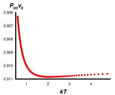
Figure 1: Non-monotonic behavior of $v_{0}P_{\text{int}}$ with $kT$ (arbitrary energy scale).

In Fig. 2, we show $P_{\text{IN}}$ (MPa) as a function of the temperature $t_{\text{C}}$ (^∘C) for a pure component ($M=100,$ $q=10,$ $v_{0}=1.6\times 10^{-28}$ m${}^{\text{3}},$ and $e=-2.6\times 10^{-21}~{}$J) for a constant $V$ ($\phi_{0}=0.012246$), and constant $P$ ($1.0$ atm). At 0^∘C, the system has $\phi_{0}=0.012246,$ and $P=1.0$ atm in both cases so that isobaric and isochoric $P_{\text{IN}}$ match there, as seen in Fig. 2. We notice that isochoric $P_{\text{IN}}$ has a very week dependence on $t_{\text{C}}$ (suggesting that the temperature range in Fig. 2 may be near the maximum of $P_{\text{IN}}),$ while isobaric calculation provides a strongly dependent $P_{\text{IN}},$ which asymptotically goes to zero. This difference in the isobaric-isochoric behavior is consistent with our claim above. The difference between the two internal pressures finally reaches a constant equal to about $80$ MPa at very high temperatures. We also show the derivative $(\partial\mathcal{E}/\partial V)_{T}$ calculated for the isochoric case for comparison. We use isochoric $P_{\text{IN}}$ and (25) to obtain isochoric $(\partial\mathcal{E}/\partial V)_{T}.$ We notice that it differs from isochoric $P_{\text{IN}}$ by a small amount over the entire temperature range considered. Near 0^∘C, they differ by about 1 MPa, and this difference decreases as the temperature rises so that they approach each other at higher temperatures. This is consistent with what we learned from Fig. 1 above. We also notice that $P_{\text{IN}}>(\partial\mathcal{E}/\partial V)_{T}$ over the temperature range in Fig. 2, and the difference gradually vanishes. From (25), we conclude that $(\partial P_{\text{IN}}/\partial T)>0$ for this to be true. This corresponds to $(\partial P_{\text{int}}/\partial T)<0$ in Fig. 2. Thus, the temperature range is below the minimum of$\ P_{\text{int}}$; refer to Fig. 1.

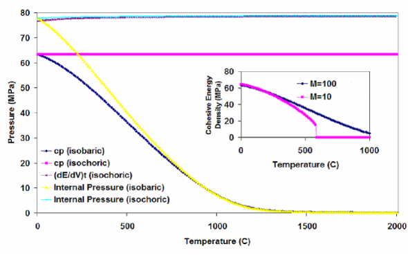
Figure 2: Various isochoric and isobaric pressures vs temperature for a pure component $(M=100,q=10,v_{0}=1.6\times 10^{-28}m^{\text{3}},$and $e=-2.6\times 10^{-21}~{}J)$. In the inset, we show cohesive pressure at $1.0$ atm for two different $M$ ($M=100:$component 1 and $M=10:$component 2), with the smaller $M$ showing a discontinuity at its boiling point around $600^{\circ}$C.

IV Pure Component Cohesive Energy Density or Pressure

IV.1 Athermal Reference State

The following discussion in this section is general and not restricted to a lattice except for the numerical results, which are on a lattice. Therefore, we will include the kinetic energy of the system in this discussion. The definition of $\delta$ requires considering a pure component consisting of one particular component. To be specific, we consider this to be the component $i=1,$ and we will not exhibit the index unless needed for clarity. At a given temperature $T$, and pressure $P$ or volume $V$, one calculates the interaction energy $E_{\text{int}}$ per unit volume by subtracting the kinetic energy $K$ due to motion from the total internal energy $\mathcal{E}$ of the system. We will assume in the following that the interaction energy depends only on the coordinates and not on the momenta of the particles. In classical statistical mechanics, $K$ is a function only of the temperature $T$ but not of the volume Fedor , and can be obtained by considering a fictitious pure component at the same $T$, and $P$ (or $V$), containing the same number of particles, but with particles having no interaction ($U=0$). This fictitious reference system is, as said above, known as the athermal reference state. Then, $K=\mathcal{E}_{\text{ath}},$ where $\mathcal{E}_{\text{ath}}$ is the energy of the athermal system. This reference state is equivalent to the conventional view according to which one considers the gaseous state of the system at the same $T$, but at zero pressure, so that $V\rightarrow\infty,$ which allows for infinite separation between particles to ensure $\mathcal{E}_{\text{int}}=0.$ The energy of the gaseous state is exactly $\mathcal{E}_{\text{ath}},$ which is independent of the volume, even though the physical state requires $V\rightarrow\infty$ for the absence of interactions. We will continue to use the athermal system instead of the gas phase since the latter requires considering different pressure or volume than the pressure or volume of the physical system under consideration. Thus, we find from (1)

$$E_{\text{int}}\equiv E-(V_{\text{ath}}/V)E_{\text{ath}},$$

where $E\equiv\mathcal{E}/V$ is the energy density of the pure component (with interactions), and $E_{\text{ath}}\equiv\mathcal{E}_{\text{ath}}/V_{\text{ath}}$ is the energy density of the athermal reference state ($e\equiv e_{11}=0$), and $V$ and $V_{\text{ath}}$ are the corresponding volumes. As said above, $E_{\text{int}}$ has different limits at infinite temperatures depending on whether we consider an isochoric or isobaric process.

IV.2 Cohesive Energy Density

The cohesive density $c^{\text{P}}$ is the interaction energy of the particles in the pure component. We set $e\equiv e_{11},$ which must be negative for cohesion. The cohesive energy density $c^{\text{P}}$ for the pure component can be thought of as functions of $T$, and $P,$ or $T$, and $V,$ as the case may be. It is obvious that $E_{\text{int}}$ vanishes as the interaction energy $e$ vanishes. This will also be a requirement for the cohesive energy density: $c^{\text{P}}$ should vanish with the interaction energy. We have calculated $c^{\text{P}}$ as a function of $T$ for isochoric (constant volume) and for isobaric (constant pressure) processes. We denote the two quantities by $c_{V}^{\text{P}}$ and $c_{P}^{\text{P}},$ respectively, and show them in Fig. 2, where they can also be compared with $P_{\text{IN}}$ for isochoric and isobaric processes, respectively. The conditions for the two processes are such that they correspond to identical states at $0^{\circ}$C. We find that while the two quantities $c^{\text{P}}$ and $P_{\text{IN}}$ are very different for the two processes, they are similar for each process. We again note that $c_{V}^{\text{P}}$ and $c_{P}^{\text{P}}$ behave very differently, as discussed above, with $c_{V}^{\text{P}}$ $\geq$ $c_{P}^{\text{P}}.$ Not surprisingly, the same inequality also holds for $P_{\text{IN}}.$

The almost constancy of isochoric $c^{\text{P}}$ and $P_{\text{IN}}$ provides a strong argument in support of their usefulness as a suitable candidate for the cohesive pressure. This should not be taken to imply that $c^{\text{P}}$ and $P_{\text{IN}}$ remain almost constant in every process, as the isobaric results above clearly establish. Unfortunately, most of the experiments are done under isobaric conditions; hence the use of isochoric cohesive quantities may not be useful, and even misleading and care has to be exercised.

In the lattice model with only nearest-neighbor interactions, $E_{\text{int}}=e\phi_{\text{c}}$ where $\phi_{\text{c}}\equiv\phi_{11}$ is the contact density between monomers (of component $i=1);$ hence

$$\delta^{2}\equiv c^{\text{P}}\equiv-e\phi_{\text{c}}/v_{0}.$$ (27)

RMA Limit

In the RMA limit, we find from (23) that

$$c^{\text{P}}\ {}^{\underrightarrow{\text{RMA}}}\ -qe\phi_{\text{m}}^{2}/2v_{0},$$ (28)

where $\phi_{\text{m}}$ represents the pure component monomer density in this section. We thus find that the ratio

$$c^{\text{P}}/qe\phi_{\text{m}}^{2}\overset{\text{RMA}}{=}\text{const}$$

in this limit. Since in this limit, the product $qe$ remains a constant, the ratio

$$\widetilde{c}\equiv c^{\text{P}}/\phi_{\text{m}}^{2}\overset{\text{RMA}}{=}\text{const}$$

in this limit. Both these properties will not hold true in general.

End Group Effects

In the following, we will study the combinations

$$\widehat{c}\equiv 2c^{\text{P}}v_{0}/(q-2\nu)e\phi_{\text{m}}^{2},c^{\prime}\equiv c^{\text{P}}/(q-2\nu)$$ (29)

which incorporate the end group effects along with the linear connectivity via the correction $2\nu,$ where

$$\nu\equiv(M-1)/M.$$

In the RMA limit,

$$\widehat{c}\ ^{\underrightarrow{\text{RMA}}}\ 1,$$

and

$$c^{\prime}/e\ ^{\underrightarrow{\text{RMA}}}\ \phi_{\text{m}}^{2}/2v_{0}.$$

We will investigate how close $\widehat{c}$ is to $1$ in our calculation for finite $q,$ and how close to a quadratic form in terms of $\phi_{\text{m}}$ does $c^{\prime}$ have.

IV.3 van der Waals Fluid

To focus our attention, let us consider a fluid which is described by the van der Waals equation. It is known that for this fluid, $E_{\text{int}}=-N_{\text{P}}^{2}a/V^{2},$ where $a>0$ is determined by the integral Landau

$$a\equiv-(1/2)\int_{2r_{0}}^{\infty}udV;$$ (30)

here $u$ is a two-body potential function. It is clear that $a$ is independent of $T$ for the van der Waals fluid. We can also treat it to be independent of $V\ ($any $V$-dependence must be very weak and can be neglected). The lower limit of the integral is the zero of the two-body potential energy. Thus,

$$c^{\text{P}}=an_{\text{P}}^{2},$$ (31)

where $n_{\text{P}}$ is the number density per unit volume; for polymers, $n_{\text{P}}\equiv\phi_{\text{m}}/Mv_{0}$. It is interesting to compare (31) with (28) derived in the RMA limit. They both show the same quadratic dependence on the number density. We also note that $c^{\text{P}}$ vanishes as $a$ vanishes, as we expect, but most importantly the ratio $c^{\text{P}}/n_{\text{P}}^{2}$ is independent of the temperature, just as $\widetilde{c}$ is a constant in the RMA limit. Deviation from the quadratic dependence will be observed in most realistic systems, since they cannot be described by this approximation.

An interesting observation about this fluid is that $P_{\text{int}}$ is exactly equal to $E_{\text{int}};$ thus, $c^{\text{P}}=-P_{\text{int}}$ for this fluid. In addition, it is well known that for this fluid

$$(\partial\mathcal{E}/\partial V)_{T}=(\partial\mathcal{E}_{\text{int}}/\partial V)_{T}=an_{\text{P}}^{2},$$ (32)

since $a$ is temperature-independent. Thus,

$$P_{\text{IN}}\equiv(\partial\mathcal{E}/\partial V)_{T}$$ (33)

for the the van der Waals fluid, in which $a$ must be taken as $T$-independent. The equality (33) is not always valid as discussed above.

IV.4 The Usual Approximation

Usually, one approximates $E_{\text{int}}$ by the energy density of vaporization at the boiling point at $T=T_{\text{B}}.$ This means that one approximates $c^{\text{P}}(T,P)$ by its value $c^{\text{P}}(T_{\text{B}},P),$ which will be a function of $P$, but not of $T.$ On the contrary, $c^{\text{P}}(T,P)$ will show variation with respect to both variables. In addition, it will also change with the lattice coordination number $q,$ and the interaction energy $e$. It is clear that isobaric $c^{\text{P}}(T,P)$ will show the discontinuity at the boiling point, as shown in the inset in Fig. 2, where we report isobaric $c^{\text{P}}$ for two different molecular weights $M=10,$ and $M=100$ at $1.0$ atm. The shorter polymer system boils at about $600^{\circ}$C (and $1.0$ atm$)$, but not the longer polymer over the temperature range shown there. At $0^{\circ}$C, the smaller polymer has a slightly higher value of isobaric $c^{\text{P}}.$ If we calculate isochoric $c^{\text{P}}$ at a volume equal to that in the isobaric case at $0^{\circ}$C and $1.0$ atm, then the corresponding isochoric $c^{\text{P}},$ which is almost a constant (as shown in the main figure in Fig. 2), will be about $65$ MPa, close to its value at $0^{\circ}$C. This value is much larger than $c^{\text{P}}(T_{\text{B}},P)$ of about $15$ MPa at the boiling point. Thus, the conventional approximation cannot be taken as a very good estimate of the cohesiveness of the system, which clearly depends on the state of the system.Cohesive energy density as a function of pressure for different $q$.

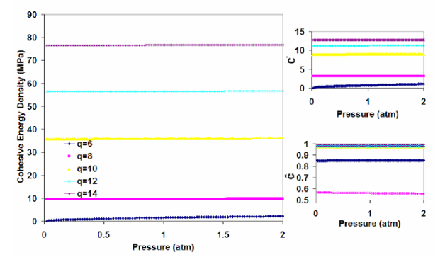
Figure 3: Cohesive energy density as a function of pressure for different $q$. We also show $c^{\prime}$ and $\widehat{c}.$

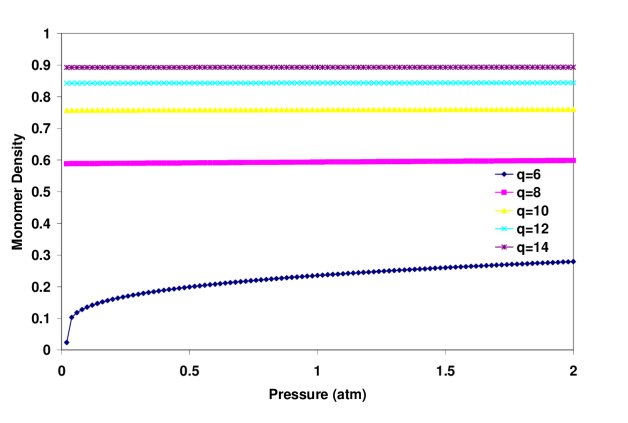
Figure 4: Monomer density as a function of presssure for different $q$. For $q\geq 8,$ we have a liquid which gets denser as $q$ increases. For $q=6,$ we have a gas phase at low pressure which becomes a lighter liquid at higher pressure, with a liquid gas transition around 0.05 atm.

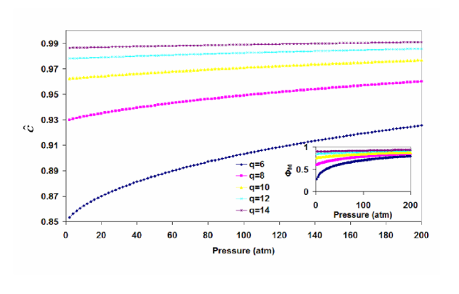
Figure 5: $\widehat{c}$ as a function of pressure at $500^{\circ}$C for different $q$. As $q$ increases, $\widehat{c}$ approaches $1,$ its limiting RMA value, which also forms its upper limit. For any finite $q$, $\widehat{c}$ is strictly lower.

IV.5 Numerical results

We will evaluate various quantities for isochoric and isobaric processes. For isochoric calculations, we calculate $\phi_{\text{m}}$ at some reference $T,P.$ Usually, we take it to be at $1^{\circ}$C, and $1.0$ atm. We then keep $\phi_{\text{m}}$ fixed as we change the temperature. This is equivalent to keeping the volume fixed for a given amount of the polymers. For isobaric (constant $P$) calculations, we again start at $1^{\circ}$C, and take a certain pressure such as $1.0$ atm, and keep the pressure fixed by adjusting $\phi_{\text{m}}$ as we change the temperature. For a given amount of polymers, this amounts to adjusting the volume of the system.

We show $c^{\text{P}}$ in Fig. 3, and the monomer density $\phi_{\text{m}}$ in Fig. 4, as a function of $P$ ($P\leq 2$ atm) for different values of $q$ from $q=6$ to $q=14.$ We have taken $M=500,$ $v_{0}=1.6\times 10^{-28}$ m${}^{\text{3}},$ and $e=-2.6\times 10^{-21}~{}$J, and have set $t_{\text{C}}=500^{\circ}$C. We see that $c^{\text{P}}$ increases with $q$, which is expected; see (28). To further analyze this dependence, we plot $c^{\prime}$ in Fig. 3. There is still a residual increase with $q.$ The increase is also partially due to the fact that $\phi_{\text{m}}$ increases with $q,$ as shown in Fig. 4. Therefore, we also plot $\widehat{c}$ as a function of $P$ in Fig. 3. We notice that there is still a residual dependence on $q$ with $\widehat{c}$ increasing with $q,$ and reaching $1.0$ from below as $q$ increases, which is consistent the RMA limit. In Fig. 5, we plot $\widehat{c}$ and $\phi_{\text{m}}$ (in the inset) for the same system over a much wider range of pressure for different $q.$ From the behavior of $\ \widehat{c}$ and $\phi_{\text{m}},$ we easily conclude that $c^{\text{P}}$ changes strongly with $P$ for smaller $q,$ and the dependence gets weaker as $q$ increases.

In Fig. 6, we plot $c^{\text{P}}$ for $q=12$ as a function of the monomer density $\phi_{\text{m}}.$ We have taken $M=500,$ $v_{0}=1.6\times 10^{-28}$ m${}^{\text{3}},$ and $e=-2.6\times 10^{-21}~{}$J, and have set $t_{\text{C}}=500^{\circ}$C. According to (28), it should be a quadratic function of the monomer density. To see if this is true for the present case of finite $q,$ we plot the ratio $c^{\text{P}}/\phi_{\text{m}}^{2}$ in the inset, which clearly shows that there is still a strong residual dependence left in the ratio. Thus, $c^{\text{P}}$ in a realistic system should not be quadratic in $\phi_{\text{m}}.$

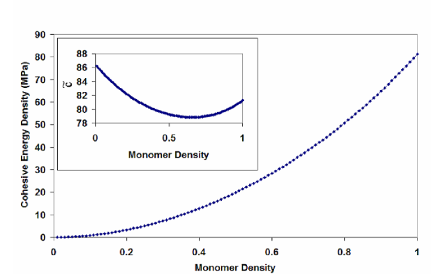
Figure 6: $c^{\text{P}}$ as a function of $\phi_{\text{m}}.$ In the inset, we show $\widetilde{c},$ showing that $c^{\text{P}}$ is not quadratic in $\phi_{\text{m}},$ as suggested by the regular solution theory.

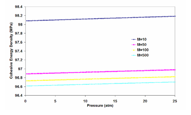
Figure 7: Cohesive energy density as a function of pressure for different molecular weights.

In Fig. 7, we show $c^{\text{P}}$ as a function $P$ for small pressures for different $M$ ranging from $M=10$ to $M=500;$ we keep $q=14,$ $v_{0}=1.6\times 10^{-28}$ m${}^{\text{3}},$ and $e=-2.6\times 10^{-21}~{}$J, and have set the temperature $t_{\text{C}}=25^{\circ}$C. We see that $c^{\text{P}}$ decreases as $M$ increases, but different curves are almost parallel, indicating that it is not the slope, but the magnitude that is affected by $M.$ In Fig. 8, we show $c^{\text{P}}$ as a function $P$ for small pressures for different temperatures ranging from $t_{\text{C}}=25^{\circ}$C to $t_{\text{C}}=5000^{\circ}$C; we keep $q=14,$ $M=100,~{}v_{0}=1.6\times 10^{-28}$ m${}^{\text{3}},$ and $e=-2.6\times 10^{-21}~{}$J. We immediately note that the pressure variation is quite minimal over such a small range of pressure between 1 to 25 atm. However, the temperature variation is quite pronounced, again affecting the magnitude and not the slope. There are two important observations. (i) For the highest temperature $5000^{\circ}$C, the state corresponds to a gas, since $c^{\text{P}}\simeq 0.$ (ii) At low temperatures, $c^{\text{P}}$ reaches an asymptotic value since the system has become almost incompressible.

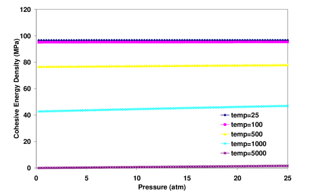
Figure 8: Cohesive energy density as a function of pressure at different temperatures.

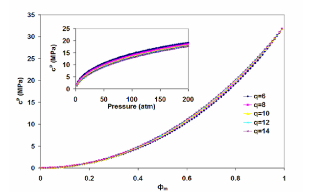
Figure 9: $c^{\text{P}}$ as a function of $\phi_{\text{m}}$ for different $q$ when $e(q/2-\nu)$ is kept fixed at ($-5.21\times 10^{-21}$J).

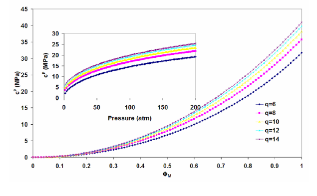
Figure 10: $c^{\text{P}}$ as a function of $\phi_{\text{m}}$ for different $q$ when $eq$ is kept fixed at ($-1.56\times 10^{-20}$J).

In Fig. 9, which is for a pure component studied in Fig. 3, we keep the product $e(q/2-\nu)$ fixed at ($-5.21\times 10^{-21}$J), as we change $q$, so that $e$ changes with $q.$ We keep $M=500,$ $v_{0}=1.6\times 10^{-28}$ m${}^{\text{3}},$ and $t_{\text{C}}=500^{\circ}$C. The effect of changing $q$ is now minimal. The cohesive energy density shows minimal variation with $q$, except that it is higher for larger $q$, but the difference first increases with $\phi_{\text{m}}$ and then decreases as $\phi_{\text{m}}\rightarrow 1.$ In Fig. 10, we keep instead the product $eq$ fixed, so that there is no endpoint correction. In contrast with Fig. 9, we find that $c^{\text{P}},$ while still increasing with $q$, has the property that the its difference for different $q$ continues to increases with $\phi_{\text{m}}$ as $\phi_{\text{m}}\rightarrow 1.$ It is clear from both figures that $c^{\text{P}}$ increases with $q$ at a given $\phi_{\text{m}}$ and saturates as $q$ becomes large, which is the direction in which $q$ must increase to obtain the RMA limit. Thus, $c^{\text{P}}$ achieves its maximum value at a given density $\phi_{\text{m}}$ in the RMA approximation: for any realistic system in which $q$ is some finite value, the value of the cohesive energy at that density $\phi_{\text{m}}$ will be strictly smaller. It is also evident from the inset in both figures that at a given pressure $P$, $c^{\text{P}}$ achieves its minimum value in the RMA approximation.

The results for isochoric and isobaric calculations are shown in Fig. 11. We consider $q=14,$ $M=100,~{}v_{0}=1.6\times 10^{-28}$ m${}^{\text{3}},$ and $e=-2.6\times 10^{-21}~{}$J, and have taken the pressure to be $P=1.0$ atm at the initial temperature $t_{\text{C}}=0^{\circ}$C. This corresponds to the monomer density $\phi_{\text{m}}=0.997115.$ For the isochoric calculation, we maintain the same monomer density ($\phi_{\text{m}}=0.997115$) at all temperatures. For the isobaric calculation, we maintain the same pressure ($P=1$ atm) at all temperatures. This ensures that isochoric $c_{V}^{\text{P}}$  and isobaric $c_{P}^{\text{P}}$ are identical at $t_{\text{C}}=0^{\circ}$C. The figure clearly shows that $c_{V}^{\text{P}}$ is always higher than $c_{P}^{\text{P}}$, as discussed above. This behavior is not hard to understand. As we raise $T$, the pressure increases in the constant volume calculation above $P=1$ atm, making particles get closer together, thereby increasing the cohesive energy.

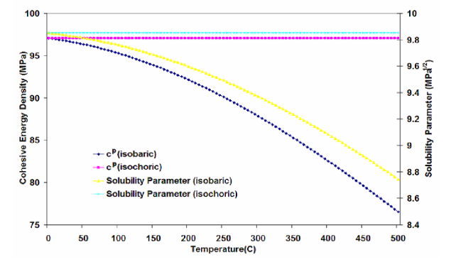
Figure 11: Various $c^{\text{P}}$ as a function of temperature.

V Mutual Cohesive Energy Density or Pressure

V.1 Mutual Interaction

The solubility of one of the components in a binary mixture of components $i=1,2$ increases as the excess energy $\varepsilon_{12}$ decreases for the simple reason that a larger $\varepsilon_{12}$ corresponds to a stronger excess repulsion between the two components. In particular, the two components will not phase separate at any temperature if $\varepsilon_{12}\leq 0$. If $\varepsilon_{12}>0,$ the two components will phase separate at low temperatures. Thus, knowing whether $\varepsilon_{12}>0$ immediately allows us to conclude that solubility will not occur everywhere.

Usually, all energies $e_{ij}$ are negative, but the sign of $\varepsilon_{12}$ depends on their relative magnitudes. If, however, we assume the London conjecture (11), then the corresponding excess energy becomes

$$\varepsilon_{12}=(\sqrt{\left|e_{11}\right|}-\sqrt{\left|e_{22}\right|})^{2}/2\geq 0.$$ (34)

Thus, the London conjecture implies that the two components experience a repulsive excess interaction so that the solubility decreases as $\varepsilon_{12}$ increases, i.e., as $e_{11}$ and $e_{22}$ become more disparate. The maximum solubility in this case occurs when $\varepsilon_{12}=0,$ i.e., when the two components have identical interactions (”like dissolves like”). In this case, the size or architectural disparity cannot diminish the solubility because the entropy of mixing will always promote miscibility. In general, $\varepsilon_{12}>0,$ and it becomes necessary to study solubility under different thermodynamic conditions.

To simplify our investigation, we will assume the London conjecture (11) for the mixture in all the calculations. Thus, the two components always experience a repulsive excess interaction in our calculation. (This is also true when we intentionally violate the London conjecture (11) and set $e_{12}=0,$ as is the case for SRS.) In the RMA limit, the conjecture (11) immediately leads to (10), as we have seen above. This need not remain true when we go beyond RMA. Thus, we will inquire if (10) is satisfied in general for cohesive energies that are calculated from our theory under the assumption that the London conjecture (11) is valid. Any failure of (10) under this condition will clearly have significant implications for our basic understanding of solubility.

V.2 van Laar-Hildebrand Approach using Energy of Mixing

We follow van Laar vanLaar and Hildebrand Hildebrand , and introduce $c_{12}$ by exploiting the energy of mixing $\Delta E_{\text{M}}$ per unit volume. According to the isometric regular solution theory Hildebrand , the two are related by

$$\Delta E_{\text{M}}=(c_{11}^{\text{P}}+c_{22}^{\text{P}}-2c_{12})\varphi_{1}\varphi_{2},$$ (35)

where $\varphi_{i}$ are supposed to denote the volume fractions. Using the London-Berthelot conjecture (10), we immediately retrieve (3), once we recognize that $\delta_{1}^{2}\equiv c_{11}^{\text{P}},$ and $\delta_{2}^{2}\equiv c_{22}^{\text{P}},$ see (2) above. We now take (35) as the general definition of the mutual cohesive energy density $c_{12}$ in terms of the pure component cohesive energy densities. The extension then allows us to evaluate $c_{12}$ by calculating $\Delta E_{\text{M}},$ provided we know $c_{11}^{\text{P}}$ and $c_{22}^{\text{P}}$ for the pure components; the latter are independent of the composition. It can be argued that since (35) is valid only for isometric mixing, it should not be considered a general definition of $c_{12}$ for non-isometric mixing. However, since one of our objectives is to investigate the effects due to isometric and non-isometric mixing, we will adopt (35) as the general definition of $c_{12}.$

V.2.1 Lattice model

The kinetic energy of the mixture is the sum of the kinetic energies of the pure components, all having the same temperature, and will not affect the energy of mixing. Thus, we need not consider the kinetic energy in our consideration anymore. In other words, we can safely use a lattice model in calculating $\Delta E_{\text{M}}.$ This is what we intend to do below.

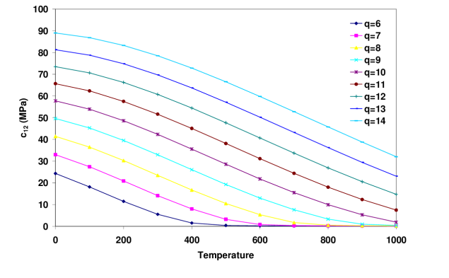
Figure 12: Mutual cohesive energy density as a function of temperature for different $q.$ We have taken a blend at 50-50 composition ($M_{1}=M_{2}=100;e_{11}=-2.2\times 10^{-21}$ J, $e_{22}=-2.6\times 10^{-21}$ J, $v_{0}=1.6\times 10^{-28}$ m³) at 1.0 atm.

The definition of $c_{12}$ depends on a form (35) whose validity in general is questionable, as it is based on RST. To appreciate this more clearly, let us find out the conditions under which the RMA limit of our recursive theory will reproduce (35). We first note that the interaction energy density (per unit volume) $E_{\text{int}}$ of the mixture from (20) is given by

$$E_{\text{int}}v_{0}\equiv e_{11}\phi_{11}+e_{22}\phi_{22}+e_{12}\phi_{12}=-c_{11}^{\text{P}}v_{0}\phi_{11}/\phi_{11}^{\text{P}}-c_{22}^{\text{P}}v_{0}\phi_{22}/\phi_{22}^{\text{P}}+e_{12}\phi_{12},$$ (36)

where we introduced the pure component cohesive energy densities in the last equation. The energy of mixing per unit volume is

$$\Delta E_{\text{M}}v_{0}=e_{11}\phi_{11}+e_{22}\phi_{22}+e_{12}\phi_{12}-(V_{1}^{\text{P}}/V)e_{11}\phi_{11}^{\text{P}}-(V_{2}^{\text{P}}/V)e_{22}\phi_{22}^{\text{P}},$$ (37)

where $V_{1}^{\text{P}},$ and $V_{2}^{\text{P}}$ are the pure component volumes. It is easy to see that in general

$$V_{1}^{\text{P}}/V=x\phi_{\text{m}}/\phi_{\text{m}1}^{\text{P}}\equiv\phi_{\text{m1}}/\phi_{\text{m}1}^{\text{P}},V_{2}^{\text{P}}/V=(1-x)\phi_{\text{m}}/\phi_{\text{m}2}^{\text{P}}\equiv\phi_{\text{m2}}/\phi_{\text{m}2}^{\text{P}},$$ (38)

where $x\equiv\phi_{\text{m1}}/\phi_{\text{m}}$ is the monomer fraction of species $i=1$ introduced earlier in (4),and $\phi_{\text{m}i}^{\text{P}}$ the pure component monomer density of the $i$th species. The monomer density of both species in the mixture is $\phi_{\text{m}}\equiv\phi_{\text{m1}}+\phi_{\text{m2}}$.

V.2.2 RMA Limit and Monomer Density Equality:

In the RMA limit, it is easy to see by the use of (22b) that the last equation in (36) reduces to

$$E_{\text{int}}~\ {}^{\underrightarrow{\text{RMA}}}~{}-c_{11}^{\text{P}}(V_{1}^{\text{P}}/V)^{2}-c_{22}^{\text{P}}(V_{2}^{\text{P}}/V)^{2}-2c_{12}(V_{1}^{\text{P}}/V)(V_{2}^{\text{P}}/V),$$

where

$$c_{ii}^{\text{P}}~\ {}^{\underrightarrow{\text{RMA}}}-(1/2)qe_{ii}\phi_{\text{m}i}^{\text{P}2}/v_{0},\text{ }c_{12}\ \ ^{\underrightarrow{\text{RMA}}}\ -qe_{12}\phi_{\text{m}1}^{\text{P}}\phi_{\text{m}2}^{\text{P}}/2v_{0}$$ (39)

are the cohesive energy densities in this limit. The form of $c_{ii}^{\text{P}}$ is exactly the same as the one derived above for the pure component; see (23), and (31). It is also a trivial exercise to see that the RMA limit of the energy of mixing (37) will exactly reproduce (35) provided we identify

$$\varphi_{1}\equiv V_{1}^{\text{P}}/V,\varphi_{2}\equiv V_{2}^{\text{P}}/V\text{ ,}$$

and further assume

$$\text{ }V_{2}^{\text{P}}+V_{2}^{\text{P}}=V,$$

so that $\varphi_{1}+$ $\varphi_{2}=1.$ The last condition is nothing but the requirement that mixing be isometric and can be rewritten using (38) as

$$\phi_{\text{m}}\phi_{\text{m}1}^{\text{P}}+x\phi_{\text{m}}(\phi_{\text{m}2}^{\text{P}}-\phi_{\text{m}1}^{\text{P}})\equiv\phi_{\text{m}1}^{\text{P}}\phi_{\text{m}2}^{\text{P}}.$$

This should be valid for all $x$ including $x=0$ and $x=1.$ This can only be true if we require the monomer density equality:

$$\phi_{\text{m}}=\phi_{\text{m}1}^{\text{P}}=\phi_{\text{m}2}^{\text{P}}.$$ (40)

This condition is nothing but the equality of the free volume densities in the mixture and the pure components, and is a consequence of isometric mixing, as is easily seen from (45a) obtained below. We finally conclude that

$$\varphi_{1}\equiv x,\varphi_{2}\equiv 1-x,$$ (41)

as was also the case discussed earlier in the context of (3).

V.2.3 Isometric RMA Limit

Let us now consider the isometric RMA limit for which we have the simplification

$$V_{1}^{\text{P}}/V=x,V_{2}^{\text{P}}/V=1-x;$$

see (40). Thus,

$$E_{\text{int}}\ {}^{\underrightarrow{\text{RMA}}}\ -[c_{11}^{\text{P}}\varphi_{1}^{2}+2c_{12}\varphi_{1}\varphi_{2}+c_{22}^{\text{P}}\varphi_{2}^{2}],$$

as is well known Hildebrand . This form can only be justified in the isometric RMA limit, with the volume fractions given by (41). Similarly,

$$\Delta E_{\text{M}}v_{0}\ {}^{\underrightarrow{\text{RMA}}}\ q[e_{12}-(1/2)(e_{11}+e_{22})]\phi_{\text{m}1}\phi_{\text{m}2}=(\chi/\beta)\phi_{\text{m}1}\phi_{\text{m}2},$$

where we have introduced the Flory-Huggins chi parameter $\chi\equiv q\beta\varepsilon.$ Using (40), we can rewrite the above energy of mixing in the form (35). We finally have for $\Delta E_{\text{M}}$ in the isometric RMA limit

$$\Delta E_{\text{M}}\ {}^{\underrightarrow{\text{RMA}}}\ (\chi\phi_{\text{m}}^{2}/\beta v_{0})\varphi_{1}\varphi_{2},$$ (42)

again with the volume fractions given by (41).

V.2.4 Volume Fractions

In the following, we will always take $\varphi_{i}$ to be given by (41). This ensures that $\varphi_{1}+$ $\varphi_{2}=1.$ Another possibility is to define $\varphi_{i}$ in terms of partial monomer volumes $\overline{v_{i}}$:

$$\varphi_{i}\equiv\phi_{\text{m}i}\overline{v_{i}}/v_{0}.$$ (43)

However, as shown in RaneGuj2003 , the error is not significant except near $x=0$ or $x=1$. Since the calculation of $\overline{v_{i}}$ is somewhat tedious, we will continue to use (41) for $\varphi_{i}$ in our calculation, as we are mostly interested in $x=0.5$.

V.2.5 Beyond Isometric RMA

Beyond isometric RMA, the energy of mixing will not have the above form in (42); rather, it will be related to the energetic effective chi introduced in (9) Gujrati1998 ; Gujrati2003 in exactly the same form as above:

$$\Delta E_{\text{M}}\equiv(\chi_{\text{eff}}^{\text{E}}\phi_{\text{m}}^{2}/\beta v_{0})\varphi_{1}\varphi_{2},$$

which ties the concept of cohesive energy density intimately with that of the effective chi, as noted earlier. However, it is also clear that $c_{12}$ and $\chi_{\text{eff}}^{\text{E}}$ are not directly proportional to each other.

V.3 van Laar-Hildebrand $c_{12}$

Using (27) for pure component cohesive energies, we obtain

$$c_{12}v_{0}=(e_{12}/2)\phi_{12}-e_{11}[(\phi_{11}-V_{1}^{\text{P}}/V\phi_{11}^{\text{P}})/2\varphi_{1}\varphi_{2}-\phi_{11}^{\text{P}}]-e_{22}[(\phi_{22}-V_{2}^{\text{P}}/V\phi_{22}^{\text{P}})/2\varphi_{1}\varphi_{2}-\phi_{22}^{\text{P}}]$$ (44)

as the general expression for the cohesive energy density. We will assume that $\varphi_{i}$ are as given in (41). It is clear that the definition of $c_{12}$ given in (35) is such that it not only depends on the state of the mixture, but also depends on pure component states. This is an unwanted feature. In particular, $c_{12}$ will show a discontinuity if a pure component undergoes a phase change (see Fig. 23 later), even though the mixture does not.

In Fig. 12, we show $c_{12}$ for a 50-50 blend ($M=100$) at $1.0$ atm as a function of $t_{\text{C}}$ calculated for different values of $q$ from $q=6$ to $q=14.$ The curvature of $c_{12}$ gradually changes at low temperatures from concave upwards to downwards. As not only the magnitude but also the shape of $c_{12}$ changes with $q$, $c_{12}$ is not simply proportional to $q$; it is a complicated function of it. This is easily seen from the values of $c_{12}/q$ at $t_{\text{C}}=0{{}^{\circ}}$C, which is found to increase with $q.$ It is about $4.0$ at $q$=6 and increases to about $6.4$ at $q=14.$ The temperature where $c_{12}$ asymptotically becomes very small, such as $0.1$ MPa occurs at higher and higher values of the temperature as $q$ increases. This is not surprising. We expect the cohesion to increase with $q$ at a given temperature.

V.4 Isometric Mixing: EDIM and DDIM

The volume of mixing is defined as

$$\Delta V_{\text{M}}\equiv V-V_{1}^{\text{P}}-V_{2}^{\text{P}}.$$

Using (38), we find that the volume of mixing per unit volume ($\Delta v_{\text{M}}\equiv\Delta V_{\text{M}}/V$), and per monomer ($\Delta\widehat{v}_{\text{M}}\equiv\Delta V_{\text{M}}/N_{\text{m}}$) are

$$\Delta v_{\text{M}} \equiv\phi_{\text{m}}[1/\phi_{\text{m}}-x/\phi_{\text{m}1}^{\text{P}}-(1-x)/\phi_{\text{m}2}^{\text{P}}],$$ (45a)

$$\Delta\widehat{v}_{\text{M}} \equiv(1/\phi_{\text{m}}-x/\phi_{\text{m}1}^{\text{P}}-(1-x)/\phi_{\text{m}2}^{\text{P}})v_{0}.$$ (45b)

One of the conditions for RST to be valid is that this quantity be zero (isometric mixing). The condition (40), which ensures isometric mixing at all $x$, is much stronger than the isometric mixing requirement at a given fixed value of $x$. There are situations in which mixing is isometric at a given $x$, but (40) is not satisfied. For a given pure component monomer densities $\phi_{\text{m}1}^{\text{P}},$ and $\phi_{\text{m}2}^{\text{P}},$ that are to be mixed at a given composition $x,$ we must choose the mixture density $\phi_{\text{m}}$ to satisfy

$$1/\phi_{\text{m}}=x/\phi_{\text{m}1}^{\text{P}}+(1-x)/\phi_{\text{m}2}^{\text{P}}$$ (46)

in order to make the mixing isometric; see (45a). In this case, (35) will not hold true despite mixing being isometric. In our calculations, we will consider both ways of ensuring isometric mixing. We will call the mixing method satisfying (40) equal density isometric mixing (EDIM), and the mixing method satisfying (46) different density isometric mixing (DDIM).

For most of our computation, we fix the composition $x.$ Almost all of our results are for a 50-50 mixture. We will consider both isometric mixing processes noted above in our calculations. A variety of processes can be considered for each mixing. In order to make calculations feasible, we need to restrict the processes to a few selected ones. We have decided to investigate the following processes with the hope that they are sufficient to illuminate the complex behavior of cohesive energy densities and their usefulness.

V.4.1 (Isometric) Isochoric Process

The process should be properly called an isometric isochoric process, but we will use the term isochoric process in short in this work. The volume of the mixture is kept fixed as the temperature is varied. The energy of mixing can be calculated for a variety of mixing processes. We have decided to restrict this to isometric mixing. We calculate the mixture’s monomer density $\phi_{\text{m}}$ at each temperature. For each temperature, we use (40) to determine the pure component monomer densities to ensure isometric mixing for the selected $x$.

V.4.2 (Isobaric) EDIM Process

The process should be properly called an isobaric EDIM process, but we will use the term EDIM process in short in this work. We keep the mixture at a fixed pressure, which is usually $1.0$ atm, and calculate its monomer density $\phi_{\text{m}}$ at each temperature. We then use EDIM to ensure isometric mixing at each temperature and calculate the energy of mixing. In the process, the mixture’s volume keeps changing, and the pure component pressures need not be at the mixture’s fixed pressure. Thus, the mixing is not at constant pressure, even though the mixture’s pressure is constant.

V.4.3 DDIM Process

For DDIM, we keep the pressures of the pure components fixed, which is usually $1.0$ atm, and calculate $\phi_{\text{m}1}^{\text{P}},$ and $\phi_{\text{m}2}^{\text{P}},$ from which we calculate $\phi_{\text{m}}$ using (46) for the selected $xv$. This ensures isometric mixing, but again the mixing process is not a constant pressure one since the mixture need not have the same fixed pressure of the pure components. Even though the energy of mixing is calculated for an isometric mixing, it is neither calculated for an isobaric nor an isochoric process.

All the above three mixing processes correspond to isometric mixing at each temperature. Thus, we can compare the calculated van Laar-Hildebrand $c_{12}$ for these three processes to assess the importance of isometric mixing on $c_{12}$. It is not easy to consider EDIM for an isochoric (constant $V$) process. Therefore, we have not investigated it in this work.

V.4.4 Isobaric Process

In this process, the pressure of the mixture is kept constant as the temperature is varied. The calculation of the energy of mixing can be carried out for a variety of mixing. We will restrict ourselves to mixing at constant pressure so that the pure components also have the same pressure as the mixture at all temperatures. Thus, the volume of mixing will not be zero in this case. The process is properly described as a constant pressure mixing isobaric process, but we will use the term isobaric process in short in this work.

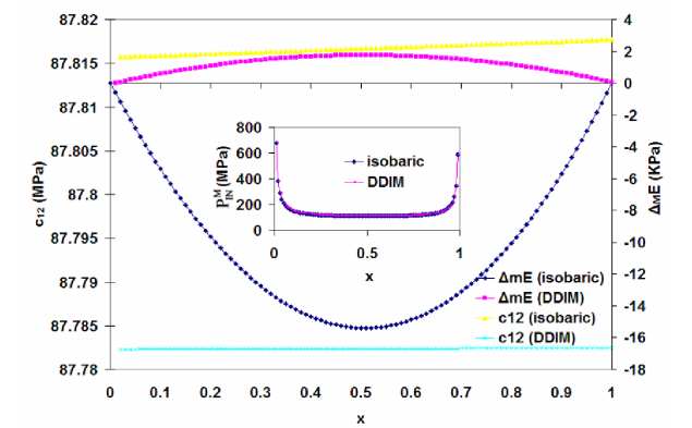
Figure 13: Energy of mixing and mutual cohesive energy density as a function of composition $x$. We take $M_{1}=10,M_{2}=100$, $e_{11}=e_{22}=e_{12}=-2.6\times 10^{-21}$ J, $v_{0}=1.6\times 10^{-28}$ m${}^{\text{3}}$ and $q=14.$ The pressure and temperature are fixed at $1.0$ atm and $300^{\circ}$C, respectively.

V.5 Results

V.5.1 Size Disparity Effects

The effects of size disparity alone are presented in Fig. 13, where we show the energy of mixing as a function of $x=\phi_{\text{m}1}/\phi_{\text{m}}$ for a blend ($M_{1}=10,M_{2}=100$) with $e_{11}=e_{22}=e_{12}=-2.6\times 10^{-21}$ J, so that $\varepsilon_{12}=0.$ Thus, energetically, there is no preference. We take $q=14,$ and the pressure and temperature are fixed at $1.0$ atm and $300^{\circ}$C, respectively. We show isobaric and DDIM results. While the energy of mixing is negative for the isobaric case, which does not correspond to isometric mixing, it is positive everywhere for DDIM, which does correspond to isometric mixing. This result should be contrasted with the Scatchard-Hildebrand conjecture (3) Hildebrand , whose justification requires not only isometric mixing but also the London-Berthelot conjecture (10). We also show corresponding $c_{12}$, which weakly changes with $x.$ For $M_{1}=M_{2}=100,$ the energy and the volume of mixing vanish, which is not a surprising result as we have a symmetric blend (both components identical in size and interaction).

It is important to understand the significance of the difference in the behavior of $\Delta E_{\text{M}}$ for the two processes in Fig. 13. From Fig. 7, we find that the solubility parameter $\delta$ at $1.0$ atm and $25^{\circ}$C is about 9.844 and 9.905 (MPa)^1/2 for $M=100,$ and $10$ respectively. Thus, assuming the validity of the Scatchard-Hildebrand conjecture (3), we estimate $\Delta E_{\text{M}}$ $\cong 0.9$ kPa at equal composition ($x=1/2$). However, a correction for temperature difference needs to made, since the results in Fig. 13 are for $t_{\text{C}}=300^{\circ}$C. From the inset in Fig. 2, we observe that $c^{\text{P}}$ almost decreases by a factor of 2/3, while their difference has increased at $t_{\text{C}}=300^{\circ}$C relative to $t_{\text{C}}=25^{\circ}$C. What one finds is that the corrected $\Delta E_{\text{M}}$ is not far from the DDIM $\Delta E_{\text{M}}$ in Fig. 13 at $x=1/2,$ but has no relationship to the isobaric $\Delta E_{\text{M}},$ which not only is negative but also has a much larger magnitude.

It should be noted that the pressures of the pure components in both calculations reported in Fig. 13 is the same: $1.0$ atm. Under this condition, the Scatchard-Hildebrand conjecture (3) cannot differentiate between different processes as $\delta_{1\text{ }}$and $\delta_{2}$ are unchanged. But this is most certainly not the case in Fig. 13. For a symmetric blend, $\Delta E_{\text{M}}=0$ even in an exact theory. Since the symmetry requires $\delta_{1\text{ }}=\delta_{2},$ we find that the London-Berthelot conjecture (10) is satisfied. Thus, the violation of the Scatchard-Hildebrand conjecture we observe in Fig. 13 is due to non-random mixing caused by size-disparity.

V.5.2 Interaction Disparity Effects

In Fig. 14, we fix $e_{11}=-2.6\times 10^{-21}$ J, and plot the energy of mixing as a function of $(-e_{22})$ for a blend with $M_{1}=M_{2}=100.$ Thus, there is no size disparity but the energy disparity is present except when $e_{11}=e_{22}.$ We not only consider isobaric, and DDIM processes, but also the EDIM process. At $e_{11}=e_{22}$, we have a symmetric blend; hence, $\Delta E_{\text{M}}=0$ and $c_{11}^{\text{P}}=$ $c_{22}^{\text{P}}$ for all the processes. Correspondingly, we have $c_{12}=$ $c_{11}^{\text{P}}$or $c_{22}^{\text{P}},$ and the correction $l_{12}=0$ for all the processes. Away from this point, $\Delta E_{\text{M}}$ for the three processes are different, but remain non-negative. The energy disparity has produced much larger magnitudes of $\Delta E_{\text{M}}$ than the size disparity alone; compare with Fig. 13. This difference in the magnitudes of $\Delta E_{\text{M}}$ is reflected in the magnitudes of $c_{12},$ as shown in the figure. We again find that isobaric and DDIM processes are now quite different; compare the magnitudes of $\Delta E_{\text{M}}$ in Figs. 13 and 14. The difference between DDIM and EDIM, though relatively small, is still present, again proving that isometric mixing alone is not sufficient to validate the Scatchard-Hildebrand conjecture. [We note that $\Delta E_{\text{M}}$ can become negative (results not shown) if we add size disparity in addition to the interaction disparity.] The non-negative $\Delta E_{\text{M}}$ is due to the absence of size disparity, and is in accordance with the Scatchard-Hildebrand conjecture. Since $\Delta E_{\text{M}}$ is the highest for DDIM, the corresponding $c_{12}$ is the lowest. Similarly, the isobaric energy of mixing is usually the lowest, and the corresponding $c_{12}$ usually the highest. We note that all $c_{12}$’s continue to increase with $\left|e_{22}\right|.$ We observe that isobaric and EDIM $c_{12}$’s are closer to each other, and both are higher than DDIM $c_{12}$. In the inset, we also show $l_{12},$ and we learn that it is not a small correction to the London-Berthelot conjecture (10) for the isobaric case (non-isometric mixing). For isometric mixing, we have the usual behavior: a small correction $l_{12}.$

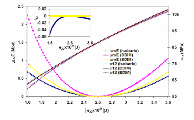
Figure 14: Energy of mixing, mutual cohesive energy density, and correction $l_{12}$ as a function of  $\left|e_{22}\right|$ for a 50-50 blend. We take $M_{1}=M_{2}=100$, $e_{11}=-2.6\times 10^{-21}$ J, $v_{0}=1.6\times 10^{-28}$ m${}^{\text{3}}$ and $q=14.$ The pressure and temperature are fixed at $1.0$ atm and $300^{\circ}$C, respectively.

V.5.3 Variation with $P$

We plot $\Delta E_{\text{M}},$ $c_{12},$ and $l_{12}$ as a function of $P$ in Fig. 15 for isobaric, DDIM, and EDIM processes. We note that all these quantities have a weak but monotonic dependence on $P$ over the range considered. Again, the isobaric $\Delta E_{\text{M}}$ remains the lowest, and consequently isobaric $c_{12}$ remains the highest over the range considered. As noted above, isobaric and EDIM $c_{12}$’s are closer to each other, but different from DDIM $c_{12}$ over the entire range in Fig. 15. The monotonic behavior in $P$ is correlated with a monotonic behavior in $l_{12}.$ We observe that $l_{12}$ provides a small correction at $300^{\circ}$C over the pressure range considered here. The interesting observation is that isobaric $l_{12}$ provides the biggest correction, while DDIM $l_{12}$ the smallest correction. However, the EDIM $l_{12}$ remains intermediate, just as EDIM $c_{12}$ is.

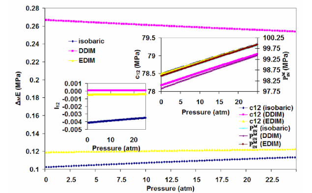
Figure 15: Energy of mixing, mutual cohesive energy density, and correction $l_{12}$ as a function of  pressure for a 50-50 blend. We take $M_{1}=M_{2}=100$, $e_{11}=-2.2\times 10^{-21}$ J, $e_{22}=-2.6\times 10^{-21}$ J, $v_{0}=1.6\times 10^{-28}$ m${}^{\text{3}}$ and $q=14.$ The temperature is fixed at $300^{\circ}$C.

V.5.4 Variation with $T$

We plot $\Delta E_{\text{M}}$ and $l_{12}$ as a function of $T$ in Fig. 16 for isobaric, DDIM, EDIM processes along with the isochoric process. The corresponding $c_{12}$’s, all originating around 90 MPa at $-100^{\circ}$C as a function of $T,$ are shown in Fig. 17. All processes start from the same state at the lowest temperature ($-100^{\circ}$C) in the figure. There is a complicated dependence in $\Delta E_{\text{M}}$ on $T$ over the range considered for some of the processes. Let us first consider the isochoric process in which all quantities show almost no dependence on $T.$ The energy of mixing remains positive in accordance with the London-Berthelot conjecture (10). This is further confirmed by an almost constant $c_{12},$ and an almost vanishing correction $l_{12}$ in the inset. Both isobaric and EDIM processes give rise to negative $\Delta E_{\text{M}},$ thereby violating the London-Berthelot conjecture. The DDIM $\Delta E_{\text{M}}$ shows a peak, which is about eight times in magnitude than its value at the lowest temperature, but remains positive throughout. The corresponding $c_{12}$ shows a continuous decrease to zero with temperature for isobaric, DDIM, and EDIM processes. However, it is almost a constant for the isochoric process. The non-monotonic behavior in temperature of $\Delta E_{\text{M}}$ is correlated with a similar behavior in $l_{12}.$ This behavior is further studied in the next section. From Fig. 16, we observe that $l_{12}$ provides a small correction at $300^{\circ}$C. However, at much higher temperatures, it is no longer a small quantity, and depends strongly on the way the mixture is prepared, even if it remains isometric. In particular, isobaric $l_{12}$ seems to provide the biggest correction. It is almost constant and insignificant for the isochoric and EDIM processes.

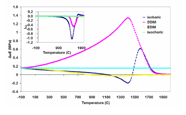
Figure 16: Energy of mixing, mutual cohesive energy density, and correction $l_{12}$ as a function of  temperature for a 50-50 blend. We take $M_{1}=M_{2}=100$, $e_{11}=-2.2\times 10^{-21}$ J, $e_{22}=-2.6\times 10^{-21}$ J, $v_{0}=1.6\times 10^{-28}$ m${}^{\text{3}}$ and $q=14.$ The pressure is fixed at $1.0$ atm.

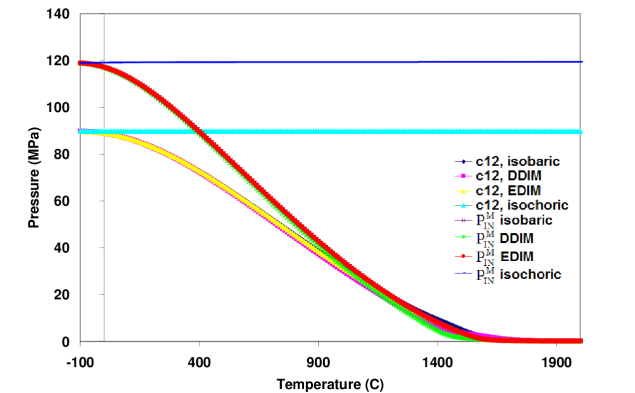
Figure 17: Different mutual pressures as a function of temperature; system as described in Fig. 16.

V.6 Using Internal Pressure

We now introduce a new quantity as another measure of the mutual cohesive pressure by using the internal pressure. To this end, we consider the internal pressure $P_{\text{IN}}$ in the RMA limit. We find from (22a) that

$$P_{\text{IN}}v_{0}\ ^{\underrightarrow{\text{RMA}}}\ q[-e_{11}\phi_{\text{m}1}^{2}/2-e_{22}\phi_{\text{m}1}^{2}/2-e_{12}\phi_{\text{m}1}\phi_{\text{m}2}],$$

which can be expressed as

$$P_{\text{IN}}v_{0}\ {}^{\underrightarrow{\text{RMA}}}\ c_{11}^{\text{P}}x^{2}\phi_{\text{m}}^{2}/\phi_{\text{m}1}^{\text{P}2}+c_{22}^{\text{P}}(1-x)^{2}\phi_{\text{m}}^{2}/\phi_{\text{m}2}^{\text{P}2}+2c_{12}x(1-x),$$

where we have used (39) in the RMA limit. Now we take this equation as a guide to define a new mutual cohesive energy density, the mutual internal pressure $P_{\text{IN}}^{\text{M}}$ in the general case as

$$P_{\text{IN}}^{\text{M}}=[P_{\text{IN}}-c_{11}^{\text{P}}x^{2}\phi_{\text{m}}^{2}/\phi_{\text{m}1}^{\text{P}2}-c_{22}^{\text{P}}(1-x)^{2}\phi_{\text{m}}^{2}/\phi_{\text{m}2}^{\text{P}2}]/2x(1-x).$$

In the RMA limit, $P_{\text{IN}}^{\text{M}}$ reduces to the RMA $c_{12}$ given in (39). We show $P_{\text{IN}}^{\text{M}}$ in the inset in Figs. 13, 15, and 17. What we discover is that isochoric $P_{\text{IN}}^{\text{M}}$ is almost a constant as a function of temperature around 120 MPa, and is larger than isochoric $c_{12},$ which is around 90 MPa. Indeed, over most of the temperatures at the lower end, we find that $P_{\text{IN}}^{\text{M}}$ $>$ $c_{12}$. However, the main conclusion is that both $c_{12}$ and $P_{\text{IN}}^{\text{M}}$ are monotonic decreasing or are almost constant, and behave identically except for their magnitudes.

VI New Approach using SRS: Self-Interacting Reference State

Unfortunately, the van Laar-Hildebrand cohesive energy $c_{12}$ does not have the required property of vanishing with $e_{12},$ see (39). The unwanted behavior of $c_{12}$ is due its definition in terms of the energy of mixing from which we need to subtract pure component (for which $e_{12}$ may be thought to be zero) cohesive energies $c_{ii}^{\text{P}}.$ The subtracted quantity is used to define $c_{12},$ and if this definition has to have any physical significance, it should vanish in the hypothetical state, which we have earlier labelled SRS, in which $e_{12}$ vanishes even though $e_{11}$ and $e_{22}$ are non-zero. The hypothetical state obviously violates the London condition (11), even though the real mixture does not. Let us demand the subtracted quantity to vanish for SRS. To appreciate this point, consider (37) for SRS. It is clear that $\Delta E_{\text{M}}$ continues to depend on the thermodynamic state of the mixture via $\phi_{ii};$ this quantity in general will not be equal to pure component quantity $\phi_{ii}^{\text{P}}$. With the use of (38) in (37), we find that

$$\Delta E_{\text{M}}^{\text{SRS}}v_{0}=e_{11}[\phi_{11}-x\phi_{\text{m}}\phi_{11}^{\text{P}}/\phi_{\text{m}1}^{\text{P}}]+e_{22}[\phi_{22}-(1-x)\phi_{\text{m}}\phi_{22}^{\text{P}}/\phi_{\text{m}2}^{\text{P}}],$$ (47)

which is usually going to depend on the process of mixing. On the other hand, from (35), we observe that

$$\Delta E_{\text{M}}^{\text{SRS}}\overset{c_{12}=0}{=}(c_{11}^{\text{P}}+c_{22}^{\text{P}})\varphi_{1}\varphi_{2},$$ (48)

had $c_{12}=0.$ In this case, $\Delta E_{\text{M}}$ would depend only on pure component quantities $c_{ii}^{\text{P}},$ and its behavior in a given process at fixed composition should be controlled by the behavior of $c_{ii}^{\text{P}}$ in that process. This is not the case, as can be seen in Fig. 18, where we plot $\Delta E_{\text{M}}$ for the hypothetical state SRS for a 50-50 mixture. We have ensured that the SRS state at the initial temperature in Fig. 18 is the same in isobaric and isochoric processes. But the pure components are slightly different. A new process is also considered in Fig. 18, in which we set the volume $V_{\text{SRS}}$ of the hypothetical SRS at a given temperature to be equal to the volume $V$ of the real mixture (nonzero $e_{12}$) at $1.0$ atm at that temperature. This process is labelled isobaric ($V_{\text{SRS}}=$ $V$) in the figure. The pure components are also at $1.0$ atm for this process. Since the pure components for this process are the same as in the isobaric calculation, (48) requires $\Delta E_{\text{M}}$ for the two processes  to be identical at all temperatures. This is evidently not the case. Consider Fig. 11. From this, we see that $c_{ii}^{\text{P}}$ are almost constant with $T$ for the isochoric case. Thus, according to (48), $\Delta E_{\text{M}}$ should be almost a constant, which is not the case. For the isobaric case, $c_{ii}^{\text{P}}$ are monotonic decreasing with $T$, which will then make $\Delta E_{\text{M}}$, according to (48), monotonic decreasing with $T$, which is also not the case. Hence, we conclude that the van Laar-Hildebrand $c_{12}$ does not vanish for SRS.

A similar unwanted feature is also present in the behavior of $P_{\text{IN}}^{\text{M}}$ introduced above for the same reason: it also does not vanish for SRS.

It is disconcerting that the van Laar-Hildebrand $c_{12}(e_{12}=0)$ does not vanish for SRS, even though the mutual interaction energy $e_{12}=0.$ This behavior is not hard to understand. The mixture energy is controlled by the process of mixing, since the mixture state varies with the process of mixing even at $e_{12}$=0.

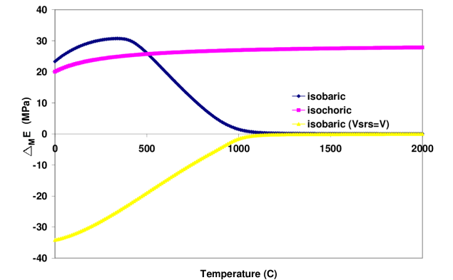
Figure 18: $\Delta E_{\text{M}}$ for IRS as a function of  temperature for a 50-50 blend. We take $M_{1}=M_{2}=100$, $e_{11}=-2.2\times 10^{-21}$ J, $e_{22}=-2.6\times 10^{-21}$ J $v_{0}=1.6\times 10^{-28}$ m${}^{\text{3}}$ and $q=10.$ The pressure is fixed at $1.0$ atm.

VI.1 Mutual Energy of Interaction $c_{12}^{\text{SRS}}$

To overcome this shortcoming, we introduce a new measure of the cohesive energy that has the desired property of vanishing with $e_{12}.$ Let $E$ denote the energy per unit volume of the mixture. We will follow RaneGuj2005 , and compare it with that of the hypothetical reference state SRS. Its energy per unit volume $E_{\text{SRS}}$ differs from $E$ due to the absence of the mutual interaction between the two components. Let $V_{\text{SRS}}$ denote the volume of the SRS. In general, we have

$$V_{\text{SRS}}/V=\phi_{\text{m}}/\phi_{\text{m,SRS}}.$$

The difference

$$E_{\text{int}}^{(\text{M})}\equiv E-(V_{\text{SRS}}/V)E_{\text{SRS}}$$

represents the mutual energy of interaction per unit volume due to $1$-$2$ contacts. From (20), we obtain

$$E_{\text{int}}^{(\text{M})}v_{0}\equiv e_{11}[\phi_{11}-(V_{\text{SRS}}/V)\phi_{11,\text{SRS}}]+e_{22}[\phi_{22}-(V_{\text{SRS}}/V)\phi_{22,\text{SRS}}]+e_{12}\phi_{12},$$

where the contact densities $\phi_{ij}$ without SRS are for the mixture state and with SRS are for the SRS state. These densities are evidently different in the two states but approach each other as $e_{12}\rightarrow 0$. The above excess energy should determine the mutual cohesive energy density, which we will denote by $c_{12}^{\text{SRS}}$ in the following to differentiate it with the van Laar-Hildebrand cohesive energy density $c_{12}$. It should be evident that $E_{\text{int}}^{\text{M}}\$vanishes as $e_{12}$ vanishes due to its definition.

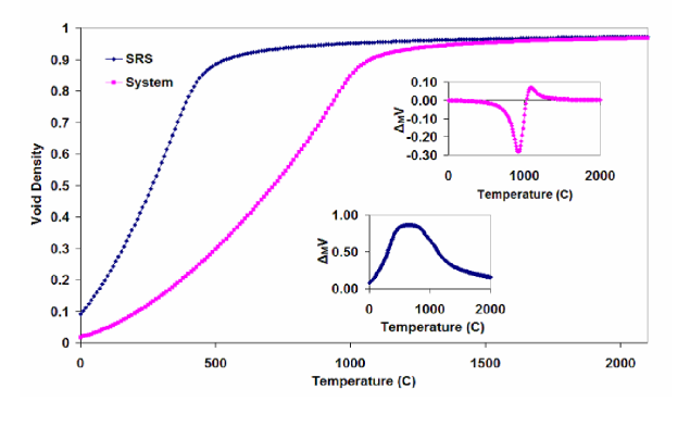
Figure 19: Void density and volume of mixing as a function of  temperature for a 50-50 blend. We take $M_{1}=M_{2}=100$, $e_{11}=-2.2\times 10^{-21}$ J, $e_{22}=-2.6\times 10^{-21}$ J, $v_{0}=1.6\times 10^{-28}$ m${}^{\text{3}}$ and $q=10.$ The pressure is fixed at $1.0$ atm.

The absence of mutual interaction in SRS compared to the mixture causes SRS volume to expand relative to the mixture. This is shown in Fig. 19 in which the void density in SRS is larger than that in the mixture. The relative volume of mixing at constant pressure ($1.0$ atm) for the mixture is shown in the upper inset, and that for SRS is shown in the lower inset. It is clear that the latter relative volume of mixing is always positive, indicating an effective repulsion between the two components. This should come as no surprise since the excess interaction $\varepsilon_{12}$ for SRS from (6)

$$\varepsilon_{12}^{\text{SRS}}=-(e_{11}+e_{22})/2>0,$$

and has the value $2.4\times 10^{-21}$ J in this case. Thus, it represents a much stronger mutual repulsion than the mutual repulsion due to $\varepsilon_{12}\cong 0.1\times 10^{-21}$ J in the mixture. The effect of adding the mutual interaction $e_{12}$ to SRS is to add mutual ”attraction” that results in cohesion, and in the reduction of volume. Thus, the change in the volume can also be taken as a measure of cohesion, as we will discuss below.

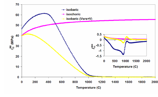
Figure 20: Mutual cohesive energy density, and correction $l_{12}$ using the IRS as a function of  temperature for a 50-50 blend. We take $M_{1}=M_{2}=100$, $e_{11}=-2.2\times 10^{-21}$ J, $e_{22}=-2.6\times 10^{-21}$ J $v_{0}=1.6\times 10^{-28}$ m${}^{\text{3}}$ and $q=10.$ The pressure is fixed at $1.0$ atm.

VI.1.1 RMA Limit of $E_{\text{int}}^{(\text{M})}$

In the RMA limit, along with the monomer equality assumption (40), which implies that $\phi_{\text{m}}=\phi_{\text{m,SRS}},$ it is easily seen that

$$E_{\text{int}}^{(\text{M})}v_{0}{}^{\underrightarrow{\text{RMA}}}qe_{12}\phi_{\text{m}1}\phi_{\text{m}2}=qe_{12}\phi_{\text{m}1}^{\text{P}}\phi_{\text{m}2}^{\text{P}}x(1-x).$$

As a consequence, $E_{\text{int}}^{(\text{M})}/2x(1-x)$ reduces to the RMA value of $(-c_{12})$ given in (39). This means that the quantity $c_{12}^{\text{SRS}}$ defined via

$$c_{12}^{\text{SRS}}\equiv-E_{\text{int}}^{(\text{M})}/2\varphi_{1}\varphi_{2}$$ (49)

has the required property that it not only reduces to the correct RMA value of the van Laar-Hildebrand$\ c_{12},$ but it also vanishes with $e_{12}$. [As usual, we assume the identification (41).]

VI.1.2 New Mutual Cohesive Energy Density: $c_{12}^{\text{SRS}}$

We now take (49) as the general definition of a more suitable quantity to play the role of cohesive energy density. This quantity is a true measure of the effect produced by mutual interaction energy, and which also vanishes with $e_{12}.$ Away from the RMA limit, $c_{12}$ and $c_{12}^{\text{SRS}}$ are not going to be the same. It is evident that $c_{12}^{\text{SRS}}$ depends not only on $T,P,$ or $T,V,$ but also on the composition $x\equiv\phi_{\text{m}1}/\phi_{\text{m}},$ $q$, and the energies $e_{ij}.$ For isochoric calculations, we will ensure that the mixture and SRS have the same monomer density $\phi_{\text{m}}.$ In this case, $V_{\text{SRS}}=V.$ For isobaric calculations, we will, as usual, ensure that they have the same pressure, so that the two volumes need not be the same. However, we will also consider $V_{\text{SRS}}=V$ for isobaric calculations to see the effect of this on $c_{12}^{\text{SRS}}.$ This process is what we have labelled isobaric ($V_{\text{SRS}}=$ $V$) in the Fig. 18. We show $c_{12}^{\text{SRS}}$ for various processes in Fig. 20. We see that it continues to increase monotonically for the isochoric case, and reaches an asymptotic value of about 50 MPa, while van Laar-Hildebrand $c_{12}$ in Fig. 16 is almost constant and about 90 MPa. An increase in solubility with temperature at constant volume is captured by $c_{12}^{\text{SRS}}$ but not by $c_{12}.$ The behavior of the two quantities for the isobaric case is also profoundly different. While $c_{12}$ monotonically decreases with temperature, $c_{12}^{\text{SRS}}$ is most certainly not monotonic. It goes through a maximum around $400{{}^{o}}$C before continuing to decrease. This suggests that the solubility increases before decreasing. This should come as no surprise as we explain later in the following section.

Note that while the definition of $c_{12}^{\text{SRS}}$ is independent of any approximate theory, the definition of $c_{12}$ depends on a form (35) whose validity is of questionable origin as it depends on RST. It should be noted that the value of $c_{12}^{\text{SRS}}$ truly represents the energy change that occurs (in SRS) due to the presence of the mutual interaction between the two components. The changes brought about due to $e_{12}\neq 0$ should not be confused with the changes that occur when the two pure components are mixed ( $e_{12}\neq 0),$ because the latter involves not only the process of mixing when $e_{12}=0$ (this gives rise to SRS ) but also involves the rearrangements of the two components due to the mutual interaction. It is the latter rearrangement due to mutual interaction that determines $c_{12}^{\text{SRS}}.$ This is easily appreciated by studying the void density profiles for SRS and the mixture in Fig. 19. As usual, $e_{12}$ for the mixture is defined by (11). The hypothetical process of mixing (under the condition $e_{12}=0$) also contributes to the energy of mixing, since the energy of this state is not the same as the sum of the two pure systems’ energies, because SRS is affected by mixing the pure components. This is easily seen by computing the energy of mixing $\Delta E_{\text{M,SRS}}$ for SRS for which $e_{12}=0$ but not $e_{11},e_{22}$:

$$V_{\text{SRS}}\Delta E_{\text{M,SRS}}\equiv V_{\text{SRS}}E_{\text{SRS}}-V_{1}^{\text{P}}E_{1}^{\text{P}}-V_{2}^{\text{P}}E_{2}^{\text{P}},$$

where $V_{i}^{\text{P}},E_{i}^{\text{P}}$ are the volume and energy density of the pure $i$th component. This part determines the energy of mixing due to pure mixing at $e_{12}=0,$ and but it has nothing to do with the mutual interaction $e_{12}.$ Thus, this contribution should not be allowed to determine in part the mutual cohesive energy density. It is easy to see that

$$\Delta E_{\text{M}}\equiv E_{\text{int}}^{\text{M}}+(V_{\text{SRS}}/V)\Delta E_{\text{M,SRS}},$$

in which the second contribution is not a true measure of the mutual interaction. Nevertheless, it is considered a part of the van Laar-Hildebrand cohesive energy density. Using (35) and (49) in the above equation, we find that we can express $c_{12}^{\text{SRS}}$ in terms of the van Laar-Hildebrand cohesive energy densities as follows:

$$c_{12}^{\text{SRS}}(e_{12})=c_{12}(e_{12})-c_{12}(e_{12}=0)+(1-\phi_{\text{m}}/\phi_{\text{m,SRS}})(c_{11}^{\text{P}}+c_{22}^{\text{P}})/2.$$ (50)

Here, $c_{12}^{\text{SRS}}(e_{12})$ is the SRS-based $c_{12}^{\text{SRS}}$ introduced in (49), and $c_{12}(e_{12})$ is energy-of-mixing based $c_{12}$ in (35). In the special case $\phi_{\text{m}}=\phi_{\text{m,SRS}},$ the last term vanishes, and the SRS-$c_{12}$ is the difference of the van Laar-Hildebrand-$c_{12}.$ In any case, because of the above relation, studying van Laar-Hildebrand-$c_{12}$ also allows us to learn about the SRS-$c_{12}.$ Therefore, we have mostly investigate $c_{12}$ in the present work. However, it should be realized that we also need van Laar-Hildebrand-$c_{12}$ for SRS, data for which ate not available.

The arguments similar to the presented above suggest that we can similarly use the difference $P_{\text{int}}-$ $P_{\text{int,SRS}},$ where $P_{\text{int,SRS}}$ is the interaction pressure in SRS at the same volume $V$, as a measure of the cohesive pressure for the system. Alternatively, we can use SRS at the same pressure $P$ as the mixture, whose volume $V_{\text{SRS}}$ is different from $V$. We can use the negative of the difference $V-V_{\text{SRS}}$ as a measure for cohesion. However, we will study these quantities elsewhere and not here.

VI.2 Cohesion and Volume

We have argued above that the changes in the volume can also be taken as a measure of cohesion. We now follow this line of thought. The volume of mixing is governed by two factors, as discussed elsewhere Gujrati1998 ; Gujrati2003 : (i) the size disparity between the two components, and (ii) the interactions. To disentangle the two contributions, we can consider the difference

$$\Delta_{\text{ath}}V\equiv V-V_{\text{ath}},$$

where $V_{\text{ath}}$ is the volume of the athermal system (no interaction) at the same $T,P$. (In the athermal limit, $\Delta V_{\text{M,ath}}=V_{\text{ath}}$ $-V_{1}^{\text{P}}-V_{2}^{\text{P}}$ will be identically zero if the two polymer components have identical sizes $\left(M_{1}=M_{2}\right)$, and will be negative if they are different.) The difference $\Delta_{\text{ath}}V$ is governed only by the presence of interactions ($e_{11},e_{22},$ and $e_{12}$). A positive $\Delta_{\text{ath}}V$ will imply an effective repulsion, and a negative $\Delta_{\text{ath}}V$ will imply an effective attraction. Thus, $\Delta_{\text{ath}}V$ can also be used as a measure of the cohesiveness of the mixture.

It is easy to see that

$$V_{\text{ath}}/V=\phi_{\text{m}}/\phi_{\text{m,ath}}=(1-\phi_{\text{0}})/(1-\phi_{\text{0,ath}}),$$ (51)

in terms of total monomer density or void density. Using this, we can also calculate the difference $\Delta_{\text{ath}}v\equiv\Delta_{\text{ath}}V/V$ per unit volume in our theory, and is shown in Fig. 21 in an isobaric process at $1.0$ atm. We note that $\varepsilon_{01}=\varepsilon_{02}=\varepsilon_{12}=0$ ($e_{11}=e_{12}=e_{22}=0$) for the athermal state, while $\varepsilon_{01}=1.1\times 10^{-21}$ J, $\varepsilon_{02}=1.3\times 10^{-21}$ J, and $\varepsilon_{12}\simeq 0.01\times 10^{-21}$ J ($e_{11}=-2.2\times 10^{-21}$J, $e_{12}=-2.6\times 10^{-21}$J$,e_{12}\simeq-2.39\times 10^{-21}$ J) for the mixture. Recall that we have decided to define $e_{12}$ for the mixture by (11). The difference $\Delta_{\text{ath}}v$ is obviously controlled by all three energies $e_{ij}$, and not just by $e_{12}.$ Since the mixture has attractive interactions ($e_{ij}<0$), its volume $V$ is smaller than $V_{\text{ath}}$ so that $\Delta_{\text{ath}}v<0$ as seen in Fig. 21.

To determine the effect of only $e_{12},$ we use SRS in place of the athermal state and introduce the difference

$$\Delta_{\text{SRS}}v=1-(V_{\text{SRS}}/V),$$

which is also shown in Fig. 21. Here, the mixture is compared with the SRS state in which $\varepsilon_{01}=1.1\times 10^{-21}$ J, $\varepsilon_{02}=1.3\times 10^{-21}$ J, but $\varepsilon_{12}=2.4\times 10^{-21}$ J ($e_{11}=-2.2\times 10^{-21}$J, $e_{12}=-2.6\times 10^{-21}$J, $e_{12}=0$). Since the mixture has extra attractive interaction ($e_{12}<0$) than the SRS state ($e_{12}=0$), $V$ is smaller than $V_{\text{SRS}},$ so that the negative value of $\Delta_{\text{SRS}}v$ should not be a surprise. The minimum in $\Delta_{\text{SRS}}v$ is due to the behavior of the void density, which is shown in Fig. 19 for SRS and the mixture. In the two insets, we also show the relative volume of mixing at constant pressure (1.0 atm) for SRS (lower inset) and the mixture (upper inset). We notice that below around $500{{}^{\circ}}$C, the free volume in SRS changes faster than in the mixture, while above it, the converse is the case. This changeover in the rate of change causes the dip and the minimum in $\Delta_{\text{SRS}}v.$ Similarly, the dip in $\Delta_{\text{ath}}v$ is caused by the changeover in the rate of change of free volume in the mixture and the athermal state.

The minimum in $\Delta_{\text{SRS}}v$, see Fig. 21, also explains the intermediate maximum in the isobaric $c_{12}^{\text{SRS}}$ in Fig. 20. The behavior of $c_{12}^{\text{SRS}}$ shows that the mutual cohesiveness increases and then decreases with the temperature, and is merely a reflection of the way the void densities in Fig. 19 behave with the temperature.

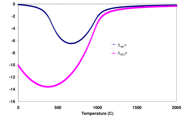
Figure 21: Volume difference $\Delta_{\text{ath}}v$ and $\Delta_{\text{SIRS}}v$ for a 50-50 blend as a function of temperature. We have $M_{1}=M_{2}=100$, $e_{11}=-2.2\times 10^{-21}$ J, $e_{22}=-2.6\times 10^{-21}$ J $v_{0}=1.6\times 10^{-28}$ m${}^{\text{3}}$ and $q=10.$ The pressure is fixed at $1.0$ atm.

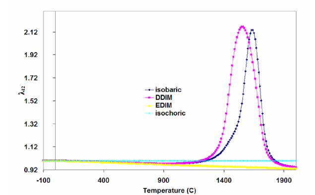
Figure 22: The scaled quantity $\gamma_{12}$ for various processes. This quantity is very close to $1$ except at high temperatures where one of the components seems to be near its boiling. For the system considered, we have $M_{1}=M_{2}=100$, $e_{11}=-2.2\times 10^{-21}$ J, $e_{22}=-2.6\times 10^{-21}$ J $v_{0}=1.6\times 10^{-28}$ m${}^{\text{3}}$ and $q=14.$ The pressure is fixed at $1.0$ atm.

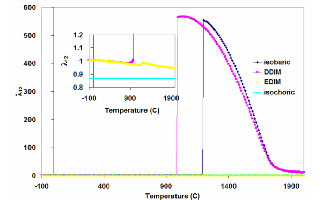
Figure 23: The scaled quantity $\gamma_{12}$ for various processes for a $50-50$ mixture. This quantity is very close to $1$ except at high temperatures where the sharp discontinuity is due to one of its components undergoing boiling. The system is $M_{1}=100,$ $M_{2}=10$, $e_{11}=-2.6\times 10^{-21}$ J$=$ $e_{22},$ $v_{0}=1.6\times 10^{-28}$ m${}^{\text{3}}$ and $q=14.$ The pressure is fixed at $1.0$ atm.

VII More Numerical Results: $\gamma_{12}$ and $l_{12}$

We observe from (39) that the quantity

$$\text{ }c_{12}v_{0}/(-qe_{12}\phi_{\text{m}}^{2}/2)$$

approaches $1$ in the RMA limit. As we have seen earlier (compare Figs. 9 and 10), the quantity $q/2$ in the RMA limit should be properly replaced by ($q/2-\nu)$ for finite $q.$ The new factor incorporates the correction due to end groups. Therefore, we introduce a new dimensionless quantity

$$\gamma_{12}\equiv-c_{12}v_{0}/(q/2-\nu)e_{12}\phi_{\text{m}}^{2},$$

and investigate how close it is to $1.$ Any deviation is due to nonrandom mixing and will provide a clue to its importance. In Fig. 22, we plot $\gamma_{12}$ as a function of temperature for various processes. The coordination number is taken to be $q=14$, and the initial void density is $\phi_{0}=0.00031333.$ This system is identical to the one studied in Fig. 16. For the isochoric process, $\gamma_{12}$ is almost a constant and very close to (but below) $1.$ It decreases gradually for EDIM and becomes almost 0.92 at about $t_{\text{C}}=2000^{\circ}$C. The situation is very different for isobaric and DDIM processes where $\gamma_{12}$ shows enhancement at a temperature near the boiling of one of the pure components. To be convinced that the peak in $\gamma_{12}$ in Fig. 22 is indeed due to boiling, we plot it for $q=14$ in Fig. 23. We see a discontinuity in $\gamma_{12}$ for all cases except for isochoric case, as is evident from the inset (in which isobaric results are not shown). The discontinuity is due to the boiling transition which occurs at different temperatures for the different cases. These discontinuities become rounded as in Fig. 22, when we are close to boiling transitions.

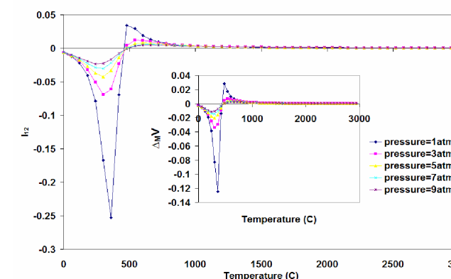
Figure 24: Binary deviation $l_{12\text{ }}$ and the relative volume of mixing in the inset for a $50-50$ mixture. For the system considered, we have $M_{1}=M_{2}=100$, $e_{11}=-2.2\times 10^{-21}$ J, $e_{22}=-2.6\times 10^{-21}$ J $v_{0}=1.6\times 10^{-28}$ m${}^{\text{3}}$ and $q=6.$

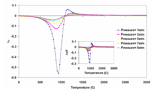
Figure 25: Binary deviation $l_{12\text{ }}$ and the relative volume of mixing in the inset for a $50-50$ mixture. The system considered has $M_{1}=M_{2}=100$, $e_{11}=-2.2\times 10^{-21}$ J, $e_{22}=-2.6\times 10^{-21}$ J, $v_{0}=1.6\times 10^{-28}$ m${}^{\text{3}}$ and $q=14.$

We now turn our attention to the binary correction $l_{12},$ which measures the deviation from the London-Berthelot conjecture (10). The existence of this deviation in the case when we choose $e_{12\text{ }}$ to satisfy the London conjecture (11) will suggest that it is caused by thermodynamics which makes cohesive energies different from their respective van der Walls energies $e_{ij}$. Moreover, the behavior of $l_{12}$ also reflects partially the behavior of the pure components, since the definition of $l_{12}$ utilizes the pure component cohesive energies, see (12), even if $c_{12}$ is defined without any association with them as is the case with $c_{12}^{\text{SRS}},$ whose definition is independent of pure component quantities $c_{ii}^{\text{P}}$. Consider the inset in Fig. 14, which shows $l_{12}$ associated with $c_{12}.$ We observe that it is almost constant for the two cases (DDIM and EDIM) for which mixing is isometric. However, it has a strong variation for the isobaric case where mixing is not isometric. Thus, we see the first hint of a dependence on volume of mixing in the behavior of $l_{12}.$ Such a dependence on the volume of mixing is also seen in the inset showing $l_{12}$ (corresponding to $c_{12})$ in Fig. 16. We are struck by the presence of maxima and minima for the two isochoric cases. They appear to be almost at same temperatures in both cases; notice the location of minima and maxima in the isobaric $l_{12}$ and the volume of mixing.

To further illustrate the relationship between isobaric $l_{12}$ and the volume of mixing $\Delta v_{\text{M}}$, we plot them as a function of the temperature in Figs. 24 and 25 for $q=6$ and $q=14,$ respectively, for several values of the pressure $P.$ The strong correlation between their maxima and minima are clearly evident. These figures illustrate that the binary correction $l_{12}$ for the isobaric process closely follows how the volume of mixing $\Delta v_{\text{M}}$ behaves. A negative $\Delta v_{\text{M}}$ is a consequence of the effective attraction between the mixing components, which corresponds to a larger value of their mutual cohesive energy density $c_{12}$; this is reflected in a corresponding negative value of $l_{12}.$ As the pressure increases, the correction decreases and the system gets closer to satisfying the the London-Berthelot conjecture (10). Thus, we can conclude that the binary correction is negligible, but not zero, as long as the volume of mixing is very small or even zero.

VIII Discussion and Conclusions

We have carried out a comprehensive investigation of the classical concept of cohesiveness as applied to a thermodynamic system composed of linear polymers. In pure components, we are only dealing with one kind of interaction: microscopic self-interactions between the monomers. Therefore, we are interested in relating this microscopic self-interaction to a thermodynamic quantity in order to estimate the strength of the microscopic self-interaction. In binary mixtures (polymer solutions or blends), there are two self interactions, and one mutual interaction. The microscopic self interactions in the mixture do not depend on the state of the mixture. Therefore, they are evidently the same as in pure components. Thus, it is the microscopic mutual interaction that is new, and needs to be extracted by physical measurements. However, what one measures experimentally is not the microscopic interaction strengths, but macroscopic interaction strengths due to thermodynamic modifications.

Traditionally, cohesive energies have been used as indicators of the macroscopic interaction strengths. The definition of $c^{\text{P}}$ for pure components, given in (2), does not depend on any particular approximation or any theory. It is a general definition. Thus, it can be measured directly if the interaction energy $\mathcal{E}_{\text{int}}$ can be measured. It can also be calculated by the use of any theory. Only the obtained value will depend on the nature of the theory.

On the other hand, the mutual cohesive energy density $c_{12}$ is defined by a particular form of the energy of mixing. This gives rise to two serious limitations of the definition. The first deficiency is caused by the use of the form (35), whose validity is questionable. Thus, the extracted value of $c_{12}$ is based on this questionable form. The second deficiency is that this value also depends on pure component properties $c_{ii}^{\text{P}},$ since the mutual energy is measured with respect to the pure components. However, we have argued that the energy of the mixture will be different from the sum of the pure component energies even if $e_{12}$ is absent. Thus, $c_{12}$ does not necessarily measure mutual interactions. One of our aims was to see if some thermodynamic quantity can be identified that could play the role of a true $c_{12}$ that would vanish with $e_{12}.$ This is the quantity $c_{12}^{\text{SRS}}$ that we have identified in this work. There is no such problem for $c^{\text{P}},$ since it not only vanishes with $e$, as we have seen before, but it also does not suffer from any approximation.

We follow our recent work RaneGuj2005 in the approach that we take here. We confine ourselves to a lattice model, since the classical approach taken by van Laar vanLaar and Hildebrand Hildebrand is also based on lattice models in that their theory can only be justified consistently by a lattice model. We then introduce two different reference states to be used for pure components and mixtures, respectively. For pure components, we introduce a hypothetical reference state in which this self-interaction is absent. Since there is only one interaction, which is absent in the reference state, this state is nothing but the athermal state of the pure component. With the use of this state, we introduce the interaction energy $\mathcal{E}_{\text{int}}$ defined via (1). Because of the subtraction in (1), $\mathcal{E}_{\text{int}}$ depends directly on the strength of the self-interaction, the only interaction present in a pure component that we wish to estimate. Thus, it is not a surprise that $\mathcal{E}_{\text{int}}$ is an appropriate thermodynamic quantity that can be used to estimate the strength of the self-interaction. Consequently, we use this quantity to properly define the pure component cohesive energy density $c^{\text{P}}$ at any temperature. We have discussed how this definition resembles the conventional definition of $c^{\text{P}}$ in the literature. For the mixture, we introduce the self-interacting reference state (SRS), which allows us to define $c_{12}^{\text{SRS}}$ that vanishes with $e_{12}.$ In contrast, the van Laar-Hildebrand $c_{12}$ does not share this property.

As noted earlier, our approach allows us to calculate $c^{\text{P}}$ and $c_{12}$ even for macromolecules like polymers, which is of central interest in this work or for polar solvents, which we do not consider here but hope to consider in a separate publication. The cohesive energy density $c^{\text{P}}$ is a macroscopic, i.e. a thermodynamic quantity characterizing microscopic interparticle interactions in a pure component. In general, being a macroscopic quantity, $c^{\text{P}}$ is a function of the lattice coordination number $q$, the degree of polymerization $M$, and the interaction energy $e,$ in addition to the thermodynamic state variables $T,$ and $P$ or $V.$ We have investigated all these dependences in our study here. The same is also true for $c_{12}.$

Based on the same philosophy, we need to introduce another hypothetical reference state called the self-interacting reference state (SRS) for a blend, which differs from a real blend in that the mutual interactions are absent, but self-interactions are the same. The difference $\mathcal{E}_{\text{int}}^{\text{M}}$ introduced in (5) allows us to estimate the strength of the microscopic mutual interaction between the two components of a blend; we denote this estimate by $c_{12}^{\text{SRS}}$ to distinguish it from the customary quantity $c_{12}$ originally due to van Laar, and Hildebrand and coworkers. However, $\mathcal{E}_{\text{int}}^{\text{M}}$ is not what is usually used to define the mutual cohesive energy density $c_{12}.$ Rather, one considers the energy of mixing $\Delta E_{\text{M}}$. We have compared the two approaches in this work.

The conventional van Laar-Hildebrand approach to solubility is based on the use of the regular solution theory. Thus, several of its consequences suffer from the limitations of the regular solution theory (RST). One of the most severe limitations, as discussed in the Introduction, is that the theory treats a solution as if it is incompressible. This is far from the truth for a real system. Hence, one of the aims of this work is to investigate the finite compressibility effects, i.e., the so-called ”equation-of-state” effects. As a real solution most definitely does not obey the regular solution theory, the experimental results usually will not conform to the predictions of the theory. Thus, we have revisited the solubility ideas within the framework of a new theory developed in our group. This theory goes beyond the regular solution theory and also incorporates equation-of-state effects. We have already found that this theory is able to explain various experimental observations, which the regular solution theory (Flory-Huggins theory for polymers) cannot explain. Therefore, we believe that the predictions of this theory are closer to real observations than those of the regular solution theory.

VIII.1 Pure Components

We have first studied the cohesive energy density $c^{\text{P}}$of a pure component. Since it is determined by the energy density of vaporization, it is a quantity independent of the temperature. It is also clear from the discussion of the van der Waals fluid that $c^{\text{P}},$ defined by (2), is independent of the temperature, since the parameter $a$ in (30) is considered $T$-independent. This particular aspect of $c^{\text{P}}$ ensures the equality of $P_{\text{IN}}\equiv-P_{\text{int}}\$and $(\partial\mathcal{E}/\partial V)_{T};$ see (33). For a pure component, Hildebrand Hildebrand1916 has argued that the solubility of a given solute in different solvents is determined by relative magnitudes of internal pressures, at least for nonpolar fluids. Thus, we have also investigated the internal pressure. However, the equality (33) is not valid in general as we have shown above. Thus, the internal pressure, while a reliable and alternative measure of the cohesion of the system in its own right, cannot be equated with $(\partial\mathcal{E}/\partial V)_{T}.$ Their equality is shown to hold only in RMA. If we allow $a$ in (30) to have a temperature-dependence, the equality (33) will no longer remain valid. Moreover, it can be easily checked that under this situation, $P_{\text{IN}}~{}$and $c^{\text{P}}$ for the van der Waals fluid will no longer be the same.

We have investigated the pure component $c^{\text{P}}$ using our recursive theory. We find that it is very different depending on whether we consider an isochoric process, in which case it is almost constant with $T$, or an isobaric process, in which case it gradually decreases to zero at very high $T$. In general, we find that

$$c_{V}^{\text{P}}\ \geq c_{P}^{\text{P}}.$$

We have found that isochoric $c^{\text{P}}$ and $P_{\text{IN}}$ are almost constants as a function of $T.$ It provides a strong argument in support of their usefulness as a suitable candidate for the cohesive pressure. But $c^{\text{P}}$ and $P_{\text{IN}}$ do not remain almost constant in every process, as the isobaric results in Fig. 2 clearly establish. The same figure also shows in its inset that the isobaric $c^{\text{P}}$ exhibits a discontinuity due to boiling, as expected. Unfortunately, most of the experiments are done under isobaric conditions; hence the use of isochoric cohesive quantities may not be useful, and even misleading and care has to be exercised. We also see that $c^{\text{P}}$ changes a lot over the temperature range and replacing it by its value at the boiling point may be not very useful in all cases.

The cohesive energy also depends on the molecular weight, and usually decreases with $M$ as expected; see Fig. 7. This is the situation for $q=14,$ and should be contrasted with the behavior shown in the inset in Fig. 2, where we show $c_{P}^{\text{P}}$ for $M=10,$ and $100,$ but for $q=10.$ All other parameters are the same as in Fig. 7. What we observe is that at low temperatures, $c_{P}^{\text{P}}$ for $M=10$ lies above the $c_{P}^{\text{P}}$ for $M=100,$ while the situation is reversed at high temperatures. This crossover is due to the boiling transition that the smaller $M$ pure component must undergo at about $600{{}^{\circ}}$C. Thus, $c_{P}^{\text{P}}$ decreases with increasing $M$ only far below the boiling temperatures. The dependence on the lattice coordination number $q$ is also not surprising: it increases with $q$ but requires end group correction in that $c^{\text{P}}$ is proportional to $(q/2-\nu);$ see Fig. 9. This means that the solubility function $\delta$ also depends on the process, and its value at the boiling temperature of the system will be dramatically different in the two processes. We have also found, see Fig. 6, that $c^{\text{P}}$ is not truly a quadratic function of the monomer density, one of the predictions of the regular solution theory.

VIII.2 Mixtures (Solutions or Blends)

We now turn to the mutual cohesive energy density $c_{12}.$ Here, the situation is muddled since the definition of $c_{12}$ is based on a form (35) of the energy of mixing $\Delta E_{\text{M}},$ whose validity is questionable beyond RST. This should be contrasted with the definition of $c^{\text{P}},$defined by (2), which is independent of any particular theory. Therefore, $c^{\text{P}}$ can be calculated in any theory without any further approximation except those inherent in the theory. It can also be measured directly by measuring $\mathcal{E}_{\text{int}},$ and does not require any further approximation to extract it. On the other hand, the calculation of $c_{12}$ in any theory requires calculating $\Delta E_{\text{M}}$ in that theory; thus, this calculation is based on the approximations inherent in the theory. However, one must still extract $c_{12}$ from the calculated $\Delta E_{\text{M}}$ by expressing $\Delta E_{\text{M}}$ in the form (35). As discussed above, this form is justified only in RST and $c_{12}$ in (35) at this level of the approximation is indeed a direct measure of the mutual interaction energy $e_{12}.$ Whether $c_{12}$ defined by the form (35) still has a direct dependence on $e_{12}$ is one of the questions we have investigated here by introducing SRS. For $c_{12}$ to be a direct measure of the mutual interaction energy $e_{12},$ we have to ensure that it vanish in SRS. What we have shown is that $c_{12}$ does not vanish in SRS as seen in Fig. 18. A new measure of the mutual cohesive energy density $c_{12}^{\text{SRS}}$ is introduced in (49), which has the desired property.

The reference state SRS behaves very different from the mixture or its athermal analog, as clearly seen from the Figs. 18,19, and 21. In particular, SRS has strong repulsive interactions between the two species. This results in the SRS volume to be much larger than that of the mixture. Therefore, it is possible that the two components may undergo phase separation in SRS. Its use to define $c_{12}^{\text{SRS}}$, therefore, should only be limited to the case where SRS is a single phase state so as to compare with the mixture. We do not report any result when SRS is not a single phase.

We have found that $c_{12}^{\text{SRS}}$ has the correct behavior that it first rises and then decreases with $T$ for a compressible blend. As explained above, this is a reflection of the way the void density behaves with the temperature, as shown in Fig. 21. The rise and fall of cohesion is not apparent in the temperature-dependence of $c_{12}$. It has also been shown that $c_{12}^{\text{SRS}}$ can be expressed in terms of $c_{12}.$ Therefore, we have basically explored the behavior of $c_{12}$ more than that of $c_{12}^{\text{SRS}}.$ As expected, and as shown in Fig. 12, $c_{12}$ increases with $q.$ However, it is not just simply a linear function of $q$, as seen in Fig. 12. It is also clear from the behavior in this figure that $c_{12}$ changes its curvature with $T.$ Thus, $c_{12}$ is not linear with the inverse temperature $\beta$ over a wide range of temperatures.

We have been specifically interested in the contribution due to volume of mixing. For this reason, we have considered three different kinds of isometric mixing (zero volume of mixing), two of which we have called EDIM and DDIM. These are introduced in Sect. V. The third isometric mixing is studied as part of isochoric processes, which we have also considered. The fourth process is an isobaric process in which mixing is at constant pressure. We have also compared $c_{12}$ with a related internal pressure quantity $P_{\text{IN}}^{\text{M}},$ which is another measure of the mutual cohesive energy density or pressure. For a particular process, the two quantities behave similarly, though their magnitudes are different in that $P_{\text{IN}}^{\text{M}}>c_{12};$ see Fig. 17. We have found that isobaric and EDIM quantities are somewhat similar, and both are different from the DDIM quantities. All three quantities have a strong temperature dependence, but the isochoric quantity is very different in that $c_{12}$ or $P_{\text{IN}}^{\text{M}}$ for the latter remains almost a constant with $T.$

We have paid special attention to the violation of the Scatchard-Hildebrand conjecture (3) even when the microscopic interactions obey the London conjecture (11). We find that even under isometric mixing (EDIM), the energy of mixing can become negative, as seen in Fig. 16. There is another possible source of violation of the Scatchard-Hildebrand conjecture seen in Fig. 13. Here, the pure components in the isobaric and DDIM processes remain the same, so that the pure component solubilities $\delta$ are the same. Therefore, from (3) we would conclude that the energy of mixing should be zero, regardless of the process. What we find is that the energy of mixing is not only not zero, it is also different in the two processes. This violation is due to non-random mixing caused by size and/or interaction strength disparity.

We have also investigated the behavior of the binary correction $l_{12}.$ We find that it need not be small. In particular, we find that it becomes very large in isobaric and DDIM processes as seen in Fig. 16. As the pressure increases, $l_{12}$ decreases in magnitude and the deviation from the London-Berthelot conjecture (10) becomes smaller. This effect shows that the deviation from the London-Berthelot conjecture is due to the presence of compressibility. Thus, the behavior of the free volume determines that of $l_{12}.$ In the isobaric case, we have discovered a very interesting fact. The behavior of $l_{12}$ mimics the behavior of the volume of mixing as seen clearly in Figs. 24, and 25. This observation requires further investigation to see if there is something unusual about isobaric processes or it is jut due to non-isometric mixing in the presence of free volume..

In summary, we have found that it is not only the non-isometric mixing by itself that controls the behavior of the cohesive quantities, but also the non-random contributions.

- (1) J.J. van Laar, Sechs Vorträge über das thermodynamische Potential, Braunschweis (1906); Z. physik. Chem., 72, 723 (1910), and 83, 599 (1913). J.J. van Laar and R. Lorentz, Z. allgem. Chem., 146, 42 (1925).
- (2) J.H. Hildebrand, J. Am. Chem. Soc., 38, 1452 (1916); 41, 1067 (1919).
- (3) J.H. Hildebrand, J.H. Prausnitz and R.L. Scott, Regular and Related Solutions, Van Nostrand Reinhold, New York (1970).
- (4) P. Choi, Macromol Rapid Commun, 23, 484 (2002); L. Zhao and P. Choi, Polymer, 45, 1349 (2004).
- (5) Y.Y. Du, Y. Xue and H.L. Frisch, ”Solubility Parameters,” in Physical Properties of Polymers Handbook, ed. J.E. Mark, American Institute of Physics, Woodbury, New York (1996).
- (6) C.M. Hansen, J. of Paint Tech. 39, 104 (1967).
- (7) P.D. Gujrati, J. Chem. Phys., 112, 4806 (2000).
- (8) P.D. Gujrati, J. Chem. Phys., 108, 6952 (1998).
- (9) P.D. Gujrati, Recent Res. Devel. Macromol., 7, 127 (2003); cond-mat/0308598.
- (10) The Flory-Huggins theory is an example of the isometric RMA theory.
- (11) J. Israelachvili, Intermolecular and Surface Forces, Academic Press, London (1997); p.102.
- (12) B.B. Sauer and G.T. Dee, Macromolecules, 35, 7024 (2002).
- (13) S.S. Rane and P.D. Gujrati, Mol. Phys., 101, 2533 (2003).
- (14) M. Chhajer and P.D. Gujrati, J. Chem. Phys., 109, 9022 (1998).
- (15) P.D. Gujrati, J. Chem. Phys., 112, 4806 (2000). S.S Rane and P.D. Gujrati, Eur. Poly. J. 41,1846 (2005).
- (16) N. Schuld and B.A. Wolf in Polymer Handbook, Eds. J. Brandrup and E.H. Immergut, Wiley Interscience, N.Y. 4th Edition (1999). N. Schuld and B.A. Wolf, J. Poly. Sci. Part B 39, 651 (2001); V.N. Kuleznev, B.A. Wolf, and N.A. Pozharnova, J. Poly. Sci. Part B 44, 67 (2002).
- (17) P.D. Gujrati, Phys. Rev. Lett., 74, 1361 (1995).
- (18) J-H Ryu and P.D. Gujrati, J. Chem. Phys., 107, 3954 (1997).
- (19) P.D. Gujrati, Phys. Rev. Lett., 74, 809 (1995).
- (20) F. Semerianov and P.D. Gujrati, Phys. Rev. E 72, 011102 (2005).
- (21) L.D. Landau and E.M. Lifshitz, Statistical Physics, Part 1, Third Edition, Pergamon Press, Oxford (1986).