Local Strong Coupling Pairing in $D$-Wave Superconductor with Inhomogeneous Bosonic Modes

Abstract

Recent local tunneling data indicate strong nanoscale inhomogeneity of superconducting gap in high temperature superconductors. Strong local nanoscale inhomogeneity in the bosonic scattering mode has also been observed in the same samples. We argue that these two inhomogeneities directly related to each other. To address local boson scattering effects, we develop a local strong coupling model of superconducting pairing in a coarse grained superconducting state. Each patch is characterized by local coupling to the bosonic mode as well as by local mode energy. We find that local gap value on each patch grows with the local strength of electron-boson interaction. At the same time local gap value decreases with the local boson mode energy, an observation consistent with the tunneling experiments. We argue that features in the tunneling spectrum due to boson scattering are consistent with experimentally observed spectra. We also address the ${}^{16}O$ to ${}^{18}O$ isotope substitution. Since both coupling constant and boson energy could change upon isotope substitution, we prove that interplay between these two effects can produce results that are very different from conventional BCS model.

I Introduction

Electron-boson interaction is at the center of the pairing interaction in conventional superconductors. Pioneering work of Eliashberg, Eliashberg:60 McMillan and Rowell, McMillan:65 , and Scalapino Scalapino:69 conclusively proved that the non-BCS features in the tunneling spectra in conventional superconductors are directly related to the electron-boson coupling and ultimately to the formation of the superconducting state. Experimental evidence of the “strong-coupling” features Carbotte:90 in the tunneling spectra was clearly connected to the known phonon spectra in these materials. Giaever:60 On the other hand the number of superconducting materials where electron-boson coupling has been seen was small and initial weak coupling approach of Bardeen-Copper-Schrieffer theory was successful in predicting all the measured properties in these materials. The few superconductor, like Pb and Sn, with clear electron-phonon features in the spectrum were called “bad actors” because of deviations from BCS predictions.

In this paper we will focus on high temperature superconductors (high-$T_{c}$). In high-$T_{c}$ materials situation is very different. Tunneling spectra in all of these materials clearly deviates from the mean field BCS $d$-wave tunneling density of states (DOS), see e.g. Fig.(7). In this sense all of the high-$T_{c}$ materials are “bad actors”.

There has been substantial evidence for strong quasiparticle renormalization from tunneling Huang89 ; Mandrus91 ; Renner95 ; Renner96 ; DeWilde98 ; Yurgens99 ; Zasadzinski00 ; Zasadzinski01 and angle-resolved photoemission (ARPES) Dessau91 ; Ding96 ; Shen93 ; Campuzano99 ; Bogdanov00 ; Kaminski01 ; Lanzara01 ; Johnson01 ; Zhou03 ; Kim03 ; Gromko03 ; Sato03 ; Cuk04 ; Zhou05 experiments. The strong quasiparticle renormalization has been suggested as a manifestation of strong electronic coupling to collective modes. Dahm96 ; Shen97 ; Norman97 ; Norman98 ; Abanov99 ; Eschrig00 ; Norman01 ; Manske01 ; Abanov03 ; Sandvik04 ; Devereaux04 ; Bogdanov00 ; Kaminski01 ; Lanzara01 ; Johnson01 ; Zhou03 ; Kim03 ; Gromko03 ; Sato03 ; Cuk04 ; Zhou05 Observed strong electron-electron correlations are clearly important for mechanism of superconductivity. At the same time the physics of electron-boson coupling in these materials is crucial for understanding of the pairing in these materials. We would argue that these features of the tunneling spectra are due to strong electron-boson coupling.

Recent scanning tunneling microscope (STM) experiments reveal strong electronic inhomogeneity. Cren00 ; Howard01 ; Pan01 ; Lang02 ; Fang04 ; McElroy05 More recent experiments with inelastic electron tunneling spectroscopy (IETS STM) have allowed one to directly observe inelastic tunneling features in Bi₂Sr₂CaCu₂O_8+δ (BSCCO) high-$T_{c}$ materials. These experiments have shown that bosonic modes that produce strong coupling features in tunneling spectra are also inhomogeneous on the scale of $20-50\AA$.Jinho1 Nontrivial correlations between local gaps and local boson mode energies were observed.

Here we follow the notion that deviations from the BCS tunneling DOS in these materials are caused by the strong coupling effects due to electron-boson interaction in these materials. We present a strong coupling theory of $d$-wave superconductor where superconducting state arises as a result of a pairing mediated by bosonic modes, that is attractive in $d$-wave channel.

In this regard, the treatment is analogous to the conventional Eliashberg-McMillan-Rowell approach. The main departure from the conventional approach is that we explicitly allow inhomogeneity in the electron-boson coupling strength and the bosonic mode energy. Typical size of inhomogeneity we will assume is on the order of $20-50\AA$. We will assume that the pairing is local and determined by local values of coupling strength and mode energy at the given patch. This approximation allows us to simplify the calculation dramatically. If one takes guidance from the data, it is clear that inelastic tunneling features and superconducting gaps are rather local, and there is no “self-averaging” seen in the tunneling spectra. In other words, local approximation might be a good starting point for this kind of analysis.

We solve self-consistently the Eliashberg equations on each patch and find local $d$-wave order parameter. Random Gaussian distributions of the local coupling constant and local mode energy are considered. As the result, local order parameter (OP) values are random maps that correlate with the input parameters. We find that the local OP positively correlate with the coupling constants. One of the most important findings of this local formalism is that we find indeed anticorrelation between the typical local boson frequency and the superconducting OP. This negative correlation is a direct consequence of the strong local coupling nature of the pairing we assumed. The IETS-STM experiment by Lee et al. Jinho1 has indeed shown a negative correlation between gaps and IETS mode energy.

Using our local model we also address isotope effect. The most commonly used isotope substitution for high-$T_{c}$ materials is ${}^{16}O$ by ${}^{18}O$ substitution. Isotope effect was studied in the past by measurements other than STM tunneling. Here we point to the important papers in this regard by Shen and Lanzara groups  Lanzara01 that argue how isotope effect can change both the characteristic bosonic frequency and the coupling constant to the local bosonic mode.Bogdanov00 ; Lanzara01 ; Zhou03 ; Cuk04 ; Zhou05 We find that isotope shift in these two quantities can either work together to mutually enhance the superconducting gap, or they can work against each other partially cancelling and therefore making net isotope effect small. Hence we conclude that the naive arguments about the “smallness” of isotope effect with substitution of ${}^{16}O$ by ${}^{18}O$ are misleading.

While in this paper we focus on electron-boson interaction, in real systems this interaction contributes to the pairing in these materials. We would like to make it clear that we believe pairing in high-$T_{c}$ materials is a result of interplay between strong electron-electron correlations Nunner05 and electron-boson interaction. To address the effects of spatial inhomogeneity of tunneling IETS spectra we focus only on electron-boson coupling, ignoring electron-electron interaction part that will not produce IETS features. It is not clear how high the transition temperature would be assuming only electron-boson pairing. We leave this question for a separate investigation.

The outline of the paper is as follows: In Sec. II, we will introduce local strong coupling formalism, and outline the details of the formalism starting with the general inhomogeneous pairing theory in reals space. In Sec. III, we will present results from solving self-consistently the strong coupling equations. In Sec. IV we will discuss the isotope effect for inhomogeneous superconductor. We conclude in Sec. V.

II Local pairing formalism

We start with the strong coupling analysis in the local pairing limit. Locality here would be understood in the sense of a coarse grain approach where we assume that the typical sizes of grains are on the order of the coherence length of superconductor $\xi\sim 20\AA$. This assumption is consistent with the STM observed granularity in Bi2212 . Jinho1 ; McElroy05

We will present a detailed description of local strong coupling theory with the steps in the logic outlined. Some of the points are well known but we keep them in for completeness. The formulas are very similar to the standard Eliashberg discussion except we want to stay with the real space description.  McMillan:65 ; Eliashberg:60 ; Scalapino:69

Taking the STM data as guidance we can imagine that we take a coarse grained vies of the sample. We are taking the given field of view and pixelizing it in a set of boxes with characteristic size of $20\times 20\AA$. Each of the pixels will be assigned three variables: order parameter $W({\bf R})$, bosonic mode energy $\Omega_{0}({\bf R})$ and local coupling constant $g({\bf R})$. Coupling constant and bosonic mode energy variables are randomly drawn from the given distribution. We calculate the local order parameter self-consistently.

To start we write down the Green’s function equations in the Nambu space, assuming no translational invariance. We consider the case of both electron-electron and electron-boson interactions being present. The electron-boson coupling term in the Hamiltonian assuming no translational invariance is:

$$H_{e-lattice}=\int d{\bf r}d{\bf r}^{\prime}d{\bf r}^{\prime\prime}c^{{\dagger}}_{{\bf r}\sigma}c_{{\bf r}^{\prime}\sigma}(b^{{\dagger}}_{{\bf r}^{\prime\prime}}+b_{{\bf r}^{\prime\prime}})g({\bf r},{\bf r}^{\prime},{\bf r}^{\prime\prime})\;,$$ (1)

where $g({\bf r},{\bf r}^{\prime},{\bf r}^{\prime\prime})$ is the coupling constant and $x({\bf r})=b_{\bf r}+b^{\dagger}_{\bf r}$ is the boson field. If we assume that only electronic density coupled to the lattice degrees of freedom, then coupling constant $g({\bf r},{\bf r}^{\prime},{\bf r}^{\prime\prime})=g({\bf r})\delta_{{\bf r},{\bf r}^{\prime}}\delta_{{\bf r},{\bf r}^{\prime\prime}}$. The bosons that couple to the electronic density on the other hand are taken to be on the bonds connecting nearest neighbor sites, or alternatively to reside on the dual lattice. We will focus on the local bosonic mode coupling. This seem to be a general enough situation that we believe will capture the relevant physics to be addressed.

Next we consider the second order terms in the effective action that would look like

$$\int d{{\bf r}{\bf r}^{\prime}{\bf r}^{\prime\prime}}d{{\bf r}_{1}{\bf r}_{1}^{\prime\prime}{\bf r}_{1}^{\prime\prime\prime}}\int_{0}^{\beta}d\tau d\tau_{1}g({\bf r},{\bf r}^{\prime},{\bf r}^{\prime\prime})g({\bf r}_{1},{\bf r}_{1}^{\prime},{\bf r}_{1}^{\prime\prime})c^{{\dagger}}_{{\bf r}\sigma}(\tau)c_{{\bf r}^{\prime}\sigma}(\tau)c^{{\dagger}}_{{\bf r}_{1}\sigma_{1}}(\tau_{1})c_{{\bf r}_{1}^{\prime}\sigma_{1}}(\tau_{1})x_{\mathbf{r^{\prime\prime}}}(\tau)x_{\mathbf{r_{1}^{\prime\prime}}}(\tau_{1})\;,$$ (2)

here we assume that phonon propagator $B({\bf r}-{\bf r}_{1},\tau-\tau_{1})=-\langle T_{\tau}x({\bf r})(\tau)x({\bf r}_{1})(\tau_{1})\rangle$ is local given the STM data that indicate the strong local variations of the bosonic excitations as seen in IETS STM Jinho1 . Thus we assume

$$-\langle T_{\tau}x({\bf r})x({\bf r}_{1})\rangle=B({\bf r},\tau)\delta_{{\bf r},{\bf r}^{\prime}}$$ (3)

Then in the self-energy terms electron-boson interaction would produce the term that we would look as $g({\bf r})g({\bf r}^{\prime\prime\prime})B_{\Omega_{m}}({\bf r},{\bf r}^{\prime}|{\bf r}^{\prime\prime},{\bf r}^{\prime\prime\prime})$. We again stress here that both coupling constant $g$ and boson energy will be assumed inhomogeneous. This situation is qualitatively different from weak coupling approach where only single effective coupling constant will be position dependent.

Equation for Green’s functions in Matsubara frequency $\omega_{n}=\pi(2n+1)k_{B}T$ becomes:

$$\left(\begin{array}[]{cc}{\hat{\varepsilon}}_{\bf r}-S({\bf r},{\bf r}^{\prime},i\omega_{n})&W({\bf r},{\bf r}^{\prime},i\omega_{n})\\ W^{*}({\bf r},{\bf r}^{\prime},i\omega_{n})&-{\hat{\varepsilon}}_{\bf r}-S({\bf r},{\bf r}^{\prime},i\omega_{n})\\ \end{array}\right)\bigotimes{\hat{G}}({\bf r}^{\prime},{\bf r}^{\prime\prime},i\omega_{n})=\mathbf{1}\delta({\bf r}-{\bf r}^{\prime\prime})$$ (6)

with $\bigotimes$ understood as a convolution in real space. ${\hat{\varepsilon}}_{\bf r}$ is the kinetic energy operator, that in momentum space will have the form $\varepsilon({\bf k})=-t(\cos(k_{x}a)+\cos(k_{y}a))-\mu$, $\mu$ being the chemical potential. $\mathbf{1}$ being the indentity matrix,and $\hat{G}({\bf r},{\bf r}^{\prime},i\omega_{n})$ being a matrix in Nambu space with relevant components $\hat{G}({\bf r},{\bf r}^{\prime},i\omega_{n})_{11}=G({\bf r},{\bf r}^{\prime},i\omega_{n})$ and $\hat{G}({\bf r},{\bf r}^{\prime},i\omega_{n})_{12}=F({\bf r},{\bf r}^{\prime},i\omega_{n})$ being the normal and anomalous Green’s functions.

We also explicitly keep the normal self energy in the Gorkov equations: $S({\bf r},{\bf r}^{\prime},i\omega_{n})$ that renormalizes the normal selfenergy propagators.

Normal and anomalous selfenergies are defined selfconsistently through:

$$S({\bf r},{\bf r}^{\prime},i\omega_{n})=-T\sum_{m}\int d{\bf r}^{\prime\prime}d{\bf r}^{\prime\prime\prime}V_{\omega_{n}-\omega_{m}}({\bf r},{\bf r}^{\prime}|{\bf r}^{\prime\prime},{\bf r}^{\prime\prime\prime})G({\bf r}^{\prime\prime},{\bf r}^{\prime\prime\prime},i\omega_{m})$$ (7)

$$W({\bf r},{\bf r}^{\prime},i\omega_{n})=-T\sum_{m}\int d{\bf r}^{\prime\prime}d{\bf r}^{\prime\prime\prime}V_{\omega_{n}-\omega_{m}}({\bf r},{\bf r}^{\prime}|{\bf r}^{\prime\prime},{\bf r}^{\prime\prime\prime})F({\bf r},{\bf r}^{\prime},i\omega_{n})$$ (8)

where the effective pairing interaction $V_{\Omega_{m}}({\bf r},{\bf r}^{\prime}|{\bf r}^{\prime\prime},{\bf r}^{\prime\prime\prime})$ is given by the combination of both direct and lattice-vibration-induced electron-electron interaction:

$$V({\bf r},{\bf r}^{\prime}|{\bf r}^{\prime\prime},{\bf r}^{\prime\prime\prime})_{\Omega_{n}}=V^{ee}({\bf r},{\bf r}^{\prime}|{\bf r}^{\prime\prime},{\bf r}^{\prime\prime\prime})-g({\bf r})g({\bf r}^{\prime\prime\prime})B_{\Omega_{m}}({\bf r},{\bf r}^{\prime}|{\bf r}^{\prime\prime},{\bf r}^{\prime\prime\prime})$$ (9)

$V$ is defined on Matsubara bosonic frequency $\Omega_{m}=2\pi mk_{B}T$, assuming local coupling $g$. Here $V^{ee}$ is an electron-electron interaction written in real space (below we will assume that this term might be inhomogeneous as well). We assume $V^{ee}$ to be weakly frequency dependent.

Next we introduce local (on a coarse grained scale) description for the properties of superconductor. For any discussion of the local nature of pairing we will need to keep track of the relative coordinate and center of mass coordinates. For example, consider the pairing amplitude $W({\bf r},{\bf r}^{\prime},\omega_{n})$ that describes the pairing amplitude of two particles at sites${\bf r}$ and ${\bf r}^{\prime}$. It is convenient to introduce the center of mass and relative coordinates for the pairing field and for the kernel $g^{2}B$

$${\bf R}=1/2({\bf r}+{\bf r}^{\prime}),{\bf R}_{1}=1/2({\bf r}_{1}+{\bf r}_{1}^{\prime})$$

$$\tilde{{{\bf r}}}={\bf r}-{\bf r}^{\prime},\tilde{{\bf r}_{1}}={\bf r}_{1}-{\bf r}_{1}^{\prime}$$ (10)

for simplicity of notation we will drop   sign in $\tilde{{{\bf r}}}$ hereafter with understanding that capital coordinate label would mean center of mass coordinates and small coordinate label would mean the relative coordinates. In thee coordinates $W({\bf r},{\bf r}^{\prime},\omega)$ becomes $W({\bf R},{\bf r},\omega)$. And similar expressions for $S,\Delta$ etc. The interaction term we will also have a factorizable form

$$V_{\Omega_{m}}({\bf r},{\bf r}^{\prime}|{\bf r}_{1},{\bf r}_{1}^{\prime})=V_{\Omega_{n}}({\bf R},{\bf r}|{\bf R}_{1},{\bf r}_{1})$$ (11)

In the case of homogeneous pairing $W$ is independent of ${\bf R}$. We will focus on the inhomogeneity of $W({\bf R},{\bf r},\omega)$ as a function of ${\bf R}$.

We introduce the basis functions for d-wave channel and ignore any other pairing channels. This is not a principal assumption but a useful one that allows us to greatly simplify equations.

We have therefore

$$W({\bf R},{\bf r},\omega) = W({\bf R},\omega)\eta({\bf r})$$

$$V_{\Omega_{n}}({\bf R},{\bf r}|{\bf R}_{1},{\bf r}_{1}) = V_{\Omega_{n}}({\bf R},{\bf R}_{1})\eta({\bf r})\eta({\bf r}_{1})$$ (12)

and similar for $S({\bf r},{\bf r}^{\prime},\omega_{n})$ etc.

Here $\eta({\bf r})$ is a real space representation of the basis function that has a d-wave character. The simplest way to present is is to take a function that is nonzero at nearest neighbors of site${\bf r}$ that has a d-wave signature: $\eta({\bf r})=\sum_{\delta=\pm x,\pm y}(-1)^{\delta}\delta_{{\bf r},{\bf r}+\delta}$ on the lattice. In the continuum we would have to deal with the gradient operator: $\eta({\bf r})\sim(\partial^{2}_{x}-\partial^{2}_{y})$. In the momentum space it will be a simple $\eta({\bf k})=\cos(k_{x}a)-\cos(k_{y}a)$.

It is also convenient to introduce mixed representation where we use Fourier transform for the relative coordinate. Then

$$W(\omega_{n},{\bf R},{\bf k}) = W(\omega_{n},{\bf R})\eta({\bf k})$$

$$S(\omega_{n},{\bf R},{\bf k}) = S(\omega_{n},{\bf R}){\bf 1}_{{\bf k}}$$

$$V_{\Omega_{m}}({\bf R},{\bf k}|{\bf R}_{1},{\bf k}_{1}) = V_{\Omega_{n}}({\bf R},{\bf R}_{1})\eta({\bf k})\eta({\bf k}_{1})$$ (13)

We consider d-wave channel only in assuming a simple factorizable approximation. This is definitely an oversimplification since the inhomomgeneous system would admit the mixture between components. One can always include the mixing in a more detailed approach. In practice this mixture could be modest. For us the main focus here would be on the real space modulations of the gap function $W({\bf R},\omega_{n})$, electron-lattice and electron-electron interactions $V_{\Omega_{m}}({\bf R},{\bf R}^{\prime})$. We proceed with this simplifying assumption that would make our discussion more transparent.

We can rewrite the selfenergies $S,W$ Eq.(7,8) upon projection on the d-wave channel as:

$$W({\bf R},\omega_{n})=-T\sum_{m}\int d{\bf R}^{\prime}V_{\omega_{n}-\omega_{m}}({\bf R},{\bf R}^{\prime})\langle F(\omega_{m},{\bf R}^{\prime},{\bf k}^{\prime})\rangle_{d}$$ (14)

and similarly for $S$:

$$S({\bf R},\omega_{n})=-T\sum_{m}\int d{\bf R}^{\prime}V_{\omega_{n}-\omega_{m}}({\bf R},{\bf R}^{\prime})\langle G(\omega_{m},{\bf R}^{\prime},{\bf k}^{\prime})\rangle$$ (15)

with

$$\langle F(\omega_{m},{\bf R}^{\prime},{\bf k}^{\prime})\rangle_{d}=\int d{\bf k}^{\prime}\eta({\bf k}^{\prime})F(\omega_{m},{\bf R}^{\prime},{\bf k}^{\prime})$$ (16)

$$\langle S(\omega_{m},{\bf R}^{\prime},{\bf k}^{\prime})\rangle=\int d{\bf k}^{\prime}S(\omega_{m},{\bf R}^{\prime},{\bf k}^{\prime})$$ (17)

We focus on the gap equation hereafter. We find that normal self-energy $S(\omega_{n},{\bf R},{\bf k})$, at most leading to mass renormalizations on the scale unity. The fermi surface average correction due to normal self energy corrections is small and hence we ignore it. This allows us to keep only d-wave projected part of the interaction in Eq.(13).

From the solutions of the Green’s function we have self consistently defined $F,G$:

$$F(\omega_{n},{\bf R},{\bf k})=\frac{W_{\omega_{n}}({\bf R})\eta({\bf k})}{(i\omega_{n}-S(\omega_{n},{\bf R}))^{2}-\varepsilon({\bf k})-W^{2}(\omega_{n},{\bf R})\eta^{2}({\bf k})}$$ (18)

$$G(\omega_{n},{\bf R},{\bf k})=\frac{i\omega_{n}-S(\omega_{n},{\bf R})}{(i\omega_{n}-S(\omega_{n},{\bf R}))^{2}-\varepsilon({\bf k})-W^{2}(\omega_{n},{\bf R})\eta^{2}({\bf k})}$$ (19)

Gap in the quasiparticle spectrum is determined as

$$\Delta(\omega_{n},{\bf R})=\frac{W(\omega_{n},{\bf R})}{1-S(\omega_{n},{\bf R})/i\omega_{n}}$$ (20)

These equations are written in general form. We take $S=0$ below.

Equations Eq.(14,15,18,19,20) are the main result of this section. These equations are quite general and describe the inhomogeneous superconducting state in the presence of inhomogeneous pairing interaction.

These equations are similar to the Eliashberg equations considered for a homogeneous superconductor. Here we focus on the spatial dependence of the superconducting properties like gap in the spectrum and pairing interaction $V_{\Omega_{m}}({\bf R},{\bf R}^{\prime})$.

II.1 Local Approximation

We can make further progress if we will make some additional assumptions. We will assume that the kernel in Eq(14,15) local. Again, this locality should be understood in a coarse graining sense with typical length scale for coarse graining to be on the order of superconducting coherence length $\xi\sim 20\AA$. This length scale is compatible with the observed inhomogeneities in the tunneling gap and bosonic frequency, as imaged with STM.Jinho1

Local on-site pairing kernel would be incompatible with the d-wave character of the pairing we assumed here. For a moment we will focus on the electron-lattice part of the kernel. It contains an effective coupling $g$ and boson propagator $B$ as a single combination we label $g^{2}B$. We will assume local approximation for both couling constant $g$ and bosonic frequency. Thus:

$$V_{\Omega_{m}}({\bf R},{\bf R}^{\prime})=V^{ee}({\bf R})\delta_{{\bf R}{\bf R}^{\prime}}-g({\bf R})g({\bf R}^{\prime})B_{\Omega_{m}}({\bf R})\delta_{{\bf R}{\bf R}^{\prime}}$$ (21)

Where, following standard Eliashberg approach Eliashberg:60 ; McMillan:65 ; Scalapino:69 , we will assume that the bosonic spectral density (on the real frequency axis) would have a local character:

$$Im(g^{2}B({\bf R},{\bf R}^{\prime},\Omega))=\pi g^{2}({\bf R})[\delta(\Omega-\Omega_{0}({\bf R}))-\delta(\Omega+\Omega_{0}({\bf R}))]\delta_{{\bf R}{\bf R}^{\prime}}$$ (22)

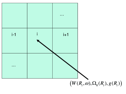
Figure 1: Illustration of our coarse graining approach to the local strong coupling solution of Eliashberg equations. We pixelize a finite system with the size of the patch to be on the order of $\xi$. Then we solve the selfconsistent strong pairing equations on each patch. The outcome of the solution is the set of local value for d-wave order parameter, that depends on the local value of boson frequency and local coupling constant. We present these values as a pixel dependent vector with these three components $(W({\bf R}_{i},\omega),\Omega_{0}({\bf R}_{i}),g({\bf R}_{i}))$.

With the recent STM experiments we now have an independent experimental measure of the local bosonic energy $\Omega_{0}({\bf R})$ as a function of position and doping Jinho1 . Typically, these energies are randomly distributed in a sample with characteristic variations on the length scale on the order of $20-50\AA$ and thus are consistent with our assumption of locality. The sample averaged frequency $\Omega_{0}=\langle\Omega_{0}({\bf R})\rangle$ is essentially doping independent and is about 52 meV, while distribution ranges between 40-70 meV for the observed bosonic modes in STM experiments, see Fig(1). We do not have a similar experimental information on coupling constant.

In practice, of course, only the total kernel $V$ will enter into the self-consistency equations and we would not be able to differentiate the effects of inhomogeneity in the $W$ due to electron-electron versus electron-lattice interaction inhomomgeneity. There is one important distinction however between electron-electron vs electron-lattice coupling. Electron-electron interaction being essentially frequency independent can not produce features outside the coherence peaks. Electron-lattice coupling on the other hand will produce the features in local tunneling characteristics at $\omega({\bf R})=\Delta({\bf R})+\Omega_{0}({\bf R})$. Hence the local tunneling characteristics would allow us to extract the inhomogeneous values of the bosonic modes, at least in principle. In practice one would have to deal with rather large signal- noise uncertainties but the local bosonic energy extraction from the dI/dV data can be done Jinho1 .

The local version of equations Eq(14,15) now would take a form:

$$W({\bf R},\omega_{n})=-T\sum_{m}V_{\omega_{n}-\omega_{m}}({\bf R})\langle F(\omega_{m},{\bf R},{\bf k}^{\prime})\rangle_{d}$$ (23)

and similarly for $S$:

$$S({\bf R},\omega_{n})=-T\sum_{m}V_{\omega_{n}-\omega_{m}}({\bf R})\langle G(\omega_{m},{\bf R},{\bf k}^{\prime})\rangle$$ (24)

and one can recognize standard Eliashberg equations that are now written locally, patch by patch. Hereafter we will approximate $S({\bf R},\omega_{n})=(1-Z_{\omega_{n}})i\omega_{n}$, i.e. local Z factor normalization only. In practice we know that effective mass renormalization in high-Tc materials is not very large and at most $Z\sim 2$, hence the effects of the normal self energy on quasipatrticle dispersion would be minor. It is the pairing interaction contribution from electron-boson interaction that we will be paying attention to. These equations in the homogeneous case were well analyzed. Eliashberg:60 ; McMillan:65 ; Scalapino:69

II.2 Weak Coupling Approximation

Now we will consider the weak coupling limit of these equations, namely the case when the pairing amplitude $W$ and normal self-energy corrections $S$ are small compared to the typical bosonic energy, $\Omega_{0}=\langle\Omega({\bf R})\rangle$. The most natural region to make the weak coupling approximation would be in the overdoped regime where both superconducting gap $\Delta$ and $T_{c}$ decrease with increased doping. There are no competing orders in the overdoped regime that would make the analysis more complicated. Competition with the other orders, like charge ordered state and pseudogap would make our analysis in terms of a single superconducting gap inaccurate. Therefore the analysis presented below assumes that we are dealing with optimally doped to overdoped samples.

Summation over Matsubara frequency in Eq.(23,24) is treated in a standard way by using $T\sum_{n}f(\omega_{n})=\oint dz\tanh(\frac{\beta z}{2})f(z),\beta=1/k_{B}T$. This integral is reduced to the integral over spectral density for the effective interaction that we will assume to be local:

$$V(\Omega) = \int_{-\infty}^{\infty}dx\frac{ImV(x)}{x-\Omega}$$

$$Im(g^{2}_{\Omega}({\bf R},{\bf R}^{\prime})B_{\Omega}({\bf R},{\bf R}^{\prime})) = g^{2}({\bf R})(\delta(\Omega-\Omega_{0}({\bf R}))-\delta(\Omega+\Omega_{0}({\bf R}))\delta_{{\bf R},{\bf R}^{\prime}}$$

$$ImV^{ee}({\bf R},{\bf R}^{\prime},\Omega) = V^{ee}({\bf R})\delta_{{\bf R},{\bf R}^{\prime}},\ \ |\Omega|\leq\Omega_{c}$$

$$ImV_{\Omega}({\bf R}) = ImV^{ee}({\bf R})-Img^{2}B_{\Omega}({\bf R})$$ (25)

where we have parametrized the position dependent electron-lattice interaction by local coupling constant $g^{2}$ and local boson frequency $\Omega_{0}({\bf R})$. Electron-electron interaction is assumed to be frequency independent up to cut-off frequency $\Omega_{c}\gg\Omega_{0}$.

Analysis we will implement here is essentially the same as the one used in standard Eliashberg approach. We use the d-wave projected propagator $F$ and integrate over the quasiparticle energies $\varepsilon({\bf k})$ to find from Eq(23,24):

$$W({\bf R},\Omega) = -N_{0}\int dx\int_{0}^{\infty}d\Omega^{\prime}\tanh(\frac{\beta\Omega}{2})\frac{Im(V_{x}({\bf R}))}{x-\Omega+\Omega^{\prime}}Re(\langle\frac{W({\bf R},\Omega^{\prime})}{\sqrt{(Z_{\Omega^{\prime}}\Omega^{\prime})^{2}-W^{2}({\bf R},{\bf k},\Omega^{\prime})}}\rangle_{{\bf k}})$$ (26)

$$= \int_{0}^{\infty}d\Omega^{\prime}N_{0}\frac{2g^{2}({\bf R})(\Omega_{0}({\bf R})+\Omega^{\prime})}{(\Omega_{0}({\bf R})+\Omega^{\prime})^{2}-(\Omega)^{2}+i\delta}Re(\langle\frac{W({\bf R},\Omega^{\prime})}{\sqrt{(Z_{\Omega^{\prime}}\Omega^{\prime})^{2}-W^{2}({\bf R},{\bf k},\Omega^{\prime})}}\rangle_{{\bf k}})$$

In the weak coupling limit for small coupling $g^{2}B(\omega,{\bf R})$ we can develop a local BCS pairing approximation for this local strongly coupled superconductor by approximating $W(\omega,{\bf R})=W(\omega=0,{\bf R})\Theta(\Omega_{0}({\bf R})-\omega),\omega>0$ and similar step like cut off at negative $\omega$.

We will focus on the low energy part of $W({\bf R},\Omega)$ that will contain real part of the gap only. Then a) the integral over $x$ is trivial since we assumed spectral function $ImV$ to be a delta function in frequency. We assume $T\rightarrow 0$ and hence $\tanh(\frac{\beta\Omega}{2})=1$. b) we assume that electron-electron part will produce normalizations on the normal channel and also will produce a d-wave pairing. Then we take a low frequency limit of this equation $\Omega\rightarrow 0$ and limit the integral over $\Omega^{\prime}$ over the range $\Omega^{\prime}\leq\Omega_{0}$ since the kernel is attractive only in this range. The weak coupling limit therefore would read as:

$$W({\bf R},\Omega=0) = \int_{0}^{\Omega_{0}({\bf R})}d\Omega^{\prime}N_{0}\frac{2g^{2}({\bf R})(\Omega_{0}({\bf R})+\Omega^{\prime})}{(\Omega_{0}({\bf R})+\Omega^{\prime})^{2}-(\Omega)^{2}+i\delta}$$

$$Re(\langle\frac{W({\bf R},\Omega=0)}{\sqrt{(Z_{\Omega^{\prime}}\Omega^{\prime})^{2}-W^{2}({\bf R},{\bf k},\Omega=0)}}\rangle_{{\bf k}})$$ (27)

and ultimately we obtain the local version of BCS equation for $W({\bf R})=W({\bf R},\Omega=0)$:

$$W({\bf R})=\int_{0}^{\Omega_{0}({\bf R})}d\Omega^{\prime}N_{0}g_{eff}({\bf R})Re(\langle\frac{W({\bf R})}{\sqrt{(Z_{\Omega^{\prime}}\Omega^{\prime})^{2}-W^{2}({\bf R},{\bf k},\Omega=0)}}\rangle_{{\bf k}})$$ (28)

with

$$g_{eff}({\bf R})=2\int d\omega\frac{g^{2}(\omega,{\bf R})B(\omega,{\bf R})}{\omega}$$ (29)

is a weak coupling limit coupling constant in Eliashberg theory.

Using the local approximation for the spectral density Eq.(25), we have

$$g_{eff}=2\frac{g^{2}({\bf R})}{\Omega_{0}({\bf R})}$$ (30)

Here we explicitly assume that $g({\bf R})$ and $\Omega({\bf R})$ are independent random distributions. This assumption is natural if we allow these two quantities to be set by local environment in the crystal and we do not assume here that coupling constant $g({\bf R})\sim(M\Omega({\bf R}))^{1/2}$ as would be the case for quantized extended collective modes. We thus arrive at the local gap equation for $\Delta({\bf R})=W({\bf R})/Z({\bf R})$:

$$\Delta({\bf R})=\Omega_{0}({\bf R})\exp(-\frac{1}{N_{0}g_{eff}({\bf R})})$$ (31)

Equation Eq.(31) is applicable in the weak coupling limit and therefore can be viewed only as a qualitative result. For any distribution of the coupling constants for small enough average value $<g^{2}B>$ there will be regions where this coupling constant is not smaller than $1$ and hence weak coupling analysis would fail in those regions. Nevertheless it is useful in that it allows us to analyze the results of numerical calculations, see below and compare numerical results with the locally observed quantities. With this caveat in mind we will consider the implications of the Eq.(31) for our analysis of the local pairing.

We find immediately three important consequences of the local pairing approximation: 1) Effective coupling constant is a function of the local boson mode energy. Effective coupling constant $g_{eff}({\bf R})$ is inversely proportional to the mode energy $\Omega_{0}({\bf R})$. This result implies that there is a direct negative correlation between local gap and local bosonic mode energy. Similar direct negative correlation is observed in the STM experiments on inelastic tunneling spectroscopy.Jinho1 2) Another implication of this result is that the isotope efffect will affect both the prefactor and coupling constant in Eq.(31). This point will be discussed more below. 3)Finally, from this simple equation we can find local effective coupling constant $N_{0}g_{eff}({\bf R})$ as:

$$N_{0}g_{eff}({\bf R})=-\frac{1}{\ln(\frac{\Delta({\bf R})}{\Omega_{0}({\bf R})})}$$ (32)

This equation contains two experimentally observable quantities: $\Delta({\bf R})$ and $\Omega_{0}({\bf R})$. We therefore can build the real space map of effective coupling constant.

III Numerical Results and Discussions

Here we will discuss the numerical solutions of local Eliashberg equation. From Eqs.(21) and (22) together with Eqs.(16) and (17), it can be written explicitly as:

$$i\omega_{n}S(\mathbf{R},i\omega_{n}) = -\frac{1}{N_{L}\beta}\sum_{\bf{q}}\sum_{i\Omega_{m}}\frac{M_{eff}(i\Omega_{m},{\bf R})}{\Pi(\mathbf{R},\mathbf{q};i\omega_{n}-i\Omega_{m})}[(i\omega_{n}-i\Omega_{m})Z(\mathbf{R},\mathbf{q};i\omega_{n}-i\Omega_{m})+\xi_{\mathbf{q}}\;,$$

$$W({\bf R},i\omega_{n}) = -\frac{2}{N_{L}\beta}\sum_{\mathbf{q}}\sum_{i\Omega_{m}}\frac{M_{eff}(i\Omega_{m},\mathbf{R})}{\Pi(\mathbf{R},\mathbf{q};i\omega_{n}-i\Omega_{m})}W(\mathbf{R},\mathbf{q};i\omega_{n}-i\Omega_{m})\;,$$ (33a)

where

$$M_{eff}(\mathbf{R},\mathbf{k};i\Omega_{m})=[V_{ee}(\mathbf{R})-g^{2}(\mathbf{R})B(\mathbf{R},i\Omega_{m})]\eta_{\mathbf{k}}\;$$ (34)

with

$$B(\mathbf{R};i\Omega_{m})=\frac{1}{i\Omega_{m}-\Omega_{0}(\mathbf{R})}-\frac{1}{i\Omega_{m}+\Omega_{0}(\mathbf{R})}\;,$$ (35)

and

$$\Pi(\mathbf{R},\mathbf{k};i\omega_{n})=\{[i\omega_{n}Z(\mathbf{R},\mathbf{q};i\omega_{n})^{2}-[\xi_{{\bf k}}^{2}+W^{2}(\mathbf{R},\mathbf{k};i\omega_{n})]^{2}\}^{1/2}\;.$$ (36)

Note that the strong correlation between electrons themselves can give rise to an effective pairing. In this case, $v_{ee}$ is negative. In principle, we cannot exclude the possibility that $v_{ee}$ also becomes inhomogeneous. Here we focus on the effect from the electron coupled to local modes and will ignore the contribution from $v_{ee}$. We mention equation for normal self-energy correction for completeness. As was pointed out, we will ignore $S$.

We adopt a six-parameter fit to the band structure used previously for optimally doped Bi-2212 systems, Norman:95 having the form

$$\xi_{\mathbf{k}} = -2t_{1}(\cos k_{x}+\cos k_{y})-4t_{2}\cos k_{x}\cos k_{y}$$ (37)

$$-2t_{3}(\cos 2k_{x}+\cos 2k_{y})$$

$$-4t_{4}(\cos 2k_{x}\cos k_{y}+\cos k_{x}\cos 2k_{y})$$

$$-4t_{5}\cos 2k_{x}\cos 2k_{y}-\mu\;,$$

where $t_{1}=1$, $t_{2}=-0.2749$, $t_{3}=0.0872$, $t_{4}=0.0938$, $t_{5}=-0.0857$, and $\mu=-0.8772$. Unless specified explicitly, the energy is measured in units of $t_{1}$ hereafter.

We use the method of Vidberg and Serene to first solve the above coupled equations in the Matsubrara frequency space. On Matsubara axis the quantities $S$ and $W$ are real. We then do the analytical continuation with the Pade approximation to covert them to the axis of real frequency, on which they have a real and imaginary part. Partly motivated by the ARPES experiments Bogdanov00 ; Kaminski01 ; Lanzara01 ; Johnson01 ; Zhou03 ; Kim03 ; Gromko03 ; Sato03 ; Cuk04 ; Zhou05 , we take the averaged frequency of the local bosonic modes to be $\langle\Omega_{0}\rangle=0.3$ and the bare electron-bosonic mode coupling constant $\langle g_{0}\rangle=0.5$. The temperature is chosen at $T=0.01$. To be illustrative, we first show the calculation at a specific coarse-grained spatial point. Our calculations show that $S$ is negligible and we will ingore it hereafter.

III.1 Relation between features of the gap and coupling constant and bosonic energy

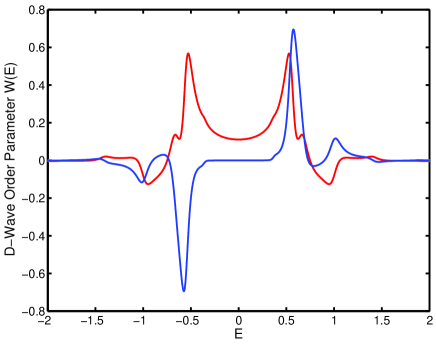
Figure 2: The real (red line) and imaginary (blue line) parts of the complex $d$-wave order parameter as a function of energy. Here the bosonic mode frequency $\Omega_{0}=0.3$ and the electron-mode coupling constant $g_{0}=0.5$.

In Fig.(2) we can see that at low energies the real part is constant and imaginary part rises only after energy exceeds the boson energy $\Omega_{0}=0.3$. The first peak of $ReW$ curve and shoulder on $ImW$ curve precisely correspond to the boson energy. Features at higher energies correspond to the multiboson processes and are at multiples of $\Omega_{0}$. In Fig.(3) we observe the evolution of the inelastic features as a function of coupling constant. Gap function is changing substantially even for fixed boson energy. Still there is always a feature at boson energy for all coupling constants. For larger energies and larger coupling constants peaks in $ReW$ are getting broader. In Fig.(4) the features in the the real part of gap function for different values of boson energy are shown. Again the first shoulder albeit of different intensity can be seen at energy that exactly corresponds to the boson energy. Feature at $E=0.2$ for blue curve is very broad, the one at $E=0.3,0.6$ can be seen for boson energy $\Omega_{0}=0.3$ and finally for the green curve one can see feature at $E=0.4$. Features at substantially higher energies are likely to be numerical artifacts of our use of Pade approximations in analytic continuation.

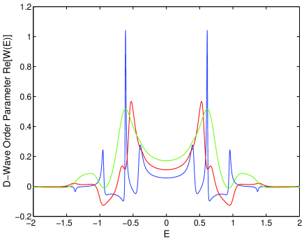
Figure 3: The real part of the complex $d$-wave order parameter as a function of energy for various values of the electron-mode coupling constant $g_{0}=0.4$ (blue line), $0.5$ (red line), $0.6$ (green line). The bosonic mode frequency is fixed at $\Omega_{0}=0.3$.

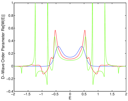
Figure 4: The real part of the complex $d$-wave order parameter as a function of energy for various values of the mode frequency $\Omega_{0}=0.2$ (blue line), $0.3$ (red line), $0.4$ (green line). The bare electron-mode coupling constant is fixed at $g_{0}=0.5$.

III.2 Correlation between inhomogeneous coupling constant and gap; anticorrelation between bosonic mode energy and gap

Next we consider the effect of electronic inhomogeneity. For this purpose, we consider two cases, a) coupling constant has a spatial distribution and b) local bosonic mode has a spatial distribution. Both of these parameters can be position dependent at the same time as we suspect is the case in real systems. Here we want to differentiate between the effects coming from coupling constant and effects coming from frequency variations. We assume that both distributions are gaussians.

$$P(x)\propto\exp\biggl{[}\frac{(x-\langle x\rangle)^{2}}{2\alpha^{2}}\biggl{]}\;,$$ (38)

where $x$ represents $g_{0}$ or $\Omega_{0}$. Throughout the work, we take $\alpha=0.3$.

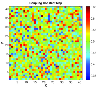
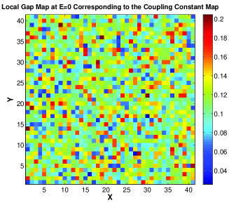
Figure 5: The spatial distributions of the bare coupling constant (left panel) and the resultant $d$-wave order parameter at zero energy. The bosonic mode frequency is fixed at $\Omega_{0}=0.3$.

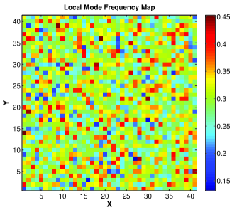
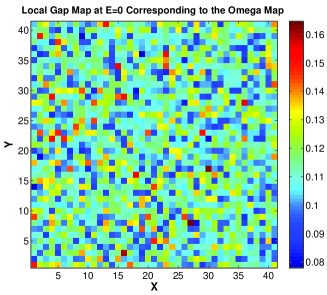
Figure 6: The spatial distributions of the mode frequency (left panel) and the resultant $d$-wave order parameter at zero energy. The bare electron-mode coupling constant is fixed at $g_{0}=0.5$. Anticorrelation between the mode frequency and gap magnitude is clearly seen. Large mode frequency regions (red spots in the left panel) correlate with the small gap regions (dark spots in the right panel). Anticorrelation for arbitrary coupling constant is thus verified numerically. In the weak coupling limit the anticorrelation follows from Eq. (29,30).

In Fig(5) we observe the direct correlation between the strength of the coupling constant and $ReW(E=0)$. This direct correlation is natural and to be expected. In Fig. (6) we find an anticorrelation between the boson mode energy and gap energy. The nature of this anticorrelation follows from our assumption on the boson spectral function that is peaked at one energy $\Omega_{0}$. Indeed from the structure of the pairing kernel one can see that larger boson energy at fixed $g$ would lead to lower effective coupling constant, see Eq.(29). Thus we conclude that the anticorrelation is not a consequence of the weak coupling analysis but is present in the full numerical solution of the self-consistent gap equations. This anticorrelation is directly observed in the IETS STM experiments.Jinho1

III.3 LDOS map and the $d$-wave order parameter map

We have also calculated the local density of states (LDOS).

$$\rho(E)=\frac{2}{N_{L}\pi}\sum_{\mathbf{k}}|\text{Im}\mathcal{G}(\mathbf{R},\mathbf{k};E+i0^{+})|\;,$$ (39)

which correspond to the local differential tunneling conductance as measured by the STM experiments. Fig.(7) shows the local density of states as a function of energy at a selected spatial point corresponding to Fig.1. For comparison we also show typical experimental data for STM tunneling density of states and its derivative, Fig(7)

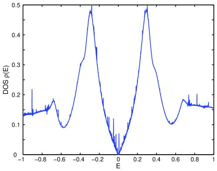
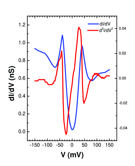
Figure 7: The density of states as a function of energy. Here the bosonic mode frequency $\Omega_{B}=0.3$ and the electron-mode coupling constant $g_{0}=0.5$. Also shown is an experimentally measured $dI/dV$ and $d^{2}I/dV^{2}$ spectra at some typical point are shown. The overall similarity of the spectrum with the one we have calculated is suggestive that the features in the tunneling seen at the large bias are indeed consistent with the strong coupling features due to electron-boson interactions.

We also calculated spatial image of the LDOS at the energy $\Delta_{g}$. In the strong-coupling theory, the $d$-wave order parameter is energy dependent. To demonstrate the distribution of gap inhomogeneity from the LDOS distribution at the gap edge $\Delta_{g}$, we should use the $d$-wave order parameter at fixed energy, say $E=<\Delta>$. Fig(8) shows spatial distribution of the LDOS for the case of an inhomogeneous distribution of local bosonic modes.

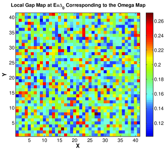
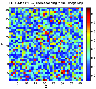
Figure 8: The spatial distributions of the real part of the $d$-wave order parameter at $E=\Delta_{g}$ (left panel) and the local density of states at the same energy. The bare electron-mode coupling constant is fixed at $g_{0}=0.5$.

IV Isotope Effect in Inhomogeneous Superconductor

One of the most powerful tools to investigate the role of phonons in the pairing is to study isotope effect. In the case of conventional supercoductors it was found that isotope subsitution of the lattice atoms would change the transiton temperature thus directly indicating that lattice is involved in pairing. By changing the mass of the ions from M to M’ critical temperature $T_{c}\sim M^{-\alpha}$ would change by $T_{c}^{\prime}/T_{c}=(M/M^{\prime})^{\alpha}$.

First consider conventional homogeneous superconductors. In conventional superconductors often $\alpha\simeq 1/2$ is observed. This result follows the observation that the effective coupling constant in standard BCS formalism is independent of mass M.Scalapino:69 Simple arguments show that effective coupling constant in homogeneous case $g_{eff}=\frac{C}{M\omega^{2}_{av}}$, where $C$ is a constant, $M$ is the ion mass and $\omega^{2}_{av}$ is the average phonon frequency squared. Since $\omega_{av}\sim M^{-1/2}$ for phonon spectrum regardless of the detailed shape, one finds that the coupling constant in this case is independent of mass $M$. Therefore the only effect of the isotope substitution is on the change of the phonon spectrum and the cutoff frequency that is in the prefactor in BCS equation for

$$T_{c}=\Omega_{0}\exp(-\frac{1}{N_{0}g_{eff}})$$ (40)

We thus find the conventional exponent is $\alpha=1/2$ that is set solely by the prefactor $\Omega_{0}$ within the BCS theory. Situation we consider is very different. As we pointed out, $g_{eff}({\bf R})$ is made from two random independent quantities, $g({\bf R})$ and $\Omega_{0}({\bf R})$. This will lead to a very different isotope effect in this random superconductor.

Standard isotope substitution experiment in cuprates is replacement of ${}^{16}O$ by ${}^{18}O$. The changes in $T_{c}$ produced by this substitution are small, $\alpha$ is small and depend on doping levels of the samples. In the optimally doped samples $\alpha$ is essentially zero.

Situation for inhomogeneous superconductors is qualitatively different from conventional BCS case. Inhomogeneous superconductor is characterized by two rather than one parameter that enters into the gap equation Eq.(22): one is coupling constant $g({\bf R})$ and another one is a local boson frequency $\Omega_{0}({\bf R})$. In principle, both random variable will change upon isotope substitution. On general grounds, isotopic substitution would change the local environement as it affects both in-plane and out of-plane oxygen atoms. Hence, we argue that both the coupling constant and phonon frequency are affected by isotope substitution. It would mean therefore that both prefactor and coupling constant in the exponent are changed in Eq.(31) upon ${}^{16}O$ to ${}^{18}O$ substitution. In addition, for the inhomogeneous superconductor one has to differentiate between the isotope shift of critical temperature of a sample $T_{c}$ and the isotope shift of the gap $\Delta({\bf R})$. Here we do not address the net shift of $T_{c}$ as it is determined by phase fluctuations at higher temperatures. Instead we focus on shift of local gap $\Delta({\bf R})$ or average gap $<\Delta({\bf R})>$.

$$\Delta({\bf R})=\Omega_{0}({\bf R})\exp(-\frac{1}{N_{0}g_{eff}({\bf R})})$$ (41)

Again for simplicity we will take a weak coupling limit of inhomogeneous Eliashberg equations. Let us take an ”average” of the equation as an approximate way to discuss the average shifts in $\Omega_{0}({\bf R})$ and in $N_{0}g_{eff}({\bf R})$, Eq.(41)

$$\langle\Delta({\bf R})\rangle=\langle\Omega_{0}({\bf R})\rangle\exp(-\frac{1}{\langle N_{0}g_{eff}({\bf R})\rangle})$$ (42)

It is known Jinho1 that the average frequency $\Omega_{0}=\langle\Omega_{0}({\bf R})\rangle$ shifts from 52 meV to 48 meV upon ${}^{16}O$ by ${}^{18}O$ substitution. On the other hand this shift in $\Omega_{0}$ can be offset by a shift in average $g_{eff}$ thus producing an zero isotope effect that is very different from BCS exponent $\alpha_{BCS}=1/2$. To illustrate how one gets near zero isotope shift, we take that effective coupling constant shifts by

$$\ln(\frac{\Omega_{0}}{\Omega^{\prime}_{0}})=\frac{1}{N_{0}g_{eff}}-\frac{1}{N_{0}g^{\prime}_{eff}}$$ (43)

This shift of the effective coupling constant could offset the shift of the prefactor in Eq.(42). The net isotope effect will be determined by the combined isotope shift of the boson mode energy and effective coupling constant. They can mutually cancel each other making net effect small, as we suspect is the case near optimal doping. Alternatively, both effects can add up to produce large isotope shift. Thus by knowing only the shift of boson energy is not sufficient to address the net isotope effect of the gap.

To illustrate this point we have preformed ”numerical isotope shift” experiment within our model, see Fig(9). In order to model the effect of oxygen subtitution we change random distribution $P(\Omega_{0})$ of the boson energy $\Omega_{0}$. We assumed that changing ${}^{16}O$ to ${}^{18}O$ would shift gaussian distribution with the mean values of boson energy $\langle\Omega_{0}\rangle_{O16}=\overline{\Omega}=0.3$ to $\langle\Omega_{0}\rangle_{O18}=\overline{\Omega}(1-6\%)$ ( upper panel). At the same time coupling constant $g$ can also change upon isotope substitution. We consider the shift in the coupling constant $g$ which here is taken to be constant at the same time (lower panel). For ${}^{16}O$ we take $g=g_{0}=0.5$ and for ${}^{18}O$ we use $g_{0}(1-4\%)$. We find that negative shift of boson energy by $6\%$ can be offset by the shift of the coupling constat $g_{0}$ and the net effect would be negative shift of the gap $\langle W\rangle$. To address the net isotope effect it is necessary to measure independently both boson energy and coupling constat for ${}^{16}O$ and ${}^{18}O$. At moment there is no independent experimental measurement of the coupling constant we are aware of.

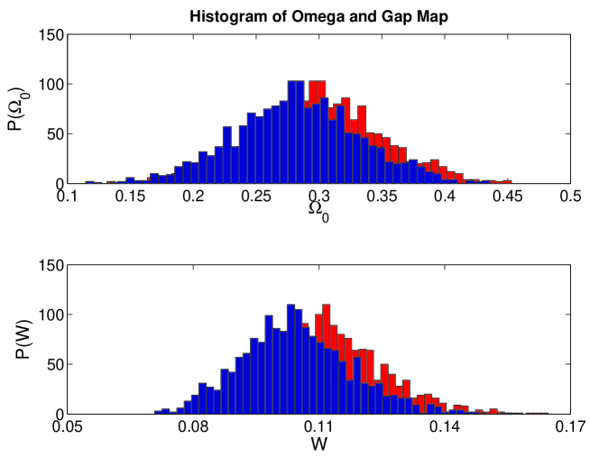
Figure 9: Upper panel: histograms of (the boson energy $\Omega_{0}$ (upper panel) for $O^{16}$ (red) and $O^{18}$ (blue) are shown assuming $6\%$ isotope shift. Lower panel: histograms of the calculated gap distribution $W$ for these two boson mode distribution calculated with simultaneous coupling constant shift. We assumed that coupling relative constant shift is negative $4\%$. This turns to be sufficient to produce net negative gap shift.

For completeness we also present the correlation between the gap and the mode energy $\Omega_{0}$, Fig(10). The negative correlation between the gap and mode energy is clearly seen for both $O^{16}$ and $O^{18}$ isotopes.

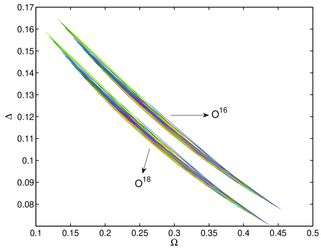
Figure 10: From the real space maps for mode energy $\Omega_{0}$ and gap as a function of position we can extract the statistical cross-correlation of these two quantities. We find overall negative concave-shaped $\Delta$-$\Omega_{0}$ cross correlation for the cases of $O^{16}$ and $O^{18}$. Isotope shift of mode energy to lower energies is clearly seen on this plot. The average gap value is affected by the shift in the coupling constant and in mode energy.

V Conclusion

In this paper we use strong coupling model for boson mediated d-wave pairing for inhomogeneous superconductor. To model inhomogeneous superconductor we consider a coarse grain model with the typical size of the patch on the order of superconducting coherence length $\xi\sim 20-50\AA$. We use patch dependent pairing interaction due to disordered pairing boson with patch-dependent coupling constant $g({\bf R})$ and boson energy $\Omega_{0}({\bf R})$. This local pairing produces local superconducting gap as a selfconsistent solution of Eliashberg equations patch by patch.

We argue that any inhomogeneous theory of strong coupling theory of pairing has to involve at least two independent quantities that characterize electron-boson interaction: coupling constant and boson energy. Reduction of the pairing theory to an inhomogeneous BCS pairing model does not allow one to distinguish a relative role of the coupling constant $g({\bf R})$ vs $\Omega_{0}({\bf R})$. In BCS-like analysis one deals with the single effective coupling $g_{eff}({\bf R})$ that is combination of $g({\bf R})$ and $\Omega_{0}({\bf R})$, Eq.(30).

We use the local coupling constant and boson energy drawn randomly with the gaussian distributions and calculate local gap function $W(\omega,{\bf R})=ReW(\omega,{\bf R})+iImW(\omega,{\bf R})$. This gap map is then used to compare correlations between $W({\bf R})$, $g({\bf R})$ and $\Omega_{0}({\bf R})$. We also calculate the local tunneling density of states that is consistent with the observed by STM density of states.

Numerically we find a direct positive correlation between the gap map $W({\bf R})$ and boson coupling constant map. This is not surprising: the larger the coupling the larger is gap function. We also find an interesting and surprising result that there is a negative correlation between gap function scale and boson mode energy $\Omega_{0}$. We give a simple interpretation of this negative correlation in the case of the weak coupling analysis. We find that effective BCS coupling constant is inversely proportional to the boson energy, Eq.(30). Because effective coupling constant is in the exponent of a gap solution Eq.(31), its dependence on $\Omega_{0}({\bf R})$ is more important than the dependence on frequency in the prefactor. Larger frequency boson is less effective in inducing pairing for fixed $g({\bf R})$ in our model. This result is consistent with the experimental observation of the IETS signal, where anticorrelation between gap and boson mode energy was observed. Jinho1

Exact nature of the boson is not important for our analysis except when we discuss isotope effect. Then we expicitly assume that boson is a lattice mode and its energy has on average an isotope shift consistent with the isotope shift for phonons due to ${}^{16}O$ to ${}^{18}O$ substitution.

We also consider isotope effect. We find that in order to correctly address the full isotope effect one again would need to have assess changes in the coupling constant $g({\bf R})$ and $\Omega_{0}({\bf R})$ as a result of ${}^{16}O$ to ${}^{18}O$ isotope substitution. Both shift in the boson frequency and coupling constant contribute to the net isotope effect and we find that small, on the order of $\sim 4\%$, changes of the coupling constant can completely offset the isotope shift of the gap function $W({\bf R})$ caused by the standard isotope effect for the lattice mode $\Omega_{0}({\bf R})$.

We therefore find that in order to understand the isotope effect in d-wave superconductors we would need independent measurements of the coupling constant map and boson mode energy map for different isotopes. The whole notion that a single isotope exponent can characterise the spatially modulated superconducting state as is the case of high-Tc materials seem to be too simplistic to address the real situation. It appears one can not make an evaluation on the importance of the lattice effects in high-Tc superconductors based on a shift of a critical temperature without addressing the changes of the gap, boson modes and coupling constant.

To address the effects of spatial inhomogeneity of tunneling IETS spectra we focus on electron-boson coupling, ignoring electron-electron interaction part that will not produce IETS features. Electron-boson interaction is only one contribution to the pairing interactions. Pairing in high-$T_{c}$ materials is likely a result of interplay between strong electron-electron correlations and electron-boson interaction. The realistic magnitude of pairing interaction and how large the transition temperature would be by assuming only electron-boson pairing is an interesting question. We leave this question for a separate investigation.

- (1) G. M. Eliashberg, Sov. Phys. JETP 11, 696 (1960).
- (2) W. L. McMillan and J. M. Rowell, Phys. Rev. Lett. 14, 108 (1965); W. L. McMillan and J. M. Rowell, in Superconductivity, Vol. 1, edited by R. D. Parks (Dekker, New York, 1969).
- (3) D. J. Scalapino, in Superconductivity, Vol. 1, edited by R. D. Parks (Dekker, New York, 1969).
- (4) J. P. Carbotte, Rev. Mod. Phys. 62, 1027 (1990).
- (5) I. Giaever, Phys. Rev. Lett. 5, 464 (1960); J. C. Fisher and I. Giaever, J. Appl. Phys. 32, 172 (1961); I. Giaever, Phys. Rev. Lett. 5, 146 (1966).
- (6) Q. Huang, J. F. Zasadzinski, K. E. Gray, J. Z. Liu, and H. Claus, Phys. Rev. B 40, 9366 (1989).
- (7) Ch. Renner and Ø. Fischer, Phys. Rev. B 51, 9208 (1995).
- (8) Ch. Renner, B. Revaz, J.-Y. Genoud, and Ø. Fischer, J. Low Temp. Phys. 105, 1083 (1996).
- (9) Y. DeWilde, N. Miyakawa, P. Guptasarma, M. Iavarone, L. Ozyuzer, J. F. Zasadzinski, P. Romano, D. G. Hinks, C. Kendziora, G. W. Crabtree, and K. E. Gray, Phys. Rev. Lett. 80, 153 (1998).
- (10) D. Mandrus, L. Forro, D. Koller, and L. Mihaly, Nature 351, 460 (1991).
- (11) A. Yurgens, D. Winkler, T. Claeson, S.-J. Hwang, and J.-H. Choy, Int. J. Mod. Phys. B 29-31, 3758 (1999).
- (12) J.F. Zasadzinski, L. Ozyuzer, N. Miyakawa, D. G. Hinks, K. E. Gray, Physica C 341-348, 867 (2000).
- (13) J. F. Zasadzinski, L. Ozyuzer, N. Miyakawa, K. E. Gray, D. G. Hinks, and C. Kendziora, Phys. Rev. Lett. 87, 067005 (2001).
- (14) D. S. Dessau, B. O. Wells, Z. X. Shen, W. E. Spicer, A. J. Arko, R. S. List, D. B. Mitzi, A. Kapitulnik, Phys. Rev. Lett. 66, 2160 (1991).
- (15) H. Ding, A. F. Bellman, J. C. Campuzano, M. Randeria, M. R. Norman, T. Yokoya, T. Takahashi, H. Katayama-Yoshida, T. Mochiku, K. Kadowaki, G. Jennings, and G. P. Brivio, Phys. Rev. Lett. 76, 1533 (1996).
- (16) Z.X. Shen et al., Phys. Rev. Lett., 70, 1553 (1993).
- (17) J. C. Campuzano, H. Ding, M. R. Norman, H. M. Fretwell, M. Randeria, A. Kaminski, J. Mesot, T. Takeuchi, T. Sato, T. Yokoya, T. Takahashi, T. Mochiku, K. Kadowaki, P. Guptasarma, D. G. Hinks, Z. Konstantinovic, Z. Z. Li, and H. Raffy Phys. Rev. Lett. 83, 3709 (1999).
- (18) P. V. Bogdanov, A. Lanzara, S. A. Kellar, X. J. Zhou, E. D. Lu, W. J. Zheng, G. Gu, J.-I. Shimoyama, K. Kishio, H. Ikeda, R. Yoshizaki, Z. Hussain, and Z. X. Shen, Phys. Rev. Lett. 85, 2581 (2000).
- (19) A. Kaminski, M. Randeria, J. C. Campuzano, M. R. Norman, H. Fretwell, J. Mesot, T. Sato, T. Takahashi, and K. Kadowaki, Phys. Rev. Lett. 86, 1070 (2001).
- (20) A. Lanzara, P. V. Bogdanov, X. J. Zhou, S. A. Kellar, D. L. Feng, E. D. Lu, T. Yoshida, H. Eisaki, A. Fujimori, K. Kishio, J.-I. Shimoyama, T. Noda, S. Uchida, Z. Hussain, Z.-X. Shen, Nature 412, 510 (2001); Gweon, G.-H. et al. Nature 430, 187 190 (2004).
- (21) P. D. Johnson, T. Valla, A. V. Fedorov, Z. Yusof, B. O. Wells, Q. Li, A. R. Moodenbaugh, G. D. Gu, N. Koshizuka, C. Kendziora, Sha Jian, and D. G. Hinks, Phys. Rev. Lett. 87, 177007 (2001).
- (22) X. J. Zhou, T. Yoshida, A. Lanzara, P. V. Bogdanov, S. A. Kellar, K. M. Shen, W. L. Yang, F. Ronning, T. Sasagawa, T. Kakeshita, T. Noda, H. Eisaki, S. Uchida, C. T. Lin, F. Zhou, J. W. Xiong, W. X. Ti, Z. X. Zhao, A. Fujimori, Z. Hussain, Z.-X. Shen, Nature 423, 398 (2003).
- (23) T. K. Kim, A. A. Kordyuk, S. V. Borisenko, A. Koitzsch, M. Knupfer, H. Berger, and J. Fink, Phys. Rev. Lett. 91, 167002 (2003).
- (24) A. D. Gromko, A. V. Fedorov, Y.-D. Chuang, J. D. Koralek, Y. Aiura, Y. Yamaguchi, K. Oka, Yoichi Ando, and D. S. Dessau, Phys. Rev. B 68, 174520 (2003).
- (25) T. Sato, H. Matsui, T. Takahashi, H. Ding, H.-B. Yang, S.-C. Wang, T. Fujii, T. Watanabe, A. Matsuda, T. Terashima, and K. Kadowaki, Phys. Rev. Lett. 91, 157003 (2003).
- (26) T. Cuk, F. Baumberger, D. H. Lu, N. Ingle, X. J. Zhou, H. Eisaki, N. Kaneko, Z. Hussain, T. P. Devereaux, N. Nagaosa, and Z.-X. Shen, Phys. Rev. Lett. 93, 117003 (2004).
- (27) X.J. Zhou et al., Phys. Rev. Lett. 95, 117001 (2005).
- (28) T. Dahm, D. Manske, D. Fay, and L. Tewordt, Phys. Rev. B 54, 12006 (1996); T. Dahm, D. Manske, and L. Tewordt, Phys. Rev. B 58, 12454 (1998).
- (29) Z. X. Shen and J. R. Schrieffer, Phys. Rev. Lett. 78, 1771 (1997).
- (30) M. R. Norman, H. Ding, J. C. Campuzano, T. Takeuchi, M. Randeria, T. Yokoya, T. Takahashi, T. Mochiku, and K. Kadowaki, Phys. Rev. Lett. 79, 3506 (1997).
- (31) M. R. Norman and H. Ding, Phys. Rev. B 57, R11089 (1998).
- (32) Ar. Abanov and A. V. Chubukov, Phys. Rev. Lett. 83, 1652 (1999); Phys. Rev. B 61, R9241 (2000).
- (33) M. Eschrig and M. R. Norman, Phys. Rev. Lett. 85, 3261 (2000); Phys. Rev. B 67, 144503 (2003).
- (34) M. R. Norman, M. Eschrig, A. Kaminski, and J. C. Campuzano, Phys. Rev. B 64, 184508 (2001).
- (35) D. Manske, I. Eremin, and K. H. Bennemann, Phys. Rev. lett. 87, 177005 (2001).
- (36) Ar. Abanov, A. V. Chubukov, and J. Schmalian, Adv. Phys. 52, 119 (2003).
- (37) A. W. Sandvik, D. J. Scalapino, and N. E. Bickers, Phys. Rev. B 69, 094523 (2004).
- (38) T. P. Devereaux, T. Cuk, Z.-X. Shen, and N. Nagaosa, Phys. Rev. Lett. 93, 117004 (2004).
- (39) T. Cren et al., Phys. Rev. Lett. 84, 147 (2000); Europhys. Lett. 54, 84 (2001).
- (40) C. Howald, P. Fournier, and A. Kaptitulnik, Phys. Rev. B 64, 100504 (2001).
- (41) S. H. Pan et al., Nature 413, 282 (2001).
- (42) K. M. Lang et al., Nature 415, 412 (2002).
- (43) A. C. Fang et al., Phys. Rev. B 70, 214514 (2004).
- (44) K. McElroy et al., Science 309, 1048 (2005).
- (45) J. H. Lee et al., unpublished. J. Lee, K. McElroy, J. Slezak, S. Uchida, H. Eisaki, and J.C. Davis, Bull. Am. Phys. Soc. 50(2005) 299. J.C. Davis, J. Lee, K. McElroy, J. Slezak, H. Eisaki, and S. Uchida, Bull. Am. Phys. Soc. 50(2005)1223.
- (46) T. S. Nunner, B. M. Anderson, A. Melikyan, and P. J. Hirschfeld, Phys. Rev. Lett. 95, 177003 (2005).
- (47) M.R. Norman, M. Randeria, H. Ding and J.C. Campuzano, Phys. Rev. B 52, 615, (1995).