Two-Dimensional Scaling Limits
via Marked Nonsimple Loops

Abstract

We postulate the existence of a natural Poissonian marking of the double (touching) points of $SLE_{6}$ and hence of the related continuum nonsimple loop process that describes macroscopic cluster boundaries in 2D critical percolation. We explain how these marked loops should yield continuum versions of near-critical percolation, dynamical percolation, minimal spanning trees and related plane filling curves, and invasion percolation. We show that this yields for some of the continuum objects a conformal covariance property that generalizes the conformal invariance of critical systems. It is an open problem to rigorously construct the continuum objects and to prove that they are indeed the scaling limits of the corresponding lattice objects.

Keywords: scaling limits, percolation, near-critical, minimal spanning tree, finite size scaling, conformal covariance.

1 Introduction

The rigorous geometric analysis of the continuum scaling limit of two-dimensional critical percolation has made much progress in recent years. This work has focused on triangular lattice site percolation, or equivalently random (white-black) colorings of the faces of the hexagonal lattice, where the critical value of the probability $p$ for a hexagon to be white is $p_{c}=1/2$. A key breakthrough was the realization [20] (proved in [23, 11]) that when the lattice spacing $\delta\to 0$, the limit of the $p=p_{c}$ lattice exploration path must be chordal $SLE_{6}$. This result was extended in [8, 10] to obtain the “full scaling limit” at $p=p_{c}$ of all macroscopic cluster boundaries as a certain $SLE_{6}$-based process of continuum nonsimple loops in the plane.

In this paper, we propose an approach for obtaining the one-parameter family of near-critical scaling limits where $p=p_{c}+\lambda\delta^{\theta}$ as $\delta\to 0$ with $\lambda\in(-\infty,\infty)$ and $\theta$ chosen ($=3/4$ as in, e.g., [6]) to get nontrivial $\lambda$-dependence in the limit (see also the discussions in [1, 2]). We do not present any theorems here but rather use heuristic arguments to provide what we believe is the correct (or, at least, a correct) conceptual framework for not only scaling limits of near-critical percolation but also, as we shall explain later, for related 2D scaling limits such as of continuum percolation, Dynamical Percolation (DP), the Minimal Spanning Tree (MST) and Invasion Percolation (IP). Our purpose is to encourage work on the various problems associated with what we hope will be the eventual rigorous implementation of this framework.

The framework relies on a postulated (natural) Poissonian “marking” of the double points (touching points) of $SLE_{6}$ and hence of the continuum nonsimple loops of the full scaling limit at $p=p_{c}$. Part of the motivation for such an approach is that an analogous one succeeded in the simpler “Brownian Web” setting. There, in place of $SLE_{6}$ double points, there were points in $(1+1)$-dimensional space-time from which two distinct paths emerge [14]. In the Brownian Web setting, the Poissonian marking turned out to be rather straightforward to implement. An essential open problem, as discussed in Section 2 after we review some properties of $SLE_{6}$ and the critical loop process, is to find a rigorous implementation of the postulated marking in the $SLE_{6}$ setting. Key steps are to construct the correct intensity measure supported on $SLE_{6}$ double points and show that it is the limit of the appropriate scaled counting measure on the lattice.

In Sections 3-8, we then use the marked critical loops to construct continuum versions of various lattice objects: near-critical white clusters (Section 3), near-critical loops (Section 4), (critical) dynamical percolation (Section 5), near-critical exploration paths (Section 6), minimal spanning trees and related lattice-filling curves (Section 7), and invasion percolation (Section 8).

2 Marking the critical loops

In the critical ($p=1/2$) or near-critical ($p=1/2+\lambda\delta^{\theta}$) random coloring of the faces of the hexagonal lattice (with lattice spacing $\delta$), we focus on the macroscopic white and black clusters, whose diameters are $\geq\varepsilon>0$ as $\delta\to 0$ (where $\varepsilon$ is arbitrary and will also be taken to $0$ eventually). We consider the outer boundaries of these clusters as a collection $X_{\epsilon}^{\delta}$ of simple closed curves in the plane (modulo reparametrization – see [3, 9, 10] for technical details about this and other issues) – see Figure 1 – which we regard as oriented with a counterclockwise (respectively, clockwise) orientation for the white (resp., black) clusters. The limit in distribution, as $\varepsilon,\delta\to 0$, of this family of macroscopic cluster boundaries at $p=1/2$ is what we call the (critical) continuum nonsimple loop process or simply critical loop process $X$ (with distribution $P$). Here are a few of the almost sure properties of $X$ (or $P$).

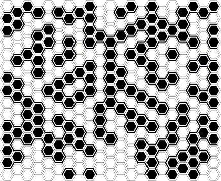
Figure 1: Finite portion of a (site) percolation configuration on the triangular lattice with each hexagon representing a site assigned one of two colors. In the critical percolation model, colors are assigned randomly with equal probability. The cluster boundaries are indicated by heavy lines; some small loops appear, while other boundaries extend beyond the finite region depicted.

• There are countably many loops, all continuous.

• Loops do not cross themselves or each other.

• Loops are nonsimple – touching themselves and each other.

• All touching points are double points – there are no points in the plane touched in total $3$ or more times (by $1,2$ or $3$ loops).

• For any deterministic point $z$ and $0<r_{1}<r_{2}<\infty$, the number ${\cal N}(z,r_{1},r_{2})$ of loops surrounding $z$ that are contained in the annulus centered at $z$ with inner (resp., outer) radius $r_{1}$ (resp., $r_{2}$) is finite but tends to infinity as $r_{1}\to 0$ or $r_{2}\to\infty$.

• For any two loops $L,L^{\prime}$, there is a finite sequence of loops $L_{1}=L$, $L_{2}$, $\ldots,L_{M}=L^{\prime}$ such that $L_{i}$ touches $L_{i+1}$ for each $i=1,\ldots,M-1$.

• Every loop $L$ has a unique “parent” loop $L^{*}$ which surrounds $L$ (with no intermediate loop surrounding $L$); $L^{*}$ has opposite orientation to $L$; $L$ has infinitely many “daughter” loops.

We also note that the distribution of the critical loop process has various conformal invariance properties including invariance under translations, rotations and scalings of the plane.

The critical loop process may be constructed in the continuum by a procedure in which each loop is a concatenation of two paths, each of which is distributed as (all or part of) a chordal $SLE_{6}$ process – the Schramm-Loewner evolution with parameter $6$. This is of course based on the result [20, 23, 11] that chordal $SLE_{6}$ is the scaling limit as $\delta\to 0$ of the critical percolation exploration path in the closure $\overline{D}$ of a domain $D$, from $a$ to $b$ on the boundary $\partial D$. The exploration path may be thought of as the (oriented, with white to its left) interface between those white clusters which reach the counterclockwise $b$ to $a$ boundary and those black clusters reaching the other portion of the boundary. The first crucial idea of our marking process approach is that it is precisely the set of double points (either where a single loop touches itself or where two loops touch) that correspond to the $\delta\to 0$ limit of macroscopically pivotal hexagons – i.e., hexagons such that a color change (in either direction) has a macroscopic effect on connectivity (or equivalently on loop structure). In the lattice these are the hexagons that are at the center of four arms of alternating color extending beyond macroscopic distance $\varepsilon$ from the pivotal hexagon itself (see Figure 2). In the limit of first $\delta\to 0$ and then $\varepsilon\to 0$, these give exactly the set of all double points of the critical loop process. For future use, we denote by $Y^{\delta}_{\varepsilon}$ the collection of random points in the plane that are the centers of the $\varepsilon$-macroscopically pivotal hexagons on the $\delta$-lattice.

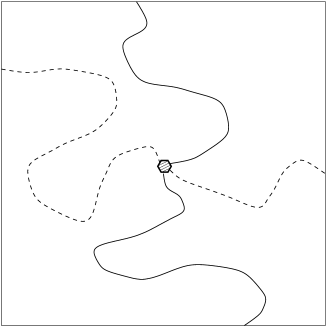
Figure 2: Schematic diagram of a macroscopically pivotal hexagon at the center of four macroscopic arms with alternating color. The full and dashed lines represent paths of white and black hexagons respectively.

The second crucial idea is that in near-critical percolation, as $\lambda$ varies, it is only a special subset of the macroscopically pivotal hexagons that actually have an effect, and these are the ones that need to be marked. To see this, it is best to use the standard coupling for different values of $p$ (and hence different values of $\lambda$) provided by assigning i.i.d. random variables $U_{h}$, uniformly distributed on $(0,1)$, to the hexagons (labelled by $h$) and (for given $\delta$) say that a hexagon $h$ is $\lambda$-white if $U_{h}\leq 1/2+\lambda\delta^{3/4}$. (As remarked in the Introduction, the value $\theta=3/4$ is chosen in order to get nontrivial $\lambda$-dependence in the scaling limit – see [6, 7]). Thus as $\lambda$ varies, a hexagon changes color when $\lambda$ crosses the value $(U_{h}-1/2)\delta^{-3/4}$, and the only hexagons that change color as $\lambda$ varies in $(-\infty,\infty)$ are those where $U_{h}-1/2$ is $O(\delta^{3/4})$ as $\delta\to 0$. The basic ansatz of our approach is that macroscopic changes in connectivity, loops etc. in the scaling limit are those caused by macroscopically pivotal hexagons which change color as $\lambda$ crosses $(U_{h}-1/2)\delta^{-3/4}$. Our marking process marks each such site with the value where it changes from black to white as $\lambda$ increases past that value.

It is known (see [24, 16]) that with an $\varepsilon$-cutoff in the arm-length, there are of order $\delta^{-3/4}$ macroscopically pivotal sites in any bounded region of the plane and thus, as $\lambda$ varies in a bounded interval, there should be $O(1)$ such changing sites. All this should be taken into account automatically by our postulated Poisson marking process, as follows.

Let $P^{\delta}$ be the probability distribution of the collection $X^{\delta}$ of directed cluster boundary loops on the $\delta$-lattice. Conditional on a realization $x^{\delta}$ of $X^{\delta}$, we have denoted by $Y^{\delta}_{\varepsilon}(x^{\delta})$ the collection of $\varepsilon$-macroscopically pivotal hexagons on the $\delta$-lattice. Let us now denote by $\nu^{\delta}_{\varepsilon}$ the (infinite) counting measure on $Y^{\delta}_{\varepsilon}$, rescaled by a factor ${\delta}^{3/4}$, which assigns to a subset $A$ of the plane the measure

$$\nu^{\delta}_{\varepsilon}(A)={\delta}^{3/4}\sum_{y\in A\cap Y^{\delta}_{\varepsilon}(x^{\delta})}1.$$ (1)

It has been proved [10] that $X^{\delta}$ converges in distribution, as $\delta\to 0$, to an $X$ (with distribution $P$) given by (the directed version of) the $SLE_{6}$-based continuum nonsimple loop process of [8, 10]. Two key open problems (which should perhaps be attacked in the opposite order) are (1) to show that the pair $(X^{\delta},\nu^{\delta}_{\varepsilon})$ converges (jointly) in distribution as $\delta\to 0$ to some $(X,\nu_{\varepsilon})$ with $\nu_{\varepsilon}$ (conditional on the realization of $X$) a locally finite measure supported on the double points of $X$ and (2) to understand the nature of $\nu_{\varepsilon}$ (conditional on $X$) in terms of $SLE_{6}$. Note that because of the $\varepsilon$-cutoff, $\nu_{\varepsilon}$ is supported only on either (a) double (touching) points of two loops with each having diameter $\geq\varepsilon$ or (b) double points of single loops such that (as we explain more fully below in Section 4) partitioning the single loop into two “sub-loops” at the double point yields both sub-loops with diameter $\geq\varepsilon$.

The intensity measure of the postulated Poissonian marking process, conditional on a realization of the critical loop process $X$, should be the product measure $\nu_{\varepsilon}\times d\lambda$ where $\nu_{\varepsilon}$ is the just-discussed locally finite measure on double points of $X$ and $d\lambda$ is Lebesgue measure on $(-\infty,\infty)$ for the assignment of a threshold value $\lambda$ to marked points. Thus, there should be a (random) finite number of marked points located in bounded regions of the plane with value $\lambda$ in bounded subsets of $(-\infty,\infty)$. We expect this number to diverge as $\varepsilon\to 0$ (probably even if restricted to those double points where another loop touches a single fixed loop of $X$).

3 $\lambda_{0}$-connectivity

In order to discuss in the next section the near-critical loop process, depending on $\lambda$, we need to discuss in this section the notion of $\lambda_{0}$-white (and $\lambda_{0}$-black) regions and $\lambda_{0}$-white (and $\lambda_{0}$-black) curves in the plane. We begin by discussing the case $\lambda_{0}=0$ corresponding to the critical ($\lambda_{0}=0$) loop process of [8, 10].

A $0$-white region (respectively, $0$-black region) is the union of the image of a counterclockwise $0$-loop $L$ (i.e., one in the critical loop process) with its “interior” less the union of the “interiors” of all its (clockwise) “daughter” loops. Since these loops are nonsimple, the meaning of “interior” needs to be explicated – we define it as follows.

For a counterclockwise (resp., clockwise) loop $L$ represented by the continuous curve $\gamma:[0,1]\longrightarrow{\mathbb{R}}^{2}$ (with $\gamma(0)=\gamma(1)$), the open set ${\mathbb{R}}^{2}\setminus\gamma([0,1])$ is the union of its countably many open, connected components $\Gamma_{0},\Gamma_{1},\Gamma_{2},\ldots$ with $\Gamma_{0}$ unbounded and $\Gamma_{i}$ bounded for $i\geq 1$, with each winding number ${\cal W}(\Gamma_{i})$ of $\gamma$ about $\Gamma_{i}$ (i.e., about any point in $\Gamma_{i}$) for $i\geq 0$ equal to $0$ or $+1$ (resp., $0$ or $-1$). The interior $\text{int}(L)$ of a counterclockwise (resp., clockwise) $L$ is defined as the union of all $\Gamma_{i}$ with $i\geq 1$ and ${\cal W}(\Gamma_{i})=+1$ (resp., ${\cal W}(\Gamma_{i})=-1$). The exterior of $L$ is defined as the union of those $\Gamma_{i}$ (including $\Gamma_{0}$) with ${\cal W}(\Gamma_{i})=0$.

We denote by $L^{*}$ the closure (as a subset of ${\mathbb{R}}^{2}$) of the open set $\text{int}(L)$ and claim that almost surely $L^{*}\setminus\text{int}(L)$ is equal to $\text{tr}(L)$ – the trace of $L$, i.e. $\gamma([0,1])$. (This is not true in general – a counterexample is a curve whose trace is the union of two disjoint circles and a segment joining them, where the points on the segment are double points of the curve – but in our case it follows from the fact that almost surely the trace of a loop $L$ does not “stick to itself.” This, in turn, is a consequence of the Hausdorff dimension of the double points of the trace of an $SLE_{6}$ curve.) The $0$-white (resp., $0$-black) region $\tilde{L}$ defined by the counterclockwise (resp., clockwise) loop $L$ is then $L^{*}\setminus\cup_{L^{\prime}\in{\cal D}(L)}\text{int}(L^{\prime})$ where ${\cal D}(L)$ denotes the countable collection of daughter loops of $L$, or equivalently, $\tilde{L}$ consists of the union of $\text{tr}(L)$ and all the traces $\text{tr}(L^{\prime})$ of the daughter loops of $L$ and all other points $z$ in the plane that are “surrounded” by $L$ but not “surrounded” by any daughter $L^{\prime}$.

Now we can define a $\lambda_{0}$-white curve for $\lambda_{0}\geq 0$ ($\lambda_{0}$-black curves for $\lambda_{0}\leq 0$ are defined similarly) as a curve $\beta$ in the plane whose image is a subset of the union of one or more $0$-white regions and which is not allowed to cross $0$-loops $L$ (although it may touch them) except at $\lambda$-marked sites with $0\leq\lambda\leq\lambda_{0}$. For $\lambda_{0}=0$, this means that the curve stays within a single $0$-white region and does not cross any $0$-loops.

The $\lambda_{0}$-white curves can be used to describe the scaling limits of certain connectivity probabilities for the one-parameter family of near-critical models. For example, the scaling limit of the probability that two disjoint regions of the plane, $D_{1}$ and $D_{2}$, are connected by a white path in the percolation model with $p=1/2+\lambda_{0}\delta^{3/4}$ is given by the probability that there is a $\lambda_{0}$-white curve from $D_{1}$ to $D_{2}$. Analogously, the scaling limit of the probability that in the $\delta$-lattice there is a white crossing of the annulus centered at $z$ with inner radius $r_{1}$ and outer radius $r_{2}$ is the probability that there is a $\lambda_{0}$-white curve crossing the same annulus.

4 $\lambda_{0}$-loop processes

4.1 Construction

In the previous section, we gave a preliminary discussion of $\lambda_{0}$-connectivity. Here we focus on the related notion of $\lambda_{0}$-loops, i.e., the scaling limit as $\delta\to 0$ of the collection of all boundary loops when $p=1/2+\lambda_{0}\delta^{3/4}$. By analogy with the critical ($\lambda_{0}=0$) case and the definition of $0$-white curves there, the guiding idea is to define $\lambda_{0}$-loops in such a way that $\lambda_{0}$-white curves do not cross any $\lambda_{0}$-loop. In order to ensure this, one needs to merge together various $0$-loops and split other $0$-loops, where the merging and splitting takes place at marked double points and the decision to merge or split depends on the value associated to the mark and on $\lambda_{0}$. The result of all this merging and splitting will be the collection of $\lambda_{0}$-loops.

For $\lambda_{0}>0$, the splitting of a $0$-loop (resp., merging of two $0$-loops), caused by a black to white flip, takes place at a marked double point of the loop (resp., where the two loops touch) with $\lambda\in[0,\lambda_{0}]$. There are two types of splitting and two types of merging (see Figure 3):

• the splitting of a counterclockwise loop into an outer counterclockwise and an interior clockwise loop,

• the splitting of a clockwise loop into two adjacent clockwise loops,

• the merging of a counterclockwise loop with the smallest clockwise loop that contains it into a clockwise loop, and

• the merging of two adjacent counterclockwise loops into a counterclockwise loop.

The case $\lambda_{0}<0$ is exactly symmetric to the $\lambda_{0}>0$ case but with splittings and mergings caused by white to black flips.

Figure 3: Schematic diagram representing the different types of splitting and merging caused by a black to white flip. The arrows indicate the orientations of the loops, determined by having white (W) on the left and black (B) on the right.

We point out that things are more complex than they may first appear, based on the previous discussion. This is because the critical loop process is scale invariant and each configuration contains infinitely many loops at all scales, which implies that in implementing the merging/splitting, one needs in principle both a small scale $\varepsilon$-cutoff and a large scale $N$-cutoff. This means that the merging/splitting should first be done only for loops touching a square centered at the origin of side length $N$ and takes place only if both loops involved in the merging or both loops resulting from the splitting have diameter larger than $\varepsilon$. For every $0<\varepsilon<N<\infty$, this ensures that the number of merging and splitting operations is finite. At a later stage, the limits $N\to\infty$ and $\varepsilon\to 0$ should be taken.

4.2 Connectivity Probabilities

The $\lambda_{0}$-loops can be used to describe the scaling limits of certain connectivity probabilities for the one-parameter family of near-critical models. For example, the scaling limit of the probability that two disjoint regions of the plane, $D_{1}$ and $D_{2}$, are connected by a monochromatic path in the percolation model with $p=1/2+\lambda_{0}\delta^{3/4}$ is given by the probability that there is no $\lambda_{0}$-loop with one region in its interior and the other in its exterior (where the interior and exterior are defined for $\lambda_{0}$-loops as they were defined for $0$-loops in Section 3).

To determine whether there is a $\lambda_{0}$-white connecting curve or a $\lambda_{0}$-black one or both, let $L_{i}$ for $i=1,2$ denote the smallest $\lambda_{0}$-loop surrounding $D_{i}$. In the situation we are considering where there is a monochromatic connecting curve, there are three disjoint possibilities (see Figure 4) – either (1) there is a $\lambda_{0}$-loop $L^{\prime}$ touching both $D_{1}$ and $D_{2}$, or (2) there is no such $L^{\prime}$ and $L_{1}=L_{2}$, in which case we define $L=L_{1}=L_{2}$, or (3) there is no such $L^{\prime}$, $L_{1}\neq L_{2}$ and $L_{2}$ surrounds $L_{1}$ (resp., $L_{1}$ surrounds $L_{2}$), in which case we define $L=L_{1}$ (resp., $L=L_{2}$). Note that in case (3), $L_{1}$ touches $D_{2}$ (resp., $L_{2}$ touches $D_{1}$). In case (1), there are both white and black connecting paths; in cases (2) and (3), there is a white but no black connecting path if $L$ is oriented counterclockwise, and otherwise there is a black but no white connecting path.

Figure 4: Examples of monochromatic connections between the disc $D_{1}$ on the left and the disc $D_{2}$ on the right. In (1), there are both white (W) and black (B) connections; in (2) and (3), there is only a white connection.

4.3 Conformal Covariance

The critical loop process has certain conformal invariance properties [10], but one should not expect the $\lambda_{0}$-loop process to be conformally invariant. In fact, for every $\lambda_{0}\neq 0$, the process should possess translation and rotation invariance, but not scale invariance (see, e.g., Section 5 of [7]).

¿From the fact that the $\lambda_{0}$-loop process is the scaling limit of a percolation model with density $p=1/2+\lambda_{0}\delta^{3/4}$, it can be seen that a global dilation by a factor $s$ would map the $\lambda_{0}$-process to a ${\hat{\lambda}_{0}}$-process with ${\hat{\lambda}_{0}}=s^{-3/4}\lambda_{0}$. We will call this property of the one-parameter family of loop processes scale covariance.

Consider now the restriction of a $\lambda_{0}$-loop process to the subdomian $D$ of the plane, and let us assume for simplicity that $D$ is a Jordan domain (i.e., a bounded, simply connected domain whose boundary is a simple loop). This can be obtained by taking the scaling limit inside $D$ (with some care in the choice of “boundary conditions” – we don’t dwell on this issue here, since it is not important for our discussion), and it admits a construction via marked double points analogous to that of the $\lambda_{0}$-loop process in the plane (see Section 4.1).

In the critical case ($\lambda_{0}=0$), if $f:D\to{\hat{D}}$ is a conformal map from $D$ to ${\hat{D}}$, the $0$-loop process inside $D$ is mapped by $f$ to the $0$-loop process inside ${\hat{D}}$ (in distribution). This expresses the conformal invariance of the critical loop process. The previous considerations on the scale covariance of the one-parameter family of loop processes suggest that, in general, a $\lambda_{0}$-loop process in $D$ will be mapped (in distribution) by $f$ to an inhomogeneous ${\hat{\lambda}_{0}}(w)$-loop process in ${\hat{D}}$ where ${\hat{\lambda}_{0}}(w)=|f^{\prime}(z)|^{-3/4}\lambda_{0}$ and $w=f(z)$. We will call this property conformal covariance.

We note that there is no difficulty in interpreting an inhomogeneous loop process within our framework of marked loops. Such a loop process should be simply interpreted as one in which the $\lambda_{0}$ value that determines which marked double points should be used in the splitting/merging procedure (equivalently, can be crossed by a white/black curve) depends on the spatial location of the marks. Such inhomogeneous loop processes would be the scaling limits of spatially inhomogeneous percolation models in which $p=1/2+\lambda\delta^{3/4}$ but with $p$ and $\lambda$ depending on location in the $\delta$-lattice. Conformal covariance is then not just a property of our original one-parameter family of loop processes but rather of this extended family of inhomogeneous loop processes.

Conformal covariance for the extended family means that a $\lambda(z)$-loop process in $D$ is mapped by $f$ to a ${\hat{\lambda}}(w)$-loop process in ${\hat{D}}$ with $\hat{\lambda}(w)=|f^{\prime}(f^{-1}(w))|^{-3/4}\lambda(f^{-1}(w))$. For example, in order to see a homogeneous $\lambda_{0}$-loop process in ${\hat{D}}$, one needs to start with an inhomogeneous $(|f^{\prime}(z)|^{3/4}\lambda_{0})$-loop process in $D$.

4.4 Relation with the Renormalization Group

In view of its scale covariance property, as pointed out by Aizenman [1], the one-parameter family of homogeneous $\lambda_{0}$-loop processes bears an interesting relation to the Renormalization Group picture. Loosely speaking, the action of space dilations can be interpreted as a flow in the space of $\lambda_{0}$-loop models, where a dilation by a factor $s$ corresponds to a change of $\lambda_{0}$ by a factor $s^{-3/4}$.

No general formalism has been found for an exact representation of renormalization group transformations as maps acting in some space, but in this specific example, our framework allows us to make precise the (otherwise vague) meaning of flow in the space of loop models. This is so because all loop models are defined on the same probability space (of critical loops and marks), and the flow simply corresponds to a change of the threshold value $\lambda_{0}$ that determines which marked double points should be used in the splitting/merging procedure (equivalently, can be crossed by a white/black curve). We stress that the key to this interpretation as a flow is the coupling between different loop processes via the marking procedure of Section 2.

5 Dynamical percolation

Our framework allows for the description of a weak limit of dynamical critical percolation [15, 18, 22] under a suitable time scaling (as well as the usual space scaling).

In the dynamical (site) critical percolation model (on the triangular lattice), we have as initial condition a critical configuration of white and black hexagons. The color of each site/hexagon evolves by flipping successively to the other color according to a rate 1 Poisson process, independent of those of the other sites.

We scale space, as previously, by $\delta$ and time by $\delta^{-\theta}$ with $\theta=3/4$ (so that the rate of the Poisson process slows down by a factor $\delta^{3/4}$ – i.e., one unit of rescaled time corresponds to $\delta^{3/4}$ units in the original lattice model). The same considerations as in Section 2 lead to the ansatz that, under this combined scaling, only the flips of macroscopically pivotal hexagons are relevant. For an eventual rigorous construction, we may also need to implement a cutoff procedure on small and large scales like the one described in Section 4.1.

As discussed in Section 2, the set of macroscopically pivotal hexagons between two almost-touching macroscopic (large) loops (as well as those of a single almost-self-touching loop – with the usual proviso that upon flipping any one of these hexagons, there should result two (large) macroscopic loops) has cardinality of the order of $\delta^{-3/4}$. Thus the choice of $\theta=3/4$ for the time variable scaling implies that, in the limit $\delta\to 0$, we should see the following dynamics on the set of double points of the (critical) continuum loop process. Consider the double points between two given loops (or alternatively from a single loop) in the initial configuration of (critical) loops. The color flipping of the (macroscopically pivotal) hexagons at the discrete level will correspond in the scaling limit to a process of marking double points in the continuum. The marking takes place according to a Poisson process in space-time whose intensity measure is $\nu_{\varepsilon}\times dt$ with $\nu_{\varepsilon}$ the measure on the set of double points in question described in Section 2. (Note that eventually, the limit $\varepsilon\to 0$ is taken.) At an event of the Poisson process, a mark is assigned to a double point at a certain time. The effect is essentially the same as that of the marking in the static model: when a mark appears at a double point of two touching loops, then those loops merge at the marked point; if it is a single loop touching itself at that point, then after the time of the mark we have two loops touching at that point (see Section 4 and Figure 3 there).

We remark that this dynamics can be realized using the static marking of the critical loops, as described in Section 2. Consider the same set of double points of two given loops or a single loop of the initial configuration of (critical) loops as above, but this time we mark this set with the static $\lambda$ marks as in Section 2. The dynamics is a function of the loops and static marks as follows. As in the previous description, (dynamical) marks will appear at certain times at certain double points. The set of those spatial points where this takes place is exactly the set of double points with the static $\lambda$ marks. It remains to say at which time a dynamical mark appears at a given such site: the answer is simply that it appears at a site with the static mark $\lambda_{0}$ at time $|\lambda_{0}|$.

As noted in [21], the dynamical percolation scaling limit should not be expected to be conformally invariant. However, its construction in terms of the static marks shows that it must possess the same conformal covariance as the family of loop processes of Section 4.3, with the role of $\lambda$ played by time $t$. This means that if $f:D\to{\hat{D}}$ is a conformal map from $D$ to ${\hat{D}}$, the dynamical percolation scaling limit inside $D$ at time $t_{0}$ is mapped (in distribution) by $f$ to a dynamical percolation scaling limit in ${\hat{D}}$ at a spatially dependent time ${\hat{t}}_{0}(w)$ given by ${\hat{t}}_{0}(w)=|f^{\prime}(z)|^{-3/4}t_{0}$, where $w=f(z)$. This gives a “relativistic” framework where time is not “absolute,” and suggests a positive answer to a question posed by Schramm in [21].

6 $\lambda_{0}$-exploration path

Take the hexagonal lattice embedded in the plane so that one of its axes of symmetry is parallel to the $y$-axis. Consider the set of hexagons that intersect the upper half-plane $\mathbb{H}$ and induce two infinite clusters by coloring the hexagons touching the $x$-axis white if they lie to the left of a given hexagon and black otherwise. The other hexagons in $\mathbb{H}$ are colored white or black independently, with equal probability. With probability one, there are exactly two infinite clusters, one white and one black. The critical percolation exploration path in $\mathbb{H}$ is the interface separating the infinite white cluster from the infinite black cluster.

In a seminal paper [20], Schramm conjectured that in the scaling limit this critical percolation exploration path converges in distribution to (the trace of) chordal $SLE_{6}$. Shortly thereafter, a crucial part of the connection between the exploration path and $SLE_{6}$ was made rigorous by Smirnov’s proof [23] of convergence of crossing probabilities to Cardy’s formula [12]. Smirnov [23] also proposed a strategy to use his Cardy formula results to prove Schramm’s complete conjecture. A detailed proof of the Schramm conjecture [9, 11] followed a few years later.

The (full) scaling limit of the critical half-plane percolation model with the white/black boundary conditions described above gives a half-plane critical loop process together with a continuous, infinite curve $\gamma$ distributed like the trace of chordal $SLE_{6}$ (in the upper half-plane). $\gamma$ does not cross any loops but touches infinitely many of them (and indeed is constructed by piecing together segments of the loops, as discussed in [9, 10]).

Consider now a percolation model in the upper half-plane where, as before, the hexagons touching the $x$-axis are colored white if they are to the left of a given hexagon and black otherwise, but the remaining hexagons are colored white with probability $p=1/2+\lambda_{0}\delta^{3/4}$ and black otherwise. For $\delta$ fixed and $\lambda_{0}$ positive (resp., negative), we are in the white (resp., black) supercritical phase. However, the choice of boundary conditions implies that, together with an (almost surely unique) infinite white (resp., black) cluster, there is also an (almost surely unique) infinite black (resp., white) cluster. The $\lambda_{0}$-percolation exploration path (for lattice spacing $\delta$) in the upper half-plane is the interface separating the infinite white cluster from the infinite black cluster of this percolation model.

It is natural to conjecture that, as $\delta\to 0$, the scaling limit of the discrete $\lambda_{0}$-exploration path converges in distribution to a continuous path, and further that this continuum $\lambda_{0}$-exploration path can be obtained from the scaling limit of the critical exploration path (i.e., chordal $SLE_{6}$) and the half-plane critical loops by means of the marking of double points discussed in Section 2, together with a suitably adapted version of the splitting and merging procedure described in Section 4.

The splitting and merging of loops is analogous to that described in Section 4; the novelty here consists in the self-touching of the exploration path and in the “interaction” between the exploration path and the loops it touches. The resulting double points should be marked as described in Section 2, so that at a marked double point, a critical loop can merge into the exploration path or a new $\lambda_{0}$-loop can be created by splitting off from the exploration path.

For $\lambda_{0}>0$, the mergings and splittings are caused by black to white flips of pivotal hexagons, and in the scaling limit correspond to the following two situations:

• a counterclockwise critical loop touching the critical exploration path at a marked double point can merge with it, becoming part of the $\lambda_{0}$-path, or

• the critical exploration path can split at a marked (self-touching) double point into a “shorter” path and a clockwise $\lambda_{0}$-loop touching each other at the marked double point.

The case $\lambda_{0}<0$ is of course symmetric to the one described here but with splittings and mergings caused by white to black flips.

Once again, as already explained in Section 4, things are more complex than they may appear from the above description, and one needs in principle both a small scale $\varepsilon$-cutoff and a large scale $N$-cutoff (see Section 4.1 for a discussion of this point).

The scaling limit of the $\lambda_{0}$-exploration path for $\lambda_{0}\neq 0$ should not be expected to be scale invariant. However, its construction in terms of splitting and merging of loops at marked double points as described above shows that it should possess a scale covariance property (see Section 4.3).

To further explore how the scaling limit of the $\lambda_{0}$-exploration path should change under conformal transformations, let us consider the $\lambda_{0}$-exploration path inside a Jordan domain. Given a Jordan domain $D$ with two distinct points $a,b$ on its boundary $\partial D$, one can define the $\lambda_{0}$-exploration path inside $D$ from $a$ to $b$ just like the $\lambda_{0}$-exploration path in $\mathbb{H}$ from $0$ to $\infty$. More precisely, one has to choose appropriate boundary conditions (say, white on the counterclockwise arc $\overline{ba}$ and black on the counterclockwise arc $\overline{ab}$) and then consider the unique interface between the white cluster touching the counterclockwise arc $\overline{ba}$ and the black cluster touching the counterclockwise arc $\overline{ab}$.

It follows from the considerations of Section 4.3 that if $f:D\to{\hat{D}}$ is a conformal map from $D$ to ${\hat{D}}$, the scaling limit of the $\lambda_{0}$-exploration path inside $D$ is mapped by $f$ to a curve ${\hat{\gamma}}$ in ${\hat{D}}$ from ${\hat{a}}=f(a)$ to ${\hat{b}}=f(b)$ whose distribution can be obtained in the following way. Consider the full scaling limit inside ${\hat{D}}$ with white/black boundary conditions, corresponding to an $SLE_{6}$ path $\gamma$ from ${\hat{a}}$ to ${\hat{b}}$ and a countable number of critical loops. Then ${\hat{\gamma}}$ is distributed like the path obtained from $\gamma$ after applying to it the splitting/merging procedure described above with a spatially dependent threshold value given at $w=f(z)$ by $|f^{\prime}(z)|^{-3/4}\lambda_{0}$.

7 Minimal Spanning Trees and plane-filling curves

In this section, we propose a construction of the scaling limit of the discrete minimal spanning tree (MST), using our framework of continuum nonsimple loops and marked double points. For an interesting discussion of universality properties of the MST in two (and higher) dimensions, see [19]. The discrete MST is most easily defined on the square lattice, so in this section we focus on bond percolation on ${\mathbb{Z}}^{2}$. For each nearest neighbor bond (or edge) $b$, let $U_{b}$ be a uniform $(0,1)$ random variable with the $U_{b}$’s independent. This provides a standard coupling of bond percolation models for all values $p$ of the probability that a bond $b$ is open by saying that $b$ is $p$-open if $U_{b}\leq p$. One then defines the minimal spanning tree in, say, an $N\times N$ square $\Lambda_{N}$ centered at the origin, with free boundary conditions, as the spanning tree in $\delta{\mathbb{Z}}^{2}\cap\Lambda_{N}$ with the minimum value of $\sum_{b}U_{b}$ summed over $b$’s in the tree. It is known, based on the relation to invasion percolation, that there is with probability one a single limiting tree as $N\to\infty$ (see [13, 5, 17]). We will denote this tree on the $\delta$-lattice, $\delta{\mathbb{Z}}^{2}$, by $T_{\delta}$.

The purpose of this section is to describe the putative scaling limit (in distribution) of $T_{\delta}$ as $\delta\to 0$, in terms of the critical $0$-loop process and our $\lambda$-marked double points. Our description uses a minimax construction in the continuum which is a natural analogue of a well-known one on the lattice (see, e.g., [5] and references therein). We ignore differences between bond percolation on the square lattice and site percolation on the triangular lattice in the belief that they have no effect on the continuum scaling limit; in particular we will use “white” and “open” interchangeably.

Once the (lattice) MST has been defined, a dual tree on the dual lattice arises naturally as the unique spanning tree of the dual lattice which uses only those dual bonds that are perpendicular to bonds that do not belong to the MST. More precisely, given a minimal spanning tree $T_{\delta}^{N}$ in $\delta{\mathbb{Z}}^{2}\cap\Lambda_{N}$ with free boundary conditions, the dual tree is a spanning tree $\tilde{T}_{\delta}^{N}$ on (a portion of) the dual lattice $\delta[{\mathbb{Z}}^{2}+(1/2,1/2)]$ with wired boundary conditions, i.e., with all the dual sites in the boundary (of that portion of the dual lattice) identified and treated as a single site. The edges of the dual tree $\tilde{T}_{\delta}^{N}$ cross only edges of ${\mathbb{Z}}^{2}$ that do not belong to $T_{\delta}^{N}$. The dual tree is distributed like a minimal spanning tree (on the dual lattice) with wired boundary conditions. It can be shown that the $N\to\infty$ limits of the minimal spanning tree exist for both free and wired boundary conditions and moreover that the two limits coincide (see [13, 5, 17]). The spanning tree $T_{\delta}^{N}$ and its dual $\tilde{T}_{\delta}^{N}$ together define a “lattice-filling” curve $\pi_{\delta}^{N}$ as the curve that separates them (see Figure 5). With this choice of boundary conditions, $\pi_{\delta}^{N}$ is actually a lattice-filling loop. In the limit $N\to\infty$, we drop the $N$ superscript.

Figure 5: Examples of a spanning tree (heavy line) with free boundary conditions, its dual (heavy broken line) and the “lattice filling” curve between them.

The MST $T_{\delta}$ can be decomposed into a forest $\cal F$ ($={\cal F}_{\delta}$) whose connected components are the minimal spanning trees of the individual critical ($p=1/2$) open clusters, such that each “cluster tree” uses only bonds from a single open cluster (including singleton site clusters when that site in the lattice has all four of its touching edges closed), plus the set $\cal R$ of all the remaining bonds minimally connecting all those cluster trees. If we consider the individual open clusters as the vertices of a graph $\mathbb{G}$ whose edges are the bonds connecting distinct open clusters (and we may focus on those bonds with the smallest value of $U_{b}$ for each adjacent pair of open clusters), we can define a minimal spanning tree for $\mathbb{G}$. Combining this minimal $\mathbb{G}$-spanning tree and the forest $\cal F$ gives back the usual MST for $\delta{\mathbb{Z}}^{2}$.

In the scaling limit, we may consider the continuum MST as the limiting set of paths within the tree (see [4] for a general discussion of continuum scaling limits of trees, which takes a somewhat different point of view). In order to define this tree, it is enough to describe the (unique, with probability one) tree path between any two given deterministic points in ${\mathbb{R}}^{2}$. However, it will be more convenient to describe the continuum tree path between pairs of (non-deterministic) points, $z_{1},z_{2}$, such that each is contained in a continuum $0$-white region. Since such points are dense in ${\mathbb{R}}^{2}$, one should obtain from these the paths between all pairs of points, including deterministic ones.

For this purpose, we will use the idea of $\lambda$-connectivity introduced in Section 3. Any two points $z_{1},z_{2}$ contained in continuum $0$-white (open) regions (of the critical model) should be $\lambda$-connected for some large enough value $\lambda<\infty$. To find the tree path between $z_{1}$ and $z_{2}$, we start decreasing $\lambda$ from $+\infty$ until it reaches a value $\lambda_{1}$ below which $z_{1}$ and $z_{2}$ are not $\lambda$-connected. $\lambda_{1}$ is the smallest $\lambda$ for which $z_{1}$ and $z_{2}$ are $\lambda$-connected and furthermore $\lambda_{1}$ should be the value of a unique marked point $\zeta_{1}$ on all $\lambda_{1}$-paths from $z_{1}$ to $z_{2}$. We then reduce $\lambda$ below $\lambda_{1}$ to a value $\lambda_{2}$ below which either $z_{1}$ or $z_{2}$ is disconnected from $\zeta_{1}$. This will give us a new marked point $\zeta_{2}$ labelled with a $\lambda$ equal to $\lambda_{2}$. The procedure continues iteratively until the points $\zeta_{i}$ fill in a continuous path between $z_{1}$ and $z_{2}$.

The procedure outlined above is the continuum version of a standard minimax algorithm (see, e.g., [5] and references therein) to construct the minimal spanning tree on ${\mathbb{Z}}^{2}$ (using uniform $(0,1)$ bond variables) where one looks at the minimum over all paths from $z_{1}$ to $z_{2}$ of $\max_{b\in\text{path}}U_{b}$ to get a particular bond, and then the procedure is repeated iteratively as above.

We note that the minimax value of $\lambda$ for the connection between points in two different $0$-white (open) regions will be positive, while the minimax value of $\lambda$ for the connection between points in the same $0$-white (open) region will be negative. The minimal spanning tree path between two points in the same continuum $0$-white/open region is obtained by decreasing $\lambda$ from $0$ towards $-\infty$, and the minimax points will be either double points of the counterclockwise $0$-loop surrounding the cluster or points in the interior of that counterclockwise $0$-loop where two clockwise daughter $0$-loops touch each other or points where one such daughter loop touches the mother $0$-loop.

We remark that we have presented our continuum minimax construction of the continuum MST in a relatively simple version that does not use any cutoffs (like those discussed in Section 4.1). Even if such cutoffs turn out to be needed, the resulting construction should still be feasible within our framework of loops and marked double points.

The restrictions to the $0$-white/open regions of the continuum tree paths correspond to the scaling limit of the forest $\cal F$ ($={\cal F}_{\delta}$), while the minimal $\mathbb{G}$-spanning tree converges in the scaling limit to a minimal “cluster connecting tree,” i.e., a minimal spanning tree in the “graph” whose vertices are the continuum $0$-white regions and whose edges are the marked double points between them.

The scaling limit of the lattice-filling curve separating the MST and its dual tree gives a continuous plane-filling curve closely related to the $\lambda$-loops. To see this, let us explain how to go from the plane-filling curve to the $\lambda_{0}$-loops for some $\lambda_{0}>0$. First of all, we give an orientation to the lattice-filling and plane-filling curve so that the MST is to the left as one follows the oriented curve. Next, we note that the double points of the space-filling curve are at marked points and are of two types, depending on whether they occur at clockwise double points or at counterclockwise double points – i.e., ones where the oriented loop formed by the curve between the first and second times it touches the double point is clockwise or counterclockwise. With this in mind, roughly speaking one proceeds as follows. Starting from a marked counterclockwise double point with $\lambda>\lambda_{0}$ (resp., a clockwise double point with $\lambda<\lambda_{0}$), one begins by following the plane-filling curve in the counterclockwise direction (resp., the clockwise direction), taking shortcuts at every clockwise marked point with $\lambda<\lambda_{0}$ and at every counterclockwise marked point with $\lambda>\lambda_{0}$, until one returns to the starting marked point. This gives a $\lambda_{0}$-loop.

To actually carry this out, one needs to take a double $(\varepsilon,K)$ cutoff, meaning that the marked points with $\lambda<-K$ or $\lambda>K$ are ignored and moreover a shortcut is taken only if the diameter of the detour is at least $\varepsilon$. The cutoff is removed by letting first $K\to\infty$ and then $\varepsilon\to 0$.

To conclude this section, we consider the scale and conformal invariance properties of the continuum MST. It is not known for sure whether or not the scaling limit of the MST is conformally invariant and there does not seem to be general agreement on what to conjecture (but a recent numerical study [26] suggests that the continuum MST is not conformally invariant).

Consider the scaling limit of the MST inside the Jordan domain $D$, and let $f:D\to{\hat{D}}$ be a conformal map from $D$ to anther Jordan domain ${\hat{D}}$. As we explained above, the lattice MST can be decomposed into a forest $\cal F$ ($={\cal F}_{\delta}$) and a minimal $\mathbb{G}$-spanning tree, where the latter is conjectured to converge in the scaling limit to a minimal spanning tree in the “graph” whose vertices are the continuum $0$-white regions and whose edges are the (minimal) marked double points between them. The construction of the continuum $0$-white regions from the (critical) $0$-loops suggests that they should be conformally invariant. Therefore the image of the set of continuum $0$-white regions of $D$ under $f$ should be distributed like the set of continuum $0$-white regions of ${\hat{D}}$. However, from the considerations in Section 4.3, we know that if we transport to ${\hat{D}}$ the $\lambda$-marks associated to the double points in $D$, the distribution of the $\lambda$-marks that we obtain in ${\hat{D}}$ is not the correct one, conditioned on the loops (and their double points); i.e., it is not the one that would have been obtained by carrying out the marking procedure of Section 2 in ${\hat{D}}$. In fact, as explained in Section 4.3, in order to get the correct $\lambda_{0}$-loops in ${\hat{D}}$ from the loops obtained by mapping the critical loops from $D$, one needs to rescale the $\lambda$-marks of double points in $D$, typically in an inhomogeneous way. This seems to suggest that the image under $f$ of the continuum MST in $D$ is typically not distributed like a continuum MST in ${\hat{D}}$, and therefore that the scaling limit of the MST is not conformally invariant.

Note, however, that if the conformal transformation is a simple dilation, the $\lambda$-marks need to be rescaled in a homogeneous way, so that the distributions of the continuum $\mathbb{G}$-spanning trees obtained from the marks before and after the rescaling should coincide, suggesting that the minimal spanning tree is scale invariant (in distribution).

Another possible way to check the conformal invariance of the continuum MST is by considering the distribution of the tree path between two given points, $z_{1},z_{2}\in D$. As explained above, this path can presumably be obtained via a minimax algorithm that uses the marked double points in $D$ and their $\lambda$-marks. The image under $f:D\to{\hat{D}}$ of the tree path between $z_{1}$ and $z_{2}$ is clearly the result of an identical minimax algorithm in ${\hat{D}}$ using the $\lambda$-marks carried over from $D$. On the other hand, the tree path in ${\hat{D}}$ between $f(z_{1})$ and $f(z_{2})$ is obtained by the same minimax procedure using “fresh” $\lambda$-marks, assigned independently of the $\lambda$-marks in $D$. But since a conformal map from $D$ to ${\hat{D}}$ typically changes the distribution of the $\lambda$-marks in an inhomogeneous way, it seems likely that the image under $f$ of the tree path in $D$ between $z_{1}$ and $z_{2}$ will not be distributed like the tree path in ${\hat{D}}$ between $f(z_{1})$ and $f(z_{2})$. This suggests once again that the scaling limit of the minimal spanning tree is not conformally invariant.

8 Invasion Percolation

We now turn to the scaling limit of (bond) invasion percolation on ${\mathbb{Z}}^{2}$. This also has a description in terms of the continuum marked loop model as argued below.

The discrete model is as follows [25, 13]. Each (nearest neighbor) bond of ${\mathbb{Z}}^{2}$ is assigned a positive continuous random variable (say, uniformly distributed in $(0,1)$) – called the resistance of the bond – independent from those of the other bonds. Starting at a given site (say, the origin), sites are successively invaded, one at a time, along bonds of least resistance among those connecting previously invaded sites to uninvaded sites. The invaded cluster (of the origin, at time infinity) is the tree graph whose sites are all those eventually invaded by this procedure and whose edges are all the bonds which were invaded to reach these sites.

Let us color white the bonds with resistance smaller than $1/2$, and color black the remaining bonds; let us also color the dual bonds with the same color of the respective primal ones. We then have that the set of white bonds form a critical percolation model. Consider now the family of clusters of sites connected by the white bonds of this percolation model (all of which are almost surely finite) and their boundaries of black dual circuits. It is clear from the rules of invasion that, before crossing any such circuit (along any of its primal black bonds), all the sites in the respective white cluster are invaded, after which the invasion proceeds using the bonds of least resistance at the boundaries of the white clusters in question. After rescaling space by a small $\delta$, only macroscopic white clusters/black circuits are relevant, and, following our ansatz and the rules of invasion, only macroscopically pivotal bonds on black macroscopic circuits where two macroscopic white clusters (almost) touch and which have resistance $1/2+\lambda\delta^{3/4}$, $\lambda>0$, are relevant.

In the scaling limit, the following picture then emerges. Given the system of critical counterclockwise loops along with their (positive) $\lambda$-marks, suppose that a given set of $0$-white (critical) regions (whose boundaries touch two by two) has been invaded thus far. The invasion can be started from the smallest counterclockwise loop surrounding the ball of radius $\varepsilon$ centered at the origin, where eventually $\varepsilon\to 0$.) The invasion thence proceeds by next incorporating the not currently invaded $0$-white region whose outer boundary has the least $\lambda$ among all of the marked double points between invaded and not yet invaded clusters. The result of the invasion (after infinite time) can then be seen as a graph whose sites are continuum $0$-white regions and whose edges are certain of the marked double points between them. Here, as before, we may need a cutoff procedure to insure that the above least $\lambda$ value is realized.

To conclude this section, we briefly explain the connection between minimal spanning trees and invasion percolation. As argued in the previous section, the $\delta$-lattice MST can be decomposed into a forest $\cal F$ of minimal spanning trees such that each tree uses only bonds from a single open cluster, plus the set $\cal R$ of all the remaining edges connecting those trees. Each tree in $\cal F$ is obtained by doing invasion percolation “with trapping” inside an open cluster, that is, starting at a random site $x_{0}$ of the cluster, the bond $b$ incident on $x_{0}$ with the smallest $U_{b}$ and the other site $x_{1}$ that $b$ is incident on are invaded, then the procedure is repeated by looking at all the non-invaded bonds incident on $x_{0}$ and $x_{1}$, and so on, with the proviso that a bond is not invaded if it is incident on two sites that are both already invaded. The procedure stops when all the sites of the clusters have been invaded, and the above proviso ensures that the invaded bonds form a tree. It is easy to see that the result is independent of the starting site $x_{0}$ and that the tree obtained is the minimal spanning tree for the given cluster. A similar invasion algorithm can be used to obtain the bonds in $\cal R$ by considering the open clusters as the vertices of a graph $\mathbb{G}$ whose edges are the ${\mathbb{Z}}^{2}$-paths between them, and doing invasion percolation in $\mathbb{G}$.

Acknowledgements. The research of the authors was supported in part by the following sources: for F. C., a Marie Curie Intra-European Fellowship under contract MEIF-CT-2003-500740 and a Veni grant of the Dutch Science Organization (NWO); for L. R. G. F., FAPESP project no. 04/07276-2 and CNPq projects no. 307978/2004-4 and 475833/2003-1; for C. M. N., grant DMS-01-04278 of the U.S. NSF. This paper has benefitted from the hospitality shown to various of the authors at a number of venues where the research and writing took place, including the Courant Institute of Mathematical Sciences, the Ninth Brazilian School of Probability at Maresias Beach, Instituto de Matemática e Estatística - USP, and Vrije Universiteit Amsterdam. The authors thank Marco Isopi and Jeff Steif for useful discussions.

References

- [1] M. Aizenman, Scaling limit for the incipient spanning clusters, in Mathematics of Multiscale Materials; the IMA Volumes in Mathematics and its Applications (K. Golden, G. Grimmett, R. James, G. Milton and P. Sen, eds.), Springer (1998).
- [2] M. Aizenman, Continuum limits for critical percolation and other stochastic geometric models, in XII Int. Cong. Math. Phys. (ICMP ’97, Brisbane), Internat. Press, Cambridge, MA (1999).
- [3] M. Aizenman and A. Burchard, Hölder regularity and dimension bounds for random curves, Duke Math. J. 99, 419–453 (1999).
- [4] M. Aizenman, A. Burchard, C. M. Newman, D. Wilson, Scaling Limits for Minimal and Random Spanning Trees in Two Dimensions, Random Struct. Alg. 15, 319–367 (1999).
- [5] K. S. Alexander, Percolation and Minimal Spanning Forests in Infinite Graphs, Ann. Probab. 23, 87–104 (1995).
- [6] C. Borgs, J. Chayes, H. Kesten, J. Spencer, The Birth of the Infinite Cluster: Finite-Size Scaling in Percolation, Comm. Math. Phys. 224, 153–204 (2001).
- [7] F. Camia, L. R. G. Fontes, C. M. Newman, The Scaling Limit Geometry of Near-Critical 2D Percolation, J. Stat. Phys., to appear (2006).
- [8] F. Camia and C. M. Newman, Continuum Nonsimple Loops and 2D Critical Percolation, J. Stat. Phys. 116, 157–173 (2004).
- [9] F. Camia and C. M. Newman, The full scaling limit of two-dimensional critical percolation, available at arXiv:math.PR/0504036 (2005), including a main part corresponding to [10] and a long appendix roughly corresponding to [11].
- [10] F. Camia and C. M. Newman, The full scaling limit of two-dimensional critical percolation, submitted (2005).
- [11] F. Camia and C. M. Newman, Critical Percolation Exploration Path and : a Proof of Convergence, in preparation (2006).
- [12] J. L. Cardy, Critical percolation in finite geometries, J. Phys. A 25, L201–L206 (1992).
- [13] J. T. Chayes, L. Chayes, C. M. Newman, The Stochastic Geometry of Invasion Percolation, Comm. Math. Phys. 101, 383–407 (1985).
- [14] L. R. G. Fontes, M. Isopi, C. M. Newman, K. Ravishankar, Coarsening, Nucleation, and the Marked Brownian Web, Ann. Inst. H. Poincaré (B), Prob. and Stat. 42, 37–60 (2006).
- [15] O. Häggström, Y. Peres, J. E. Steif, Dynamical percolation, Ann. Inst. H. Poincaré Probab. Statist. 33, 497–528 (1997).
- [16] G. J. Morrow and Y. Zhang, The sizes of the pioneering, lowest crossing and pivotal sites in critical percolation on the triangular lattice, Ann. Appl. Probab. 15, 1832–1886 (2005).
- [17] C. M. Newman and D. L. Stein, Ground State Structure in a Highly Disordered Spin Glass Model, J. Stat. Phys. 82, 1113–1132 (1996).
- [18] Y. Peres, J. E. Steif, The number of infinite clusters in dynamical percolation, Probab. Theory Related Fields 111, 141–165 (1998).
- [19] N. Read, Minimal spanning trees and random resistor networks in dimensions, Phys. Rev. E 72, 036114-1–036114-17 (2005).
- [20] O. Schramm, Scaling limits of loop-erased random walks and uniform spanning trees, Israel J. Math. 118, 221–288 (2000).
- [21] O. Schramm, Conformally invariant scaling limits: an overview and a collection of problems, preprint math.PR/0602151 (2006).
- [22] O. Schramm, J. E. Steif, Quantitative noise sensitivity and exceptional times for percolation, preprint math.PR/0504586 (2005).
- [23] S. Smirnov, Critical percolation in the plane: Conformal invariance, Cardy’s formula, scaling limits, C. R. Acad. Sci. Paris 333, 239–244 (2001).
- [24] S. Smirnov and W. Werner, Critical exponents for two-dimensional percolation, Math. Rev. Lett. 8, 729–744 (2001).
- [25] D. Wilkinson and J. F. Willemsen, Invasion percolation: A new form of percolation theory, J. Phys. A 16, 3365–3376 (1983).
- [26] D. Wilson, private communication (2005).