Phonon-mediated tuning of instabilities in the Hubbard model at half-filling

Abstract

We obtain the phase diagram of the half-filled two-dimensional Hubbard model on a square lattice in the presence of Einstein phonons. We find that the interplay between the instantaneous electron-electron repulsion and electron-phonon interaction leads to new phases. In particular, a d${}_{x^{2}-y^{2}}$-wave superconducting phase emerges when both anisotropic phonons and repulsive Hubbard interaction are present. For large electron-phonon couplings, charge-density-wave and s-wave superconducting regions also appear in the phase diagram, and the widths of these regions are strongly dependent on the phonon frequency, indicating that retardation effects play an important role. Since at half-filling the Fermi surface is nested, spin-density-wave is recovered when the repulsive interaction dominates. We employ a functional multiscale renormalization-group methodSWTsai2005 that includes both electron-electron and electron-phonon interactions, and take retardation effects fully into account.

I Introduction

The renormalization-group (RG) approach to interacting fermionsShankar1994 has recently been extended to include the study of interacting fermions coupled to bosonic modes, such as phononsSWTsai2005 . Experimental evidence indicates that in many strongly correlated systems, such as organic conductors and superconductorsorganics , cupratescuprates1 ; cuprates2 , cobaltatescobaltates , and conducting polymerspolymers , both electron-electron interactions and phonons may play an important role. Also, recent advances in the field of cold atoms have made possible the creation of fermion-boson mixtures on artificial lattices. In these mixtures the fermions interact through instantaneous on-site repulsion, and when the bosonic atoms condense, there is an additional retarded attractive interaction mediated by the fluctuations of the bosonic condensate; a scenario similar to that of electron and phonon interaction in solid state systemsMatley2006 . The physics of the interplay between the repulsive electron-electron (e-e) and attractive electron-phonon (e-ph) interaction is not well understood and fundamental questions arise that include a full understanding of retardation effects and whether competition/cooperation between these interactions can lead to new phases.

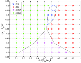
Figure 1: (Color online) Phase diagram for Einstein phonons of frequency $\omega_{E}=1.0$. Four phases involving antiferromagnetism (sSDW) (purple squares), charge density wave (sCDW) (green stars) and s-wave (sSC) (blue circles) and d-wave (dSC) (red rhombs) superconductivity compete in the vicinity where the average phononic strength $\bar{\lambda}$ approaches the bare on-site repulsion $u_{0}=0.5$. The lines distinguishing the different domains are guides to the eye.

One of the most extensively studied model is the two-dimensional repulsive Hubbard modelSchulz1987 ; Hubbard-RG ; Gonzalez1996 ; Senechal2005 , which in the absence of phonons and at half-filling becomes an antiferromagnet due to nesting in the Fermi surface (FS) which drives an s-wave spin density wave (sSDW) instability. In the presence of isotropic phonons and in the strongly coupled regime, it has been shown that the s-wave charge density wave instability dominates over antiferromagnetism and coexists with s-wave superconductivity (sSC)Berger1995 . When anisotropic phonons are present and full retardation is taken into account the phase diagram in parameter space associated with this model is summarized in Fig. (1), which reproduces the usual sSDW and sCDW instabilities but additionally a d${}_{x^{2}-y^{2}}$-wave superconducting phase (dSC). Therefore, in this work we show that this dSC phase which appears at half-filling, is a result of cooperation between the two interactions. We stress that the role of the phonons goes beyond simply creating an effective attractive force between the electrons. Retardation plays a crucial role in generating the new phases, and the size of each region depends on the phonon frequency. This model can also be used to study various other systems where the e-ph interaction is present such as the quasi-2D $\kappa$-(BEDT-TTF)₂-X materials, which are stoichiometric with a fixed density of one electron per BEDT-TTF dimerkappa , or as we mentioned in the beginning, for fermion-boson optical lattice mixtures (where there is experimental control on the number of fermions per lattice point) deep in the bosonic condensate phase. This study is by no means complete in its results since it is limited to the weak coupling regime but is intended to chart the vast phase space of these type of systems with some preliminary results that will help arrange the important underlying physics and contribute to a better understanding of the competition and cooperation between the interactions involved.

This paper is organized as follows. In section II we introduce the theoretical model and the RG method of analysis we employ. In section III we provide our results and draw the phase diagrams associated with the different orders in the system. In section IV we discuss the summary and the basic physics our work has highlighted and finally in the appendix we provide more details for the RG flow of the couplings and susceptibilities for the reader that is interested on the theoretical details.

II Theoretical Model

The approach we employ in this study is based on a general RG analysis of a system of electrons recently expanded to involve the coupling of the electrons with phonons as wellSWTsai2005 . We use a generic model of electrons on a Hubbard lattice at half-filling interacting through the repulsive Coulomb interaction and being isotropically and anisotropically coupled to dispersionless bosonic excitations (Einstein phonons). The Hamiltonian associated with this type of system is

$$H\!\!\! = \!\!\!\sum_{{\mathbf{k}},\sigma}\xi_{{\mathbf{k}}}c_{{\mathbf{k}},\sigma}^{\dagger}c_{{\mathbf{k}},\sigma}+\!\!\!\sum_{{\mathbf{k}}_{1},{\mathbf{k}}_{2},{\mathbf{k}}_{3}}\!\!\sum_{\sigma}u_{0}c_{{\mathbf{k}}_{3},\sigma}^{\dagger}c_{{\mathbf{k}}_{4},-\sigma}^{\dagger}c_{{\mathbf{k}}_{2},-\sigma}c_{{\mathbf{k}}_{1},\sigma}$$ (1)

$$+\omega_{E}\sum_{{\mathbf{q}}}b_{{\mathbf{q}}}^{\dagger}b_{{\mathbf{q}}}+\sum_{{\mathbf{q}},{\mathbf{k}}}g(q)c_{{\mathbf{k}}+{\mathbf{q}},\sigma}^{\dagger}c_{{\mathbf{k}},\sigma}(b_{{\mathbf{q}}}+b_{-{\mathbf{q}}})$$

where $c_{{\mathbf{k}},\sigma}^{\dagger}$($c_{{\mathbf{k}},\sigma}$) is the creation (annihilation) operator of an electron with momentum ${\mathbf{k}}$ and spin $\sigma$, and $b_{{\mathbf{q}}}^{\dagger}$ ($b_{{\mathbf{q}}}$) is the corresponding creation (annihilation) operator of a phonon with momentum ${\mathbf{q}}$. Also, $\xi_{{\mathbf{k}}}=-2t(\cos k_{x}+\cos k_{y})$ is the non-interacting electron energy at half-filling, $\omega_{E}$ is the Einstein frequency, $u_{0}$ is the e-e on-site repulsion, while the e-ph coupling $g(q)$ is taken to be momentum dependent. Momentum conservation (up to reciprocal lattice vectors) implies ${\mathbf{k}}_{4}={\mathbf{k}}_{1}+{\mathbf{k}}_{2}-{\mathbf{k}}_{3}$. Going to the path-integral formulation, the bosonic fields can be integrated out exactlySWTsai2005 to give an effective e-e interaction

$$U(k_{1},k_{2},k_{3})=u_{0}-\lambda_{|{\mathbf{k}}_{1}-{\mathbf{k}}_{3}|}\frac{\omega_{E}^{2}}{\omega_{E}^{2}+(\omega_{1}-\omega_{3})^{2}},$$ (2)

where $k_{i}\equiv(i\omega_{i},{\mathbf{k}}_{i})$, and $\lambda_{q}\equiv 2g(q)^{2}/\omega_{E}$. The bare interaction therefore contains an instantaneous on-site Coulomb repulsion term and a retarded attractive part. This is the interaction used in the functional RG analysis in this work.

II.1 RG flow of the couplings

The general idea of RG theory is to integrate out self-consistently the degrees of freedom in the electronic system in successive steps (called RG time), so that the electronic interaction becomes renormalized with each RG time step until it diverges, which is a signature of an instability. The approximate character of this method lies in the self-consistent evaluation of the renormalization of the electronic interactions, where bare values are assumed to be smaller in strength than the band-width of the available electronic energies. The same approximation applies for the electron-phonon coupling strength as well (weak coupling) which results for the parameters of Eq. (1) to obey $u_{0},\omega_{E},g(q)\ll\Lambda_{0}=4t$. We also remain within one-loop accuracyShankar1994 which is adequate to capture the essential physics, but we expand the analysis to include dynamics (frequency dependence) in the electronic couplings. In previous workZanchi2000 ; Halboth2000 ; Binz2003 the couplings involved in the RG study were frequency-independent which led to self-energy corrections at one-loop that were neglected in order to keep the total number of electrons fixed. In this work, the implicit frequency dependence generates an imaginary part in the self-energy $\Sigma_{\ell}(k)$ which we calculate in order to use the full cut-off dependent electron propagator, given by

$$C_{\ell}(p)=\frac{\theta(|\xi_{\mathbf{p}}|-\Lambda_{\ell})}{i\omega-\xi_{\mathbf{p}}-\Sigma_{\ell_{p}}(p)},$$ (3)

where $\theta(x)$ is the Heaviside step function, $\Lambda_{\ell}$ is the value of the RG cutoff at the RG time $\ell=\ln(\Lambda_{0}/\Lambda_{\ell})$ and $\ell_{p}=\ln(\Lambda_{0}/|\xi_{\mathbf{p}}|)$, where $\Lambda_{0}$ is the initial cut-off corresponding to half the bandwidth ($4t$) as we defined above. As we have already mentioned the RG flow equations are evaluated at one-loopShankar1994 accuracy using the general Polchinski equationPolchinski1984 applied for this specific lattice modelZanchi2000 . The zero-temperature RG flow equations for the couplings and the self-energy can be written asZanchi2000 ; Binz2003 ; SWTsai2005

$$\partial_{\ell}U_{\ell}(k_{1},k_{2},k_{3})=\int_{p}\frac{d}{d\ell}\big{[}C_{\ell}(p)C_{\ell}(q_{pp}-p)\big{]}$$ (4)

$$\times \!\!\!\!U_{\tilde{\ell}_{pp}}(k_{1},k_{2},p)U_{\tilde{\ell}_{pp}}(k_{3},k_{4},p)+\int_{p}\frac{d}{d\ell}\big{[}C_{\ell}(p)C_{\ell}(p+q^{\prime}_{ph})\big{]}$$

$$\times \!\!\!\!U_{\tilde{\ell}^{\prime}_{ph}}(p,k_{1},k_{4})U_{\tilde{\ell}^{\prime}_{ph}}(p,k_{3},k_{2})+\int_{p}\frac{d}{d\ell}\big{[}C_{\ell}(p)C_{\ell}(p+q_{ph})\big{]}$$

$$\bigg{[} \!-2U_{\tilde{\ell}_{ph}}(k_{1},p,k_{3})U_{\tilde{\ell}_{ph}}(k_{4},p,k_{2})+U_{\tilde{\ell}_{ph}}(p,k_{1},k_{3})$$

$$\times \!U_{\tilde{\ell}_{ph}}(k_{4},p,k_{2})+U_{\tilde{\ell}_{ph}}(k_{1},p,k_{3})U_{\tilde{\ell}_{ph}}(p,k_{4},k_{2})\bigg{]},$$

$$\partial_{\ell}\Sigma_{\ell}(k_{1})\!=\!\!\int_{p}\frac{d}{d\ell}\left[C_{\ell}(p)\right]\left[U_{\ell}(k_{1},p,p)-2U_{\ell}(k_{1},p,k_{1})\right],$$ (5)

where we have defined $q_{pp}\equiv k_{1}+k_{2}$, $q_{ph}\equiv k_{1}-k_{3}$, $q^{\prime}_{ph}\equiv k_{1}-k_{4}$, ${\tilde{\ell}_{pp}}\equiv min\{\ell_{p},\ell_{q_{pp}-p}\}$, ${\tilde{\ell}_{ph}}\equiv min\{\ell_{p},\ell_{p+q_{ph}}\}$, and ${\tilde{\ell}^{\prime}_{ph}}\equiv min\{\ell_{p},\ell_{p+q^{\prime}_{ph}}\}$. We have also used the shorthand notation $\int_{p}=\int_{-\infty}^{+\infty}\frac{d\omega}{2\pi}\int\frac{d^{2}p}{(2\pi)^{2}}$. As we see, the above RG flow equations are in general non-local in RG parameter time $\ell$.

Figure 2: (Color online) RG flow of the static homogeneous susceptibilities for the different instabilities for $u_{0}=0.5$, $\lambda_{0}=0.6$, $\lambda_{\pi}=0.4$ and $\omega_{E}=1.0$. Inset: Corresponding RG flow of the couplings with $\omega_{1}=\omega_{2}=\omega_{3}=0$. The color scheme (according to decreasing divergence strength of the susceptibilities) is thick red line for dSC, thick purple line for sSDW, thick dashed cyan line for dSDW, thick doted blue line for sSC, thin dashed black line for dCDW, and thin green line for sCDW.

For the square lattice at half-filling the FS contains van Hove points where the density of states is logarithmically singular. It is a well-justified approximationSchulz1987 to divide the FS into regions around the singular points ${\mathbf{Q}}_{1}=(\pi,0)+{\mathbf{k}}$ and ${\mathbf{Q}}_{2}=(0,\pi)+{\mathbf{k}}$ with $|{\mathbf{k}}|\ll\pi$ (called two-patch approximation), where the majority of electronic states are expected to reside. This results in four type of e-e scattering processes defined as $g_{1}\equiv U({\mathbf{Q}}_{1},{\mathbf{Q}}_{2},{\mathbf{Q}}_{2})$, $g_{2}\equiv U({\mathbf{Q}}_{1},{\mathbf{Q}}_{1},{\mathbf{Q}}_{1})$, $g_{3}\equiv U({\mathbf{Q}}_{1},{\mathbf{Q}}_{1},{\mathbf{Q}}_{2})$, $g_{4}\equiv U({\mathbf{Q}}_{1},{\mathbf{Q}}_{2},{\mathbf{Q}}_{1})$, which in the fully retarded case become frequency-dependent $g_{i}(\omega_{1},\omega_{2},\omega_{3})$. Deformations of the FS have been shown to be stable with respect to corrections due to e-e interactionsGonzalez1996 ; FS-corrections and need not be of a concern in this approximation. During the RG flow the electronic density is kept fixed which results in the chemical potential flow canceling the flow of the real part of the self-energy. Non-locality in the RG equations is lifted because momentum transfers can only be zero or $(\pi,\pi)$ and since $\xi_{\mathbf{k}}=-\xi_{{\mathbf{k}}+(\pi,\pi)}$ all RG parameters map back to $\ell$. Phononic anisotropy is introduced by distinguishing e-ph scattering processes that involve electrons from the same patch ($g_{2}$, $g_{4}$) and those that scatter an electron from one patch to another ($g_{1}$, $g_{3}$), and by assigning different coupling strengths ($\lambda_{0}$, $\lambda_{\pi}$) to them. The only place that phonons enter into the RG flow is through the following initial conditions

$$g_{1,3}^{\ell=0}(\omega_{1},\omega_{2},\omega_{3}) = u_{0}-\lambda_{\pi}\frac{\omega_{E}^{2}}{\omega_{E}^{2}+(\omega_{1}-\omega_{3})^{2}},$$ (6)

$$g_{2,4}^{\ell=0}(\omega_{1},\omega_{2},\omega_{3}) = u_{0}-\lambda_{0}\frac{\omega_{E}^{2}}{\omega_{E}^{2}+(\omega_{1}-\omega_{3})^{2}}.$$ (7)

The reader interested in the analytic details of the flow equations can consult the Appendix where for the sake of completeness we provide the exact RG flow equations for the couplings and the self-energy.

II.2 RG flow of the susceptibilities

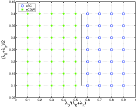
Figure 3: (Color online) Phase diagram ($u_{0}=0.0$ and $\omega_{E}=1.0$). Without on-site repulsion, the dSC phase disappears completely even for large phonon anisotropy. Color scheme is identical to Fig. (1).

As we mentioned in the introduction, the different instabilities associated with the Hubbard model at half-filling are superconductivity (sSC, dSC), antiferromagnetism (sSDW, dSDW), and charge density wave (sCDW, dCDW) with the corresponding couplingsSchulz1987 (we suppress the implicit frequency dependence for clarity)

$$u_{\textrm{(sd)SC}} = -2(g_{2}\pm g_{3}),$$ (8)

$$u_{\textrm{(sd)SDW}} = 2(g_{4}\pm g_{3}),$$ (9)

$$u_{\textrm{(sd)CDW}} = -2(2g_{1}\pm g_{3}-g_{4}),$$ (10)

where the signs are chosen so that strong fluctuations in a channel produce a positive value for the corresponding coupling, irrespective of its attractive (SC,CDW) or repulsive (SDW) nature. Since the couplings are functions of frequency and the most divergent ones are not necessarily at zero frequencyTam , only a divergent susceptibility can determine which phase has dominant fluctuations. The corresponding order parameters for the different phases are

$$\Delta^{\textrm{SC}}(\xi,\theta,\tau) \equiv \sum_{\sigma}\sigma\Psi_{\sigma,{\mathbf{k}}}(\tau)\Psi_{-\sigma,-{\mathbf{k}}}(\tau),$$ (11)

$$\Delta^{\textrm{SDW}}(\xi,\theta,\tau) \equiv \sum_{\sigma}\bar{\Psi}_{\sigma,{\mathbf{k}}}(\tau)\Psi_{-\sigma,{\mathbf{k}}+(\pi,\pi)}(\tau),$$ (12)

$$\Delta^{\textrm{CDW}}(\xi,\theta,\tau) \equiv \sum_{\sigma}\bar{\Psi}_{\sigma,{\mathbf{k}}}(\tau)\Psi_{\sigma,{\mathbf{k}}+(\pi,\pi)}(\tau),$$ (13)

and involve the creation of particle-particle (p-p) and particle-hole (p-h) pairs at given angle $\theta$ and energy $\xi$ set by ${\mathbf{k}}$. The homogeneous frequency-dependent susceptibilities associated with these order parameters are calculated by extending the one-loop RG scheme of Zanchi and SchulzZanchi2000 . Their definition involves scattering processes between pairs at different angles $\theta$ with energies corresponding to fast modes and are given by

$$\chi^{\delta}(\theta_{1},\theta_{2},|\tau_{1}-\tau_{2}|)=\prod_{i=1}^{2}\int d\xi_{i}\Theta(|\xi_{i}|-\Lambda_{\ell})J(\xi_{i},\theta_{i})$$

$$\times\langle\Delta^{\delta}(\xi_{1},\theta_{1},\tau_{1})\bar{\Delta}^{\delta}(\xi_{2},\theta_{2},\tau_{2})\rangle,$$ (14)

where $J(\xi,\theta)$ is the Jacobian for the ${\mathbf{k}}\rightarrow(\xi,\theta)$ transformation, and $\delta=$(SC,SDW,CDW). In the two-patch approximation $\theta$ can take only two values and each susceptibility becomes a $2\times 2$ matrix that we diagonalize to extract the symmetric (s-wave) and antisymmetric (d-wave) eigenvectors of each corresponding order. The interested reader is urged again to refer to the Appendix where we provide the full expressions for the susceptibility flow equations of all the different orders calculated to one-loop accuracy.

III Results

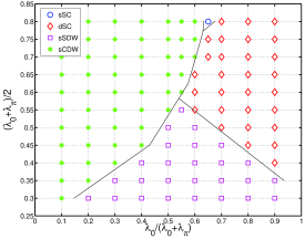
Figure 4: (Color online) Phase diagram for the same on-site repulsion ($u_{0}=0.5$) as in Fig. (1), but for a smaller phonon frequency ($\omega_{E}=0.1$). Slower phonons suppress superconductivity over the nesting-associated CDW and SDW phases. Color scheme is identical to Fig. (1).

In Fig. (2) we show the numerical solution of the RG flow equations for the couplings with $\omega_{1}=\omega_{2}=\omega_{3}=0$ (inset) and the corresponding static ($\omega=0$) homogeneous susceptibilities for the case of $\lambda_{0}=0.6$, $\lambda_{\pi}=0.4$, $\omega_{E}=1.0$, and $u_{0}=0.5$. All parameters are expressed in energy units of $2t$ (a quarter of the band width) and for the numerical implementation the frequencies are discretized into a total of $N=41$ divisions up to a maximum value of $\omega_{\rm max}=6.0$. The particular choice of $\lambda_{0}>\lambda_{\pi}$ enhances the attractive BCS type pairing processes associated with $g_{2}$, while suppressing the dominant repulsive nesting channels of $g_{3}$ (Eqs. (6-7)), and tilts the balance between the usually dominant sSDW and subdominant dSC phase. When reversed ($\lambda_{\pi}>\lambda_{0}$), the attractive channels of $g_{3}$ combined with $g_{1}$ lead to a CDW instability.

The general phase diagram for fixed values of $u_{0}=0.5$ and $\omega_{E}=1.0$ is shown in Fig. (1), where the e-ph coupling is parametrized by the mean value $\bar{\lambda}=(\lambda_{0}+\lambda_{\pi})/2$ and relative anisotropy $r=\lambda_{0}/(\lambda_{0}+\lambda_{\pi})$. Previous work on the phononic effects in this type of system was limited along $r=0.5$ (isotropic phonons) and $\bar{\lambda}\gg u_{0}$ and found the nesting-related dominant CDW competing with sSC, while dSC was suppressedBerger1995 . In our generic study, extending to all possible configurations of coupled e-ph systems, we find that close to $\bar{\lambda}=u_{0}$ and along $r=0.5$ there are four competing phases including dSC. Deep in the repulsive region antiferromagnetism prevails as expected (the counterpart of sCDW), but for $r>0.5$ type of anisotropy ($\lambda_{0}>\lambda_{\pi}$), there is a large region of dSC dominance (the case of Fig. (2) is a point in that region). Another candidate for this parameter space is dCDW (charge flux phase)dcdw but we find that while this channel does get renormalized significantly (Fig. 2), the suppressed $g_{1}$ and $g_{3}$ couplings undermine its strength.

It should be pointed out explicitly that the generic characteristics of the phase diagram in Fig. (1) are independent of the actual value of the repulsive $u_{0}$. The same phase diagram is always expected near $\bar{\lambda}=u_{0}$ and details such as adding a next-nearest neighbor hoping term in the Hamiltonian or doping away from half-filling will only $\it{enhance}$ our findings associated with dSC since all nesting-related processes will then be additionally suppressed. In the absence of Hubbard on-site repulsion ($u_{0}=0$), not only sSDW does not occur, as expected, but the dSC phase also disappears completely as shown in Fig. (3) for the $\omega_{E}=1.0$ case. Therefore, the dSC phase is not being driven solely by anisotropic phonons, but by the combined effect of anisotropic phonons, on-site repulsion and nesting of the FS.

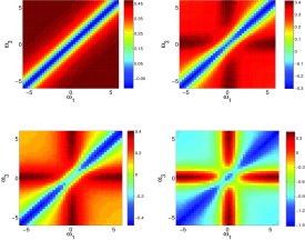
Figure 5: (Color online) Evolution of $g_{2}(\omega_{1},-\omega_{1},\omega_{3})$ coupling for $\lambda_{0}=0.6$, $\lambda_{\pi}=0.4$, and $\omega_{E}=1.0$. The RG steps chosen are $\ell=0.4,2.4,3.4,4.9$ (top left, top right, bottom left, bottom right). The color scheme is from lower dark blue (attractive) to higher dark red (repulsive) values.

In order to demonstrate the importance of retardation, we show in Fig. (4) the corresponding phase diagram for slower phonons of $\omega_{E}=0.1$, keeping $u_{0}=0.5$ fixed. We see that as compared to Fig. (1), the SC regions are suppressed and pushed towards larger values of $\bar{\lambda}$. This is a clear indication that the internal dynamics of the coupling functions extend beyond renormalizing the effective e-e interaction to attractive values. There is a rich internal frequency structure among the couplings as we show in Fig. (5), where we plot the evolution of the pairing channel of $g_{2}(\omega_{1},-\omega_{1},\omega_{3})$ for the case referring to the dSC instability of Fig. (2). At the beginning of the flow we see the attractive part of the coupling (limited around $\omega_{3}=\omega_{1}$), to be much weaker compared to the repulsive parts. As the flow progresses, and we go beyond the initial conditions of Eqs. (6-7), the repulsive parts of the coupling are suppressed in $\omega$-space and in actual values, while the attractive parts proliferate in both. Remarkably enough, when the critical point is reached we see that the same type of scattering process can become attractive or repulsive, depending on the dynamics of the electrons being scattered, with a range of strength that extends as much as three times the bare $u_{0}$. This is a strong indication that retardation effects play a crucial and dominant role in these types of systems.

IV Conclusions

In conclusion, we have presented a one-loop functional renormalization group analysis of the Hubbard model at half-filling, self-consistently including the electron-phonon interaction. We find that different values of the e-ph coupling energy and anisotropy can tune the system into different instabilities, including sSDW, sCDW, sSC, and dSC. When only the instantaneous on-site repulsion is present, sSDW is well known to dominate. In the absence of on-site repulsion, phonon mediated attraction drives the system into sCDW and sSC phases. In the presence of both interactions, depending on the competition between them, these phases appear in different parts of the phase diagram. In addition, these interactions also cooperate to generate a dSC phase. This phase therefore only emerges because of the interplay between the physics of Coulomb interactions and phonons. Retardation effects play an important role in the onset of these phases and also determine the size of the different regions in the phase diagram.

Our work is not to be considered as a complete study of the two-dimensional Hubbard model in the presence of the e-ph interaction but as a preliminary but self-consistent study that hints towards the right physics of such a system. In other words, what the functional RG study can beautifully provide to us is an unbiased study of the instabilities associated with this type of system in a self-consistent manner to the given one-loop accuracy order, which allows us the flexibility of probing an immense parameter phase space in a rather inexpensive way (numerically and analytically). The assumptions of this approach are the weak coupling regime in the electron-phonon interaction and that the largest energy scale of the system is the bandwidth. Within this approximate method we are able to draw the first charts of the rich phase space when the fermion-boson interaction is no longer neglected but self-consistently included as well.

Appendix A Coupling and self-energy flow equations

The renormalization-group flow equations for the four couplings and the self-energy are directly derived from Eqs. (4-5) when the two-patch approximation is used which maps all momenta transfers either to $(0,0)$ or $(\pi,\pi)$ converting the intrinsically non-local flow equations to local. This procedure is very well presented in the work of Zanchi and SchulzZanchi2000 for the reader interested in the full exposition of details. Here we only highlight the basic points along with presenting the final formulas for the sake of completeness.

In the two-patch approximation the whole FS is divided into two patches (each patch has its redundant mirror image). The RG flow Eqs. (4-5) involve a delta function constraining the electronic energies $\xi_{{\mathbf{k}}}$ to be “on-shell” which can be above $(+\Lambda_{\ell})$ or below $(-\Lambda_{\ell})$ the FS. This constraint induces a one-to-one correspondence between ${\mathbf{k}}$ and $(\theta,|\xi_{{\mathbf{k}}}|=\Lambda_{\ell})$ which consequently is employed to simplify the 2D-${\mathbf{k}}$ integration into an azimuthal integration over $\theta$, with the proper Jacobian $J(\theta,\xi_{{\mathbf{k}}})$ introduced. The integrand is $\theta$-independent and one can define a general operator $\hat{F}_{\nu}$ acting on any product of two coupling functions $g_{i}(\omega_{1},\omega,\omega_{3})g_{j}(\omega_{2},\omega,\omega_{4})$ according to

$$\hat{F}_{\nu} \!\![\Omega][g_{i}g_{j}](\omega_{1},\omega,\omega_{3})(\omega_{2},\omega,\omega_{4})\equiv\frac{\Lambda_{\ell}}{\pi^{3}}\int_{0}^{\pi/4}d\theta\frac{k(\theta,-\Lambda_{\ell})}{\big{|}\frac{d\xi}{dk}(\theta,-\Lambda_{\ell})\big{|}}\int_{-\infty}^{+\infty}d\omega g_{i}(\omega_{1},\omega,\omega_{3})g_{j}(\omega_{2},\omega,\omega_{4})$$ (15)

$$\times \frac{\big{(}\omega-\Sigma_{\ell}^{\prime\prime}(\omega)\big{)}\big{(}\Omega-\Sigma_{\ell}^{\prime\prime}(\Omega)\big{)}+\nu\Lambda_{\ell}^{2}}{\big{[}\big{(}\omega-\Sigma_{\ell}^{\prime\prime}(\omega)\big{)}\big{(}\Omega-\Sigma_{\ell}^{\prime\prime}(\Omega)\big{)}+\nu\Lambda_{\ell}^{2}\big{]}^{2}+\Lambda_{\ell}^{2}\big{[}\omega-\Sigma_{\ell}^{\prime\prime}(\omega)-\nu\big{(}\Omega-\Sigma_{\ell}^{\prime\prime}(\Omega)\big{)}\big{]}^{2}},$$

where $\Omega$ depends on the external frequencies and $\omega$ (which is integrated out), $\nu=\pm$ and effectively defines two types of $\hat{F}$ operators, while $\Sigma_{\ell}^{\prime\prime}$ is the imaginary part of the self-energy. The Jacobian at half-filling has the convenient property $\oint J(\theta,-\Lambda_{\ell})=\oint J(\theta,\Lambda_{\ell})$. The complete RG flow equations for the four couplings and the imaginary part of the self-energy can then be written as

$$\!\!\!\!\!\frac{\partial g_{1}}{\partial\ell}(\omega_{1},\omega_{2},\omega_{3})=\hat{F}_{+}[\omega+\omega_{1}-\omega_{3}]\bigg{(}-2[g_{3}g_{3}+g_{1}g_{1}](\omega_{1},\omega,\omega_{3})(\omega_{4},\omega,\omega_{2})+[g_{3}g_{3}+g_{1}g_{4}](\omega_{1},\omega,\omega_{3})(\omega,\omega_{4},\omega_{2})$$ (16)

$$+ [g_{3}g_{3}+g_{4}g_{1}](\omega,\omega_{1},\omega_{3})(\omega_{4},\omega,\omega_{2})\bigg{)}+\hat{F}_{+}[\omega+\omega_{3}-\omega_{1}]\bigg{(}-2[g_{3}g_{3}+g_{1}g_{1}](\omega_{3},\omega,\omega_{1})(\omega_{2},\omega,\omega_{4})$$

$$+ [g_{3}g_{3}+g_{1}g_{4}](\omega_{3},\omega,\omega_{1})(\omega,\omega_{2},\omega_{4})+[g_{3}g_{3}+g_{4}g_{1}](\omega,\omega_{3},\omega_{1})(\omega_{2},\omega,\omega_{4})\bigg{)},$$

$$\!\!\!\!\!\frac{\partial g_{2}}{\partial\ell}(\omega_{1},\omega_{2},\omega_{3})=\hat{F}_{-}[\omega_{1}+\omega_{2}-\omega]\bigg{(}[g_{3}g_{3}+g_{2}g_{2}](\omega_{1},\omega_{2},\omega)(\omega_{3},\omega_{4},\omega)+[g_{3}g_{3}+g_{2}g_{2}](\omega_{2},\omega_{1},\omega)(\omega_{4},\omega_{3},\omega)\bigg{)}$$ (17)

$$\!\!\!\!\!\frac{\partial g_{3}}{\partial\ell}(\omega_{1},\omega_{2},\omega_{3})=\hat{F}_{+}[\omega+\omega_{1}-\omega_{3}]\bigg{(}-2[g_{3}g_{1}+g_{1}g_{3}](\omega_{1},\omega,\omega_{3})(\omega_{4},\omega,\omega_{2})+[g_{3}g_{4}+g_{1}g_{3}](\omega_{1},\omega,\omega_{3})(\omega,\omega_{4},\omega_{2})$$ (18)

$$+ [g_{3}g_{1}+g_{4}g_{3}](\omega,\omega_{1},\omega_{3})(\omega_{4},\omega,\omega_{2})\bigg{)}+\hat{F}_{+}[\omega+\omega_{3}-\omega_{1}]\bigg{(}-2[g_{3}g_{1}+g_{1}g_{3}](\omega_{3},\omega,\omega_{1})(\omega_{2},\omega,\omega_{4})$$

$$+ [g_{3}g_{4}+g_{1}g_{3}](\omega_{3},\omega,\omega_{1})(\omega,\omega_{2},\omega_{4})+[g_{3}g_{1}+g_{4}g_{3}](\omega,\omega_{3},\omega_{1})(\omega_{2},\omega,\omega_{4})\bigg{)}$$

$$+ \hat{F}_{-}[\omega_{1}+\omega_{2}-\omega]\bigg{(}[g_{2}g_{3}+g_{3}g_{2}](\omega_{1},\omega_{2},\omega)(\omega_{3},\omega_{4},\omega)+[g_{2}g_{3}+g_{3}g_{2}](\omega_{2},\omega_{1},\omega)(\omega_{4},\omega_{3},\omega)\bigg{)}$$

$$+ \hat{F}_{+}[\omega+\omega_{2}-\omega_{3}][g_{3}g_{4}+g_{4}g_{3}](\omega,\omega_{2},\omega_{3})(\omega,\omega_{4},\omega_{1})+\hat{F}_{+}[\omega+\omega_{3}-\omega_{2}][g_{3}g_{4}+g_{4}g_{3}](\omega,\omega_{3},\omega_{2})(\omega,\omega_{1},\omega_{4}),$$

$$\!\!\!\!\!\frac{\partial g_{4}}{\partial\ell}(\omega_{1},\omega_{2},\omega_{3})=\hat{F}_{+}[\omega+\omega_{2}-\omega_{3}][g_{3}g_{3}+g_{4}g_{4}](\omega,\omega_{2},\omega_{3})(\omega,\omega_{4},\omega_{1})$$ (19)

$$+ \hat{F}_{+}[\omega+\omega_{3}-\omega_{2}][g_{3}g_{3}+g_{4}g_{4}](\omega,\omega_{3},\omega_{2})(\omega,\omega_{1},\omega_{4}),$$

$$\frac{\partial\Sigma_{\ell}^{\prime\prime}}{\partial\ell}(\omega_{1}) = \frac{\Lambda_{\ell}}{\pi^{3}}\int_{0}^{\pi/4}d\theta\frac{k(\theta,-\Lambda_{\ell})}{\big{|}\frac{d\xi}{dk}(\theta,-\Lambda_{\ell})\big{|}}\int_{-\infty}^{+\infty}d\omega\frac{\big{(}[g_{1}+g_{2}](\omega_{1},\omega,\omega)-2[g_{2}+g_{4}](\omega_{1},\omega,\omega_{1})\big{)}\big{(}\omega-\Sigma_{\ell}^{\prime\prime}(\omega)\big{)}}{\big{(}\omega-\Sigma_{\ell}^{\prime\prime}(\omega)\big{)}^{2}+\Lambda_{\ell}^{2}}.$$ (20)

The above equations are numerically solved for each RG step $\ell$ until any coupling for any frequency channel diverges to values greater than $20t$ at which point we stop the algorithm and form all the couplings associated with the different instabilities given by Eqs (8-10). For frequency independent interactions the above equations reduce to the usualSchulz1987

$$\frac{\partial g_{1}}{\partial\ell} = -2g_{1}(g_{1}-g_{4}),$$ (21)

$$\frac{\partial g_{2}}{\partial\ell} = -g_{2}^{2}-g_{3}^{2},$$ (22)

$$\frac{\partial g_{3}}{\partial\ell} = -2g_{3}(g_{1}+g_{2}-2g_{4}),$$ (23)

$$\frac{\partial g_{4}}{\partial\ell} = g_{3}^{2}+g_{4}^{2}.$$ (24)

Appendix B Susceptibility flow equations

Once the RG flow for the couplings is numerically solved and the divergence point towards strong coupling is reached we calculate the susceptibilities associated with the major orders in the system. As we mentioned in the text, a general susceptibility calculation involves Eq. (14) for all different orders. By including (to one-loop) all RG vertex correctionsZanchi2000 we obtain the general homogeneous susceptibility flow equation which in the two-patch approximation reduces to a $2\times 2$ matrix given by

$$\!\!\!\!\!\!\partial_{\ell}\chi^{\delta}_{\ell}\!(\omega_{1})\!=\!\frac{\Lambda_{\ell}}{\pi^{3}}\!\!\int_{0}^{\pi/4}\!\!\!\!d\theta J(\theta,-\Lambda_{\ell})\!\!\int_{-\infty}^{+\infty}\!\!\!\!d\omega W_{\ell}^{\delta}(\omega_{1},\omega)$$ (25)

$$\times \begin{pmatrix}z_{11}z_{11}+z_{12}z_{21}&z_{11}z_{12}+z_{12}z_{22}\\ z_{21}z_{11}+z_{22}z_{21}&z_{22}z_{22}+z_{21}z_{12}\end{pmatrix},$$

where $\delta=(AF,SC,CDW)$ and we have used the shorthand notation $z_{ij}z_{lm}=z^{\delta}(\theta_{i},\theta_{j};\omega_{1},\omega)z^{\delta}(\theta_{l},\theta_{m};\omega,\omega_{1})$ and the definitions

$$\!\!\!\!\!\!\!\!W_{\ell}^{AF}(\omega_{1},\omega)=W_{\ell}^{CDW}(\omega_{1},\omega)=$$

$$\!\!\!\!\!\!\!\!\frac{\Lambda_{\ell}^{2}\!+\!\big{(}\omega\!-\!\Sigma^{\prime\prime}_{\ell}(\omega)\big{)}\big{(}\omega\!+\!\omega_{1}\!-\!\Sigma^{\prime\prime}_{\ell}(\omega\!+\!\omega_{1})\big{)}}{\big{[}\big{(}\omega\!-\!\Sigma^{\prime\prime}(\omega)\big{)}^{2}\!\!\!+\!\!\Lambda_{\ell}^{2}\big{]}\big{[}\big{(}\omega\!+\!\omega_{1}\!-\!\Sigma^{\prime\prime}_{\ell}(\omega\!+\!\omega_{1})\big{)}^{2}\!\!\!+\!\!\Lambda_{\ell}^{2}\big{]}},$$ (26)

$$\!\!\!\!\!\!\!\!W_{\ell}^{SC}(\omega_{1},\omega)=$$

$$\!\!\!\!\!\!\!\!\frac{\Lambda_{\ell}^{2}\!-\!\big{(}\omega\!-\!\Sigma^{\prime\prime}_{\ell}(\omega)\big{)}\big{(}\omega_{1}\!-\!\omega\!-\!\Sigma^{\prime\prime}_{\ell}(\omega_{1}\!-\!\omega)\big{)}}{\big{[}\big{(}\omega\!-\!\Sigma^{\prime\prime}(\omega)\big{)}^{2}\!\!\!+\!\!\Lambda_{\ell}^{2}\big{]}\big{[}\big{(}\omega_{1}\!-\!\omega\!-\!\Sigma^{\prime\prime}_{\ell}(\omega_{1}\!\!-\!\omega)\big{)}^{2}\!\!\!+\!\!\Lambda_{\ell}^{2}\big{]}}.$$ (27)

The RG flow equations for the vertex functions associated with the nested related phases are given by

$$\!\!\!\!\!\partial_{\ell}z^{AF}_{\ell}\!\!(\omega_{1},\omega_{2})\!=\!\frac{\Lambda_{\ell}}{\pi^{3}}\!\!\int_{0}^{\pi/4}\!\!\!\!d\theta J(\theta,-\Lambda_{\ell})\!\!\int_{-\infty}^{+\infty}\!\!\!\!d\omega W_{\ell}^{AF}(\omega_{1},\omega)$$

$$\times\begin{pmatrix}z_{11}g_{3}+z_{12}g_{4}&z_{11}g_{4}+z_{12}g_{3}\\ z_{21}g_{3}+z_{22}g_{4}&z_{21}g_{4}+z_{22}g_{3}\end{pmatrix},$$ (28)

and

$$\!\!\!\!\!\!\!\partial_{\ell}z^{CDW}_{\ell}\!\!(\omega_{1},\omega_{2})\!\!=\!\!\frac{-\Lambda_{\ell}}{\pi^{3}}\!\!\!\int_{0}^{\pi/4}\!\!\!\!\!\!\!\!d\theta J(\theta,-\Lambda_{\ell})\!\!\!\int_{-\infty}^{+\infty}\!\!\!\!\!\!\!\!d\omega W_{\ell}^{CDW}\!\!(\omega_{1},\omega)$$

$$\times\begin{pmatrix}z_{11}g_{\alpha}+z_{12}g_{\beta}&z_{11}g_{\beta}+z_{12}g_{\alpha}\\ z_{21}g_{\alpha}+z_{22}g_{\beta}&z_{21}g_{\beta}+z_{22}g_{\alpha}\end{pmatrix},$$ (29)

where $z_{ij}g_{k}\equiv z^{\delta}(\theta_{i},\theta_{j};\omega_{1},\omega)g_{k}(\omega_{2},\omega_{1}+\omega,\omega)$ and we used the additional definitions

$$\!\!\!\!\!\!\!\!\!g_{\alpha}\!(\omega_{2},\omega_{1}\!\!+\!\!\omega,\omega)\!\!\! \equiv \!\!\!2g_{3}(\omega_{1}\!\!+\!\!\omega,\omega_{2},\omega)\!\!-\!\!g_{3}(\omega_{2},\omega_{1}\!\!+\!\!\omega,\omega),$$ (30)

$$\!\!\!\!\!\!\!\!\!g_{\beta}\!(\omega_{2},\omega_{1}\!\!+\!\!\omega,\omega)\!\!\! \equiv \!\!\!2g_{1}(\omega_{1}\!\!+\!\!\omega,\omega_{2},\omega)\!\!-\!\!g_{4}(\omega_{2},\omega_{1}\!\!+\!\!\omega,\omega).$$ (31)

For the SC-related vertex function we have

$$\!\!\!\!\!\partial_{\ell}z^{SC}_{\ell}\!(\omega_{1},\omega_{2})\!=\!\frac{\Lambda_{\ell}}{\pi^{3}}\!\!\int_{0}^{\pi/4}\!\!\!\!\!d\theta J(\theta,-\Lambda_{\ell})\!\!\int_{-\infty}^{+\infty}\!\!\!\!\!d\omega W_{\ell}^{SC}(\omega_{1},\omega)$$

$$\times\begin{pmatrix}z_{11}g_{2}+z_{12}g_{3}&z_{11}g_{3}+z_{12}g_{2}\\ z_{21}g_{2}+z_{22}g_{3}&z_{21}g_{3}+z_{22}g_{2}\end{pmatrix}.$$ (32)

where $z_{ij}g_{k}\equiv z^{SC}(\theta_{i},\theta_{j};\omega_{1},\omega)g_{k}(\omega,\omega_{1}-\omega,\omega_{2})$. All susceptibilities are zero at the initial RG step $\ell=0$, and the vertex functions obey

$$z^{\delta}_{\ell=0}(\theta_{1},\theta_{2};\omega_{1},\omega_{2})=\frac{1}{4}\delta_{\theta_{1},\theta_{2}}\delta(\omega_{1}-\omega_{2}).$$ (33)

Also, due to the fact that we are at half-filling the flow equations for the nested related phases are localZanchi2000 .

References

• (1) S.-W. Tsai, A. H. Castro Neto, R. Shankar, and D. K Campbell, Phys. Rev. B 72, 054531 (2005).
• (2) R. Shankar, Rev. Mod. Phys. 66, 129 (1994).
• (3) E. Faulques, V. G. Ivanov, C. Mézière, and P. Batail, Phys. Rev. B 62, R9291 (2000), L. Pintschovious, H. Rietschel, T. Sasaki, H. Mori, S. Tanaka, N. Toyota, M. Lang, and F. Steglich, Europhys. Lett. 37, 627 (1997).
• (4) A. Lanzara, P. V. Bogdanov, X. J. Zhou, S. A. Kellar, D. L. Feng, E. D. Lu, T. Yoshida, H. Eisaki, A. Fujimori, K. Kishio, J.-I. Shimoyama, T. Noda, S. Uchida, Z. Hussain, and Z.-X. Shen, Nature 412, 510 (2001); X. J. Zhou, T. Cuk, T. Devereaux, N. Nagaosa, Z.-X. Shen, cond-mat/0604284.
• (5) A. P. Litvinchuk, C. Thomsen, and M. Cardona, in “Physical Properties of High Temperature Superconductors” IV, edited by D. M. Ginsberg (World Scientific, Singapore, 1994), p. 375, and references therein.
• (6) S. Lupi, M. Ortolani, L. Baldassarre, P. Calvani, D.Prabhakaran, and A. T. Boothroyd, cond-mat/0501746
• (7) “Conjugated Conducting Polymers”, edited by H. G. Weiss (Springer-Verlag, Berlin, 1992).
• (8) L. Mathey, S.-W. Tsai, and A. H. Castro Neto, Phys. Rev. Lett. 97, 030601 (2006)
• (9) H. J. Schulz, Europhys. Lett. 4, 609 (1987).
• (10) P. Lederer, G. Montambaux, and D. Poilblanc, J. Phys. 48, 1613 (1987); J. González, F. Guinea and M. A. H. Vozmediano, Phys. Rev. Lett. 79, 3514 (1997); ibid., 84, 4930 (2000); N. Furukawa, T. M. Rice, and M. Salmhofer, Phys. Rev. Lett. 81, 3195 (1998); C. Honerkamp, M. Salmhofer, N. Furukawa, and T. Rice. Phys. Rev. B 63, 035109 (2001); B. Binz, D. Baeriswyl and B. Douçot, Eur. Phys. J. B 25, 69 (2002); A. A. Katanin and A. P. Kampf, Phys. Rev. B 68, 195101 (2003); G. Aprea, C. Di Castro, M. Grilli, and J. Lorenzana, cond-mat/0601374
• (11) J. González, F. Guinea and M. A. H. Vozmediano, Europhys. Lett. 34, 711 (1996).
• (12) David Sénéchal, P.-L. Lavertu, M.-A. Marois, and A.-M. S. Tremblay, Phys. Rev. Lett. 94, 156404 (2005)
• (13) E. Berger, P. Valášek, and W. von der Linden, Phys. Rev. B 52, 4806 (1995).
• (14) J. M. Williams, M. Jack, Arthur J. Schultz, Urs Geiser, K. D. Carlson, Aravinda M. Kini, Science 252, 1501 (1991); D. Jerome, Science 252, 1509 (1991).
• (15) J. Polchinski, Nucl. Phys. B 231, 269 (1984)
• (16) D. Zanchi and H. J. Schulz, Phys. Rev. B 61, 13609 (2000)
• (17) C. Halboth and W. Metzner, Phys. Rev. B 61, 7364 (2000)
• (18) B. Binz, D. Baeriswyl, and B. Douçot, Ann. Phys. (Leipzig) 12, 704 (2003).
• (19) J. González, Phys. Rev. B 63, 045114 (2001); R. Roldán, M. P. López-Sancho, F. Guinea, and S.-W. Tsai, cond-mat/0603673.
• (20) I. Affleck, and J. B. Marston, Phys. Rev. B 37, 3774 (1988); S. Chakravarty, R. B. Laughlin, D. K. Morr, and C. Nayak, Phys. Rev. B 63, 094503 (2001)
• (21) K.-M. Tam, S.-W. Tsai, D. K. Campbell, and A. H. Castro Neto, unpublished.