Double exchange model for correlated electrons in systems with $t_{2g}$ orbital degeneracy

Abstract

We formulate the double exchange (DE) model for systems with $t_{2g}$ orbital degeneracy, relevant for hole-doped cubic vanadates. In the relevant regime of strong on-site Coulomb repulsion $U$ we solve the model using two distinct mean-field approximations: Hartree-Fock, and mean-field applied to the formulation of the model in the Kotliar-Ruckenstein slave boson represenation. We show how, due to the relative weakness of the DE mechanism via $t_{2g}$ degenerate orbitals, the anisotropic $C$-type antiferromagnetic metallic phase and the orbital liquid state can be stabilized. This is contrasted with the DE mechanism via $e_{g}$ degenerate orbitals which stabilizes the ferromagnetic order in the hole-doped regime of manganites. The obtained results are in striking agreement with the observed magnetic structures and the collapse of the orbital order in the doped La_1-xSr_xVO₃, Pr_1-xCa_xVO₃ and Nd_1-xSr_xVO₃.

1 Introduction

Recently orbital degrees of freedom in the strongly correlated electron systems have attracted much attention [1] due to their crucial role in the stability of the various magnetic phases in the Mott insulators [2] or in the partial explanation of the Mott metal-insulator transition itself [3]. Typical examples of such systems are the transition-metal oxides with partly filled $e_{g}$ or $t_{2g}$ degenerate orbitals. The remarkable feature of these oxides is the large on-site Coulomb repulsion $U\gg t$, with $t$ being the effective electron hopping. In case of the stoichiometric (undoped) oxides the Coulomb repulsion between electrons supresses charge fluctuations and leads to the effective low-energy $\propto\!J\!\!=\!\!4t^{2}\!/U$ superexchange (SE) interactions between spin and orbital degrees of freedom. In addition, the atomic Hund’s interaction $J_{H}\ll U$ aligns the spins of the electrons occupying the degenerate and almost degenerate orbitals on the same site and should be taken into account in the realistic SE-type models. Interestingly, it is the Hund’s interaction which to large extent stabilizes particular spin (magnetic) and orbital order. It should be stressed that though the $e_{g}$ orbitals usually order as in e.g. LaMnO₃ [2], it is rather not the case of the $t_{2g}$ orbitals which can form a disordered quantum orbital liquid (OL) as in e.g. LaVO₃ [4]. The different kinds of the orbital state are concomitant with various anisotropic magnetic phases such as $A$-AF [ferromagnetic (FM) planes staggered antiferromagnetically (AF) in the other direction] in LaMnO₃ [2] or $C$-AF [FM chains staggered AF in the other two directions] in LaVO₃ [4].

Doping with holes destroys the insulating state, modifies the SE interaction and hence can also modify the magnetic order and orbital state stabilized in the undoped case. In such systems the motion of holes is strongly affected by: (i) intersite SE interaction $\propto J$, (ii) on-site Hund’s interaction $\propto J_{H}$, which is captured by the Kondo-lattice model. In the realistic limit in the transition metal oxides $J_{H}\gg t\gg J$ this model reduces to the double exchange model (DE) [5]. However, for the above discussed class of the transition-metal oxides, orbital degeneracy needs also to be taken into account in such a model. This was done in the seminal work of van den Brink and Khomskii [6] for electrons with the $e_{g}$ degeneracy, leading to a naively counterintuitive picture of the DE mechanism. One can thus pose a question how the DE mechanism would be modified in the case of the $t_{2g}$ orbital degeneracy, as the SE interactions for the undoped oxides differ qualitatively for the $t_{2g}$ and $e_{g}$ cases. Hence, in this paper we want to answer three questions: (i) what is the nature of the magnetic order stabilized by the DE mechanism for correlated electrons with $t_{2g}$ orbital degeneracy, (ii) what is the nature of the orbital order, and (iii) how do these results differ from the $e_{g}$ and the nondegenerate case.

The paper is organized as follows. In the following chapter we introduce the DE Hamiltonian with $t_{2g}$ orbital degrees of freedom. Then we solve the model using two different mean-field approximations and we show that the metallic state coexists with the $C$-AF order and OL state for the broad range of hole-doping. Next we discuss the results, i.e.: the validity of the approximations, the generic role of the $t_{2g}$ orbitals in the stability of the above phases, the physical relevance of the model by comparison with the experiment. The paper is concluded by stressing: the distinct features of the DE mechanism via $e_{g}$ and via $t_{2g}$ degenerate orbitals, and the crucial role of the Coulomb repulsion $U$.

2 Realistic double exchange Hamiltonian

We start with the realistic semiclassical DE Hamiltonian with $t_{2g}$ orbital degrees of freedom, relevant for the hole-doped cubic vanadates [7]:

$${\cal H}_{\rm DE}=-u_{y}\sum_{i,j\|\hat{y}}\widetilde{a}^{\dagger}_{i}\widetilde{a}_{j}\ -\sum_{i,j\|\hat{z}}\widetilde{a}_{i}^{\dagger}\widetilde{a}_{j}\ -u_{x}\sum_{i,j\|\hat{x}}\widetilde{b}^{\dagger}_{i}\widetilde{b}_{j}\ -\sum_{i,j\|\hat{z}}\widetilde{b}_{i}^{\dagger}\widetilde{b}_{j}\ +J\!\!\sum_{\langle ij\rangle\|\hat{x},\hat{y}}\!\text{\bf{S}}_{i}\cdot\text{\bf{S}}_{j}.$$ (1)

where: the hopping amplitude $t\!\!=\!\!1$; the restricted fermion creation operators ${\widetilde{a}}^{\dagger}_{i}=a^{\dagger}_{i}(1-b_{i}^{\dagger}b_{i})$, ${\widetilde{b}}^{\dagger}_{i}=b^{\dagger}_{i}(1-a_{i}^{\dagger}a_{i})$, where $a^{\dagger}_{i}(b^{\dagger}_{i})$ creates a spinless electron at site $i$ in $yz(zx)$ orbital; and $\text{\bf{S}}_{i}$ are core spin $S=1/2$ operators of $t_{2g}$ electrons in occupied $xy$ orbitals. We introduce the $u_{x}$ and $u_{y}$ variational parameters to be defined later. The Hamiltonian has the following features: (i) the first four terms describe the kinetic energy of the electrons in the degenerate $yz$ and $zx$ orbitals which can hop only in the allowed $(\hat{y},\hat{z})$ or $(\hat{x},\hat{z})$ plane to the nearest neighbour (nn) site $i$ providing there are no other electrons at site $i$ in these orbitals ($U=\infty$ assumed implicitly), (ii) the last term describes the AF coupling between core spins at nn sites in the $(\hat{x},\hat{y})$ plane due to the SE interaction originating from the electrons in the always occupied $xy$ orbitals ($n_{xy}=1$ during doping), (iii) the SE interactions due to the itinerant electrons in $yz$ and $zx$ orbitals are neglected.

The variational parameters are defined as $u_{x}=\cos(\theta_{x}/2)$ and $u_{y}=\cos(\theta_{y}/2)$, where $\theta_{x}$ $(\theta_{y})$ is the relative angle between core spins in the $\hat{x}$ $(\hat{y})$ direction. This follows from the Hund’s rule which aligns the spins of the itinerant electrons with the core spins and which is not explicitly written in Eq. (1) but enters via $u_{x}$ and $u_{y}$ parameters. Then the last term of Eq. (1) can be written as:

$${E}_{\rm SE}=J\!\sum_{\langle ij\rangle\|\hat{x},\hat{y}}\!\text{\bf{S}}_{i}\cdot\text{\bf{S}}_{j}=\frac{J}{2}L^{3}(u_{x}^{2}\!+\!u_{y}^{2}\!-\!1),$$ (2)

where $L^{3}$ is the number of sites in the crystal. Eq.(1) together with Eq. (2) shows the competition between the DE mechanism allowing for the hopping in the underlying FM background with the SE interaction supporting the AF order.

3 Numerical results

The ground state of Eq. (1) was found using two distinct mean-field approximations: Hartree-Fock, and mean-field applied to the formulation of the model Eq. (1) in the Kotliar-Ruckenstein slave boson representation [8].

3.1 Hartree-Fock approximation (HFA)

To facilitate the treatment of the hole doped electronic systems we enlarge the original Fock space, which is relevant for the Hamiltonian Eq. (1), by adding a boson creation (annhilation) operator $e^{\dagger}_{i}(e_{i})$, which creates (annihilates) a charged hole. Then, in order to get rid of the nonphysical states in the enlarged Fock space we need a local constraint:

$$\forall_{i}\quad a^{\dagger}_{i}a_{i}+b_{i}^{\dagger}b_{i}+e_{i}^{\dagger}e_{i}=1.$$ (3)

Note that the boson controlling double occupancies is not introduced since such configurations are forbidden for $U=\infty$. In order to solve Eq. (1) with the constraint Eq. (3) in a simple way, we introduce mean-field approximation for the above constraint and replace the following combination of fermion operators by averages:

$$\forall_{i}\quad b^{\dagger}_{i}b_{i}\rightarrow\langle b^{\dagger}_{i}b_{i}\rangle=:\delta\ \text{and}\ 0\leq\delta\leq 1,$$ (4)

$$\forall_{i}\quad a^{\dagger}_{i}a_{i}\rightarrow\langle a^{\dagger}_{i}a_{i}\rangle=1-x-\delta\ \text{and}\ 0\leq\delta+x\leq 1,$$ (5)

where in Eq. (5) we use constraint Eq. (3), where $\langle e^{\dagger}_{i}e_{i}\rangle=x$ and $x$ is the number of doped holes per site. Besides, the inequalities in Eq. (4) and (5) follow from the fact that we are discussing the hole-doping regime, i.e. with not more than one itinerant electron per site. We call this mean-field approximation an HFA approximation since it is equivalent to decoupling the interaction term in an HFA way:

$$(U\!-\!3J_{H})\ a^{\dagger}_{i}a_{i}b^{\dagger}_{i}b_{i}\simeq(U\!-\!3J_{H})\left(\langle a^{\dagger}_{i}a_{i}\rangle b^{\dagger}_{i}b_{i}\!+\!a^{\dagger}_{i}a_{i}\langle b^{\dagger}_{i}b_{i}\rangle\!-\!\langle a_{i}a^{\dagger}_{i}\rangle\langle b^{\dagger}_{i}b_{i}\rangle\right),$$ (6)

and then making the $U\rightarrow\infty$ limit [where $U-3J_{H}$ is the energy of the $t_{2g}^{2}$ high spin state]. Note that the above used HFA does not allow for the alternating orbital (AO) order but we do not expect such an order to persist during doping. This is because the kinetic energy of the electrons in the AO is rigorously zero for $U=\infty$ and the vanishing hopping between different orbitals [9].

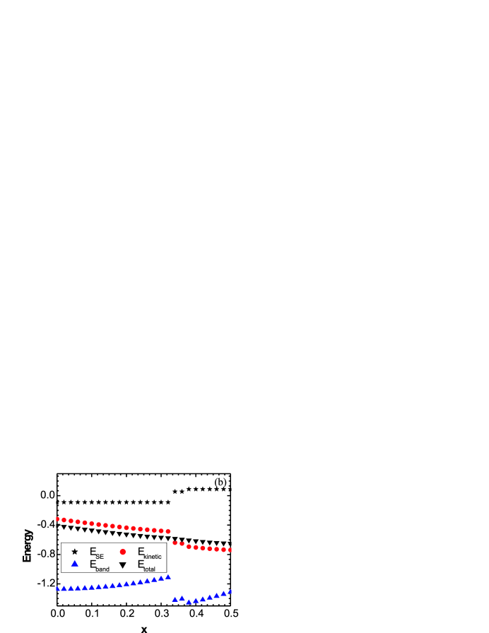
Figure 1: Results of the minimisation of Eq. (7) (with the constraint Eq. (9)): (a) Magnetic phase diagram at $T=0$. Under increasing hole doping $x$, the $C$-AF order changes via the canted Ca** phase, with spins canted on two bonds, to a homogenous FM phase. The grey horizontal line depicts the realistic value of SE $J=0.18$ in LaVO₃; (b) Competing: correlated kinetic energy ($E_{\rm kinetic}$), and magnetic energy ($E_{\rm SE}$) as a function of hole doping $x$ for the fixed value of SE $J=0.18$. Kinetic energy for uncorrelated electrons ($E_{\rm band}$) and the total energy of the system ($E_{\rm total}$) is also shown.

Then $\mathcal{H}_{\rm DE}$ can be diagonalized and the total energy of the system in the mean-field approximation is:

$$E_{\rm HFA}/L\!=\!(\!1\!\!-\!\!\delta)^{2}\!\sum_{\begin{subarray}{c}(k_{y},k_{z})\in\\ S_{F}(u_{y},1\!-\!x\!-\!\delta)\end{subarray}}\!\!\!\mathcal{E}(k_{y},k_{z};u_{y})\!+\!(\!x\!\!+\!\!\delta)^{2}\!\sum_{\begin{subarray}{c}(k_{x},k_{z})\in\\ S_{F}(u_{x},\delta)\end{subarray}}\mathcal{E}(k_{x},k_{z};u_{x})+E_{\rm SE}$$ (7)

where the kinetic energy renormalizing factors follow from the HFA. The sums go over the mesh of $\bf{k}$’s belonging to the Fermi volume $S_{F}$ which "accommodates" $1-x-\delta$ or $\delta$ electrons per site (respectively) and whose shape depends also on the band dispersion relations for the tight-binding model renormalized by the underlying magnetic order:

$$\mathcal{E}(k_{y},k_{z};u_{y})\!=\!-2(u_{y}\cos k_{y}\!+\!\cos k_{z})\ {\rm and}\ \mathcal{E}(k_{x},k_{z};u_{x})\!=\!-2(u_{x}\cos k_{x}\!+\!\cos k_{z}).$$ (8)

Since we are calculating separately the energies of the $yz$ and $zx$ bands we need an additional constraint for the Fermi levels $\mathcal{E}_{F}$ as the two bands fill up gradually:

$$\mathcal{E}_{F}(1-x-\delta,u_{y})=\mathcal{E}_{F}(\delta,u_{x}).$$ (9)

For fixed values of SE $J$ and hole doping $x$ we minimise numerically the total energy Eq. (7) (with the constraint Eq. (9)) with respect to the $u_{x}$ and $u_{y}$ variational parameters, which determine the magnetic structure. The resulting magnetic phase diagram at $T=0$ is shown in Fig. 1(a). In Fig. 1(b) we show the competing kinetic and magnetic (SE) energies as a function of hole doping $x$ for the realistic value of SE $J=0.18$ and obtained in the minimum of the total energy. Let us also note that for all of the discussed values of $J$ and $x$ it was found that $\delta^{min}=\langle c^{\dagger}_{i}c_{i}\rangle=\langle d^{\dagger}_{i}d_{i}\rangle=(1-x)/2$, i.e. the number of electrons in both orbitals is the same and the ferrorbital order (FO) is not stabilized.

3.2 Kotliar-Rukenstein slave boson approach (KRA)

We rewrite the Hamiltonian Eq. (1) using Kotliar-Ruckenstein slave boson representation [8] adopted to the orbital case. So we enlarge the Fock space by introducing three auxiliary boson fields and decouple the electron creation operator $a^{\dagger}_{i}(b^{\dagger}_{i})$ into a fermion creation operator $f^{\dagger}_{i}(g^{\dagger}_{i})$ carrying the orbital degree of freedom (orbital flavour), a boson creation operator $p^{\dagger}_{i}(q^{\dagger}_{i})$, and a boson annihilation operator $e_{i}$ carrying the charge degree of freedom (i.e. $e^{\dagger}_{i}$ creates a charged hole):

$$a^{\dagger}_{i}=f^{\dagger}_{i}z^{\dagger}_{i},\quad b^{\dagger}_{i}=g^{\dagger}_{i}y^{\dagger}_{i},$$ (10)

where

$$z^{\dagger}_{i}\!:=\!\frac{p^{\dagger}_{i}e_{i}}{\sqrt{(1-e^{\dagger}e_{i}\!-\!q_{i}^{\dagger}q_{i})(1\!-\!p_{i}^{\dagger}p_{i})}},\ \ {\rm and}\ \ y^{\dagger}_{i}\!:=\!\frac{q^{\dagger}_{i}e_{i}}{\sqrt{(1-e^{\dagger}e_{i}\!-\!p_{i}^{\dagger}p_{i})(1\!-\!q_{i}^{\dagger}q_{i})}}.$$ (11)

Applying this to the Hamiltonian $\mathcal{H}_{\rm DE}$ we get:

$$\mathcal{H}_{\rm DE}= -u_{y}\sum_{i,j\|\hat{y}}{f}^{\dagger}_{i}{f}_{j}z^{\dagger}_{i}z_{j}-\sum_{i,j\|\hat{z}}{f}^{\dagger}_{i}{f}_{j}z^{\dagger}_{i}z_{j}+E_{\rm SE}$$

$$-u_{x}\sum_{i,j\|\hat{x}}{g}^{\dagger}_{i}{g}_{j}y_{i}^{\dagger}y_{j}-\sum_{i,j\|\hat{z}}{g}_{i}^{\dagger}{g}_{j}y_{i}^{\dagger}y_{j},$$ (12)

where we also need constraints to get rid of the nonphysical states in the enlarged Fock space:

$$\forall_{i}\quad p^{\dagger}_{i}p_{i}+ q_{i}^{\dagger}q_{i}+e_{i}^{\dagger}e_{i}=1,\quad\forall_{i}\quad p^{\dagger}_{i}p_{i}=f_{i}^{\dagger}f_{i}\quad\text{and}\quad\forall_{i}\quad q_{i}^{\dagger}q_{i}=g_{i}^{\dagger}g_{i}.$$ (13)

Next we introduce mean-field approximation:

$$\forall_{i}\quad z_{i}^{\dagger}z_{i}\rightarrow\langle z_{i}^{\dagger}z_{i}\rangle=\frac{\langle p^{\dagger}_{i}e_{i}e_{i}^{\dagger}p_{i}\rangle}{\langle 1-e^{\dagger}e_{i}-q_{i}^{\dagger}q_{i}\rangle\langle 1-p_{i}^{\dagger}p_{i}\rangle}=\frac{x}{x_{a}},$$

$$\forall_{i}\quad y_{i}^{\dagger}y_{i}\rightarrow\langle y_{i}^{\dagger}y_{i}\rangle=\frac{\langle q^{\dagger}_{i}e_{i}e_{i}^{\dagger}q_{i}\rangle}{\langle 1-e^{\dagger}e_{i}-p_{i}^{\dagger}p_{i}\rangle\langle 1-q_{i}^{\dagger}q_{i}\rangle}=\frac{x}{x_{b}},$$ (14)

where we use Eq. (13) and introduce: $\langle 1-p_{i}^{\dagger}p_{i}\rangle=x_{a}$ the mean number of holes per site in orbital $yz$, $\langle 1-q_{i}^{\dagger}q_{i}\rangle=x_{b}$ the mean number of holes per site in orbital $zx$, and $\langle e^{\dagger}_{i}e_{i}\rangle=x$ the mean number of holes per site. Furthermore, introducing parameter $\delta$ defined in the same manner as in Eq. (4-5) yields $x_{a}=x+\delta$ and $x_{b}=1-\delta$. Then the total energy of the system in the mean-field approximation is:

$$E_{\rm KRA}/L=\ \frac{x}{x+\delta}\!\!\!\sum_{\begin{subarray}{c}(k_{y},k_{z})\in\\ S_{F}(u_{y},1-x-\delta)\end{subarray}}\!\!\!\mathcal{E}(k_{y},k_{z};u_{y})+\frac{x}{1-\delta}\!\!\!\sum_{\begin{subarray}{c}(k_{x},k_{z})\in\\ S_{F}(u_{x},\delta)\end{subarray}}\!\mathcal{E}(k_{x},k_{z};u_{x})+E_{\rm SE},$$ (15)

where the electronic bands are defined in the same manner as in Eq. (8) and the constraint Eq. (9) also holds.

As in the HFA we deduce the resulting magnetic structures by minimising the total energy Eq. (15) with the constraint Eq. (9). The resulting magnetic phases are shown in Fig. 2(a) and the competing energies at fixed SE $J$ as a function of hole doping $x$ are shown in Fig. 2(b). We should also stress that the number of electrons in both orbitals does not change during doping and is equal to $\delta^{min}=(1-x)/2$. Hence, the kinetic energy renormalizing factors are equal to $2x/(x+1)$, the well-known Gutzwiller factors.

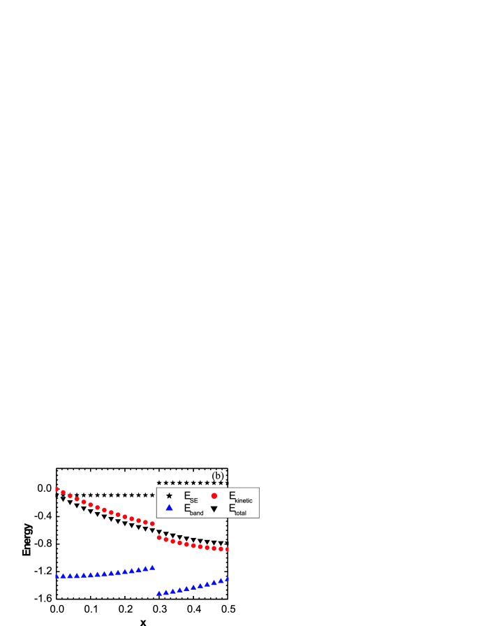
Figure 2: Results of the minimisation of Eq. (15) (with the constraint Eq. (9)): (a) Magnetic phase diagram at $T=0$. Under increasing hole doping $x$, the $C$-AF order changes via the canted Ca** phase, with spins canted on two bonds, to a homogenous FM phase. The grey horizontal line depicts the realistic value of SE $J=0.18$ in LaVO₃. Note that for $x=0$ the obtained magnetic order consists of decoupled AF $(\hat{x},\hat{y})$ planes [after Ref. [7]]; (b) Competing: correlated kinetic energy ($E_{\text{kinetic}}$), and magnetic energy ($E_{\text{SE}}$) as a function of hole doping $x$ for the fixed value of SE $J=0.18$. Kinetic energy for uncorrelated electrons ($E_{\text{band}}$) and the total energy of the system ($E_{\text{total}}$) is also shown.

4 Discussion of the results

4.1 Why Hartree-Fock approximation fails

Let us first discuss the validity of the two mean-field approximations. For the HFA we infer that for small doping ($x\rightarrow 0$) the correlated kinetic energy ($E_{\text{kinetic}}$ in Fig. 1(b)) does not tend to zero and instead equals 1/4 of the uncorrelated kinetic energy for $x=0$. This is a remnant of the fact that in the HFA the probability for existence of the hole at each site is equal to 25%. Thus, we conclude that the configurations with double occupancies are not suppressed and that HFA fails, at least in the low hole doping regime. The reason why we cannot use HFA, unlike in e.g. the undoped antiferromagnet, is that the orbital state, which is favoured here by the DE mechanism, is not an ordered state. If we were to get the FO or AO state, HFA would give physically relevant results.

4.2 Stability of the $C$-AF: generic role of the degenerate $t_{2g}$ orbitals

We concentrate on the results obtained within KRA which give the (qualitatively) right value of the correlated kinetic energy of the Hamiltonian Eq. (1), cf. Fig. 2(b). The $C$-AF order and a concomitant one-dimensional (1D) metallic state is stable for a broad range of the phase diagram parameters, in particular for the realistic value of SE $J=0.18$ and $0<x<0.28$ hole doping. This means that the DE mechanism does not win in the $(\hat{x},\hat{y})$ planes, where the SE mechanism takes over. The first explanation of this phenomenon would be to ascribe the role of the driving force for the stability of the $C$-AF order to the Coulomb repulsion $U$: the correlated kinetic energy ($E_{\text{kinetic}}$ in Fig. 2(b)) is much smaller than the bare band energy ($E_{\text{band}}$ in Fig. 1(b)) and hence the possible kinetic energy gain in the homogeneous FM state is much smaller in the correlated regime than in the conventional free electron regime. However, for hole-doped manganites $U$, $J_{H}$ and $t$ are of the same order as for hole-doped vanadates [10]. But in the manganites for $x>0.18$ hole doping the homogeneous FM order, concomitant with the metallic state, is stabilized mainly due to the DE mechanism [11]! The only difference is that in the manganites the itinerant electrons hop between degenerate $e_{g}$ orbitals and in the vanadates between degenerate $t_{2g}$ orbitals. Besides, the AF interaction between core spins is truely three-dimensional in manganites and not two-dimensional (2D) as it is the case of our model. Thus the relative weakness of the DE mechanism in the Hamiltonian Eq. (1) can be attributed to the specific features of the $t_{2g}$ electrons: the strictly 2D and strictly flavor conserving hopping between these degenerate orbitals [7].

This generic role of the $t_{2g}$ orbitals in the stability of the $C$-AF order is threefold:

(i) The AF SE interactions are rigorously 2D because for $xy$ electrons the virtual hopping processes leading to the SE interactions can happen only in the $(\hat{x},\hat{y})$ plane. Hence it makes possible: the hopping in the $\hat{z}$ direction without destruction of the magnetic order, and thus the gain of the kinetic energy without any loss in the magnetic energy. Though this is rather a specific feature of our simplified SE interactions than of the DE mechanism itself it should be stressed that the physical setting in which we can have the DE via $t_{2g}$ degenerate orbitals is such that the AF core spin interactions are 2D.

(ii) The degeneracy of the orbitals reduces the correlated kinetic energy and hence makes it energetically unfavourable to get homogenous FM order. Cf. Fig. 2(a) of Ref. [7] where for the system without orbital degeneracy with holes doped only into $zx$ orbital, i.e. with the Hamiltonian:

$$\mathcal{H}_{zx}=-u_{x}\sum_{i,j\|\hat{x}}{d}_{i}^{\dagger}{d}_{j}-\sum_{i,j\|\hat{z}}{b}_{i}^{\dagger}{b}_{j}+\frac{J}{2}L^{3}(u_{x}^{2}+u_{y}^{2}-1),$$ (16)

we obtain that for the realistic value of $J=0.18$ the FM order is already stable for hole doping $x>0.1$. Note that this comparison is valid only if the degenerate orbitals are in the OL state which indeed is the case, cf. discussion below.

(iii) Since each of the $t_{2g}$ orbitals has a different inactive axis [i.e. the cubic direction in which the electrons cannot hop] this means that if one of these orbitals is "engaged" in the AF SE interactions [cf. (i)] than the other two orbitals have one active axis in the direction perpendicular to the plane with AF bonds. Hence, hopping in the $\hat{z}$ direction, assumed in point (i), is indeed possible.

4.3 Stability of the orbital liquid

The orbital state which is concomitant with the obtained magnetic phases is the OL since: (i) we obtained $x_{a}=x_{b}$ for all of the magnetic phases, (ii) $x_{a}=x_{b}\Rightarrow\langle T_{i}^{z}\rangle\!:=\!\langle p^{\dagger}_{i}p_{i}\rangle\!-\!\langle q^{\dagger}_{i}q_{i}\rangle\!=\!0$ where $T_{i}^{z}$ is the $z$ component of the pseudospin orbital operator [9], (iii) $\langle a^{\dagger}_{i}b_{i}\rangle\!=\!\langle b^{\dagger}_{i}a_{i}\rangle\!=\!0\Rightarrow\langle T_{i}^{x}\rangle\!=\!\langle T_{i}^{y}\rangle\!=\!0$ for the $x$ and $y$ components of the pseudospin orbital operator [9]. The reason why none of the ordered state are realized in nature is twofold. Firstly, as already described, the AO state prohibits hopping due to the vanishing hopping integrals between different orbitals. This mimics the confinement of holes in the Neel AF, but stays in contrast with the behaviour of the $e_{g}$ orbitals. Thus we cannot gain any kinetic energy upon doping and this state is unphysical. Secondly, the FO state is also unphysical. A priori, due to the Pauli Principle the electrons in the polarized state can better avoid each other than in the unpolarized one. Hence the correlated kinetic energy of the FO state is enhanced in comparison with the OL, cf. Fig. 8 (with $\gamma=0$) of Ref. [9]. Though, the condition of the equilibrium for the whole system yields that the chemical potentials (Fermi energies) of the two fermionic subsystems (one with electrons in $yz$ orbitals and the other one in $zx$ orbitals) should be equal. For the FO state to be realized in nature it means that the DE mechanism should raise the bottom of one band so that the electrons can pour into the other one. However, the DE is too weak in our system and this does not happen.

4.4 Physical relevance of the model: comparison with the experiment

As already pointed out our model describes the physics present in the hole-doped cubic vanadates such as La_1-xSr_xVO₃ where the following phases were observed experimentally upon changing the hole doping $x$ in $T\rightarrow 0$: $C$-AF, AO and insulating one for $x<0.178$ hole concentration, $C$-AF and metallic one for $0.178<x<0.26$, and paramagnetic and metallic one for $0.26<x<0.327$ [12]. Rather similar phases were observed experimentally in Pr_1-xCa_xVO₃ and Nd_1-xSr_xVO₃ [12]. Hence our results stay in well agreement with the experiment, as we did not expect to explain by our model Eq. (1) the filling control metal-insulator transition present in the system, but merely the coexistence of the metallic phase, the OL state and the $C$-AF magnetic order in the above mentioned doping range. However, let us note that including the SE interactions between the itinerant electrons would stabilize the 1D OL in the $\hat{z}$ direction and AO in the $(\hat{x},\hat{y})$ plane [4]. Thus, if we included the realistic SE in the Hamiltonian Eq. (1) we would get the insulating behaviour for finite hole doping due to the AO order in the plane which would act as a string potential for holes moving in the $\hat{z}$ direction. This suggests that further investigation of the even more realistic DE model with $t_{2g}$ orbital degrees of freedom and SE interactions between itinerant electrons would not only uncover some new interesting physics but also could explain the experimentally observed phases in the doped cubic vanadates.

5 Summary

In summary, we have shown the distinct features of the double exchange via $t_{2g}$ degenerate orbitals. These features, attributed to the $t_{2g}$ orbital degeneracy, are the following:

(i) Similar to the electron-doped $e_{g}$ degenerate orbitals [6] the orbital degeneracy naturally allows for the coexistence of the anisotropic magnetic phases and the metallic phase. This is a generic feature of the DE mechanism via degenerate orbitals.

(ii) In contrast with the hole-doped $e_{g}$ case [11] the homogenous FM order is not stable for large range of doping in the discussed here hole-doped regime of $t_{2g}$ case. This is due to the different geometry of the $t_{2g}$ orbitals causing the hopping being strictly 2D and strictly flavour conserving, hence weakening the DE mechanism.

(iii) Upon hole-doping the orbitals form the OL state due to the weakness of the DE mechanism. Hence, they do not order as it is typical for the electron-doped $e_{g}$ systems [6]. However, it should be stressed that the type of the orbital state for hole-doped $e_{g}$ systems is still under discussion [9].

Besides, the correlated behaviour of the itinerant electrons plays a crucial role in the stability of the obtained magnetic and orbital phases. This is especially dramatic in the orbital sector, where the orbitals form the orbital liquid and the HFA [suitable either for weakly interacting electrons or for the ordered states] fails qualitatively in giving the right values of the kinetic energy. Altogether these are striking results which can serve as a basis for further investigation of the correlated phenomena in hole-doped systems with $t_{2g}$ orbital degeneracy.

Acknowledgments I am particularly grateful to A. M. Oleś for his invaluable idea and discussions. I would like to acknowledge support by the Polish Ministry of Science and Education under Project No. 1 P03B 068 26.

References

- [1] Y. Tokura and N. Nagaosa, Science 288, 462 (2000).
- [2] L. F. Feiner and A. M. Oleś, Phys. Rev. B 59, 3295 (1999).
- [3] M. Daghofer, A. M. Oleś, and W. von der Linden, Phys. Rev. B 70, 184430 (2004).
- [4] G. Khaliullin, P. Horsch, and A. M. Oleś, Phys. Rev. Lett. 86, 3879 (2001).
- [5] C. Zener, Phys. Rev. 82, 403 (1951).
- [6] J. van den Brink and D. I. Khomskii, Phys. Rev. Lett. 82, 1016 (1999).
- [7] K. Wohlfeld and A. M. Oleś, Phys. Stat. Sol. (b) 243, 142 (2006).
- [8] G. Kotliar and A. E. Ruckenstein, Phys. Rev. Lett. 57, 1362 (1986).
- [9] L. F. Feiner and A. M. Oleś, Phys. Rev. B 71, 144422 (2005).
- [10] T. Mizokawa and A. Fujimori, Phys. Rev. B 54, 5368 (1996).
- [11] E. Dagotto, T. Hotta, and A. Moreo, Phys. Rep. 344, 1 (2001).
- [12] J. Fujioka, S. Miyasaka, and Y. Tokura, Phys. Rev. B 72, 024460 (2005).