Berry-phase oscillations of the Kondo effect in single-molecule magnets

Abstract

We show that it is possible to topologically induce or quench the Kondo resonance in the conductance of a single-molecule magnet ($S>1/2$) strongly coupled to metallic leads. This can be achieved by applying a magnetic field perpendicular to the molecule easy axis and works for both full- and half-integer spin cases. The effect is caused by the Berry-phase interference between two quantum tunneling paths of the molecule’s spin. We have calculated the renormalized Berry-phase oscillations of the Kondo peaks as a function of the transverse magnetic field as well as the conductance of the molecule by means of the poor man’s scaling method. We propose to use a new variety of the single-molecule magnet Ni₄ for the experimental observation of this phenomenon.

The quantum tunneling of the spin of single-molecule magnets (SMMs), such as Mn₁₂ experiments ; delBarco and Fe₈ Sangregorio ; Wernsdorfer , has attracted a great deal of interest. These molecules have a large total spin, strong uniaxial anisotropy, and interact very weakly when forming a crystal. They have already been proposed for high-density magnetic storage as well as quantum computing applications app . Yet, there is much to explore in their fundamental properties. For instance, recent measurements of the magnetization in bulk Fe₈ samples (see Ref. Zener ) have observed oscillations in the tunnel splitting $\Delta E_{m,m^{\prime}}$ between states $S_{z}=m$ and $m^{\prime}$ as a function of a transverse magnetic field at temperatures between $0.05$ K and $=0.7$ K. Using a coherent spin-state path integral approach, it has been shown that this effect results from the interference between Berry phases carried by spin tunneling paths of opposite windings Loss ; Delft ; Garg , a concept also applicable to transitions involving excited states of SMMs Leuenberger_Berry .

A new approach to the study of SMMs opened up recently with the first observations of quantized electronic transport through an isolated Mn₁₂ molecule newexps . One expects a rich interplay between quantum tunneling, phase coherence, and electronic correlations in the transport properties of SMMs. It has been argued that the Kondo effect would only be observable for SMMs with half-integer spin Romeike_Kondo and therefore absent for SMMs such as Mn₁₂, Fe₈, and Ni₄, where the spin is integer. Here we show that this prediction is only valid in the absence of an external magnetic field. Remarkably, even a moderate transverse magnetic field topologically quenches the two lowest levels of a full-integer spin SMM, making them degenerate. The same Berry-phase interference also affects transport for SMMs with half-integer spin: In that case, sweeping the magnetic field will lead not to one but a series of Kondo resonances.

It is interesting to contrast the Kondo effect in a SMM with that observable in a lateral quantum dot with a single excess electron Goldhaber ; Cronenwett , in a single spin-1/2 atom Park , or in a single spin-1/2 molecule Liang . In those cases, at zero bias the Kondo effect is damped by an external a magnetic field because the degeneracy of the two spin states is lifted Glazman2005 . In the case of SMMs, the Berry-phase oscillations of the tunnel splitting $\Delta E_{m,m^{\prime}}$ leads to oscillation of the Kondo effect as a function of $H_{\bot}$, the transverse magnetic field amplitude. This means that the Kondo effect is observable at zero bias for all values of $H_{\bot,0}$ such that $\Delta E_{m,m^{\prime}}(H_{\bot,0})=0$. Notice that at a finite bias the Kondo effect in a quantum dot in the presence of a magnetic field of magnitude $H$ can be restored by tuning the bias to $eV=\pm g\mu_{B}H$ (see Ref. Goldhaber ). For SMMs, however, the interference between the Berry phases accumulated by the molecule’s spin makes the distance between the split Kondo peaks, which is equal to $eV=\pm\Delta E_{m,m^{\prime}}$, oscillate as a function of $H_{\bot}$.

Consider a typical spin Hamiltonian of a SMM in an external transverse magnetic field $H_{\bot}$:

$${\cal H}_{\rm spin} = -A_{q}S_{q,z}^{2}+\frac{B_{q}}{2}\left(S_{q,+}^{2}+S_{q,-}^{2}\right)+\frac{B_{4,q}}{3}\left(S_{q,+}^{4}+S_{q,-}^{4}\right)$$ (1)

$$+\frac{1}{2}(h_{\bot}^{*}S_{q,+}+h_{\bot}S_{q,-}),$$

where the easy axis is taken along $z$, $S_{q,\pm}=S_{q,x}\pm iS_{q,y}$, the integer index $q$ denotes the charging state of the SMM, and $h_{\bot}=g\mu_{B}H_{\bot}$. Note that the transverse magnetic field lies in the $xy$ plane. In this Hamiltonian, the dominant longitudinal anisotropy term creates a ladder structure in the molecule spectrum where the $|\pm m_{q}\rangle$ eigenstates of $S_{z}$ are degenerate. The weak transverse anisotropy terms couple these states. The coupling parameters depend on the charging state of the molecule. For example, it is known that Mn₁₂ changes its easy-axis anisotropy constant (and its total spin) from $A_{0}=56$ $\mu$eV ($S_{0}=10$) to $A_{-1}=43$ $\mu$eV ($S_{-1}=19/2$) and $A_{-2}=32$ $\mu$eV ($S_{-2}=10$) when singly and doubly charged, respectively dataexps .

The spin tunneling between the states $\left|m_{q}\right>$ to $\left|-m_{q}\right>$, with $|m_{q}|\leq S_{q}$, can occur both clockwise and counterclockwise around the $x$ axis. These two paths interfere with each other, which leads to Berry-phase oscillations Garg ; Leuenberger_Berry . Experiments with Ni₄ show that $B_{4,q=0}=-0.003$ K, i.e. $B_{4,0}$ is negative. In this case, in order to see the Berry-phase oscillation, the transverse magnetic field must be applied along angles that depend on the values of $B_{q}$ and $B_{4,q}$ Leuenberger_Berry . In Fig. 1 we show the Berry-phase oscillations of the tunnel splitting calculated for Ni₄ for two of such special orientations based on data from Ref. Sieber .

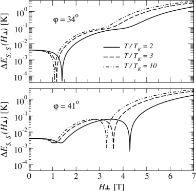
Figure 1: Berry-phase oscillations of the spin tunnel splitting in the Ni₄ spin cluster of Ref. Sieber at different temperatures ($S=4$). The anisotropy constants are $A=-1.33$ K, $B=0.034$ K, and $B_{4}^{4}=-0.003$ K. $\Delta E_{S,-S}$ is calculated by an exact diagonalization for $\varphi=33.5^{\circ}$ and $\varphi=40.75^{\circ}$. As $T$ approaches $T_{K}$, the renormalization of the $g$ factor increases, an effect that can be verified experimentally. The bare $g$ factor is $g=2.2$ for Ni₄.

In order to show how these oscillations impact transport through the SMM, we first evaluate the Kondo effect for zero bias at the zero points, where the states $\left|m_{q}\right>$ and $\left|-m_{q}\right>$ are pairwise degenerate for all $m_{q}$. In order to consider the Kondo effect for SMMs, we need to add to the spin Hamiltonian in Eq. (1) the Kondo Hamiltonian Glazman2005

$${\cal H}_{\rm K} = \sum_{k,s}\left[\xi_{k}+\frac{1}{2}(h_{\bot}^{*}s_{+}+h_{\bot}s_{-})\right]\psi_{ks}^{\dagger}\psi_{ks}+\sum_{m_{q}}\left[J_{z}^{(m_{q})}\right.$$ (2)

$$\times\left.s_{z}\Sigma_{z}^{(m_{q})}+\frac{1}{2}J_{\perp}^{(m_{q})}\left(s_{+}\Sigma_{-}^{(m_{q})}+s_{-}\Sigma_{+}^{(m_{q})}\right)\right],$$

where ${\bf s}=\sum_{k,k^{\prime},s,s^{\prime}}\psi_{ks}^{\dagger}(\mbox{\boldmath$\sigma$}_{ss^{\prime}}/2)\psi_{k^{\prime}s^{\prime}}$ and the operators $\psi_{ks}^{\dagger}$ ($\psi_{ks}$) create (annihilate) electronic states in the leads with momentum $k$, spin $s$, and energy $\xi_{k}$. $\mbox{\boldmath$\Sigma$}^{(m_{q})}$ is the pseudospin 1/2 operator acting on the states $\left|m_{q}\right>$ and $\left|-m_{q}\right>$. We define $\Sigma_{\pm}^{(m_{q})}=\Sigma_{x}^{(m_{q})}\pm i\Sigma_{y}^{(m_{q})}=\left|\pm m_{q}\right>\left<\mp m_{q}\right|$ and $\Sigma_{z}^{(m_{q})}=\left(\left|m_{q}\right>\left<m_{q}\right|-\left|-m_{q}\right>\left<-m_{q}\right|\right)/2$. The spin-flip terms in Eq. (2) induce the Kondo resonance. The exchange part, ${\cal H}_{\rm ex}$ [the second term on the right-hand side of Eq. (2)] can be derived from a generalized Anderson’s impurity model that takes into account the charging dependence of the total spin of the SMM. When the charging energy $U$ is much larger than the tunneling matrix element $t$ between the leads and the SMM, the exchange coupling can be derived in second-order perturbation theory by means of a Schrieffer-Wolff transformation SchriefferWolff , yielding

$$J_{\perp}^{(m_{q})} = \frac{2t^{2}}{U}\left[\frac{\Delta E_{m_{q-1},-m_{q-1}}}{\frac{U}{2}+\Delta E_{m_{q-1},-m_{q-1}}}+\frac{\Delta E_{m_{q+1},-m_{q+1}}}{\frac{U}{2}+\Delta E_{m_{q+1},-m_{q+1}}}\right]$$

$$\approx 4t^{2}\left(\Delta E_{m_{q-1},-m_{q-1}}+\Delta E_{m_{q+1},-m_{q+1}}\right)/U^{2},$$

$$J_{z}^{(m_{q})} = \frac{4t^{2}}{U}\left[\frac{U+\Delta E_{m_{q-1},-m_{q-1}}}{\frac{U}{2}+\Delta E_{m_{q-1},-m_{q-1}}}+\frac{U+\Delta E_{m_{q+1},-m_{q+1}}}{\frac{U}{2}+\Delta E_{m_{q+1},-m_{q+1}}}\right]$$ (3)

$$\approx 8t^{2}/U,$$

where $U$ is the charging energy. Notice that the coupling is antiferromagnetic and $J_{z}^{(m_{q})}\gg J_{\perp}^{(m_{q})}$. Since $J_{\perp}^{(m_{q})}$ depends on the tunnel splittings $\Delta E_{m_{q-1},-m_{q-1}}$ and $\Delta E_{m_{q+1},-m_{q+1}}$ (which correspond to one charge added and removed from the SMM, respectively), the Kondo exchange coupling is strongly anisotropic, which confirms the result obtained in Ref. Romeike_Kondo .

The transverse anisotropy terms in Eq. (1) mix the states $\left|m_{q}\right>$. Since $|A|\gg|B|,|B_{4}|S^{2}$, the eigenstates are nondegenerate and of the form $\left|m_{q}^{(\pm)}\right>=\left(\left|m_{q}\right>\pm\left|-m_{q}\right>\right)/\sqrt{2}$. However, at the zero points the SU(2) symmetry is restored, yielding degenerate eigenstates of the form $\left|\pm m_{q}\right>$. The Kondo Hamiltonian in Eq. (2) opens up transition paths between pairs of degenerate states $\left|m_{q}\right>$ and $\left|-m_{q}\right>$ and these paths depend on temperature. This leads in general to multi-path (but single-channel) Kondo correlations at $T>T_{K}$. At $T=0$, however, only the $\left|\pm S\right>$ states contribute to the Kondo effect. The unusual feature of Eq. (2) is that the total spin is not conserved. After a spin-flipping event, the excess angular momentum $L=2m_{q-1}\hbar$ must be absorbed by orbital (and possibly nuclear) degrees of freedom in the SMM and then be transfered to the molecule as a whole. Since the kinetic energy of a rotation of tens of $\hbar$ corresponds to a few mK for a typical SMM, the excess orbital angular momentum will be relaxed by thermal fluctuations in the metallic contacts. The critical assumption we make is that the excess angular momentum is transfered from spin to orbital (and possibly nuclear) degrees of freedom fast enough as to allow for the Kondo state to be formed.

Our analysis employs the standard poor man’s scaling Anderson to renormalize the effective exchange coupling constants $J_{z}$, $J_{+}$, $J_{-}$, and the $g$ factor. In order to make the discussion self-contained, we present the main steps of the derivation. We start by calculating the renormalization flow at the zero points where the Kondo effect is observable for zero bias. It is reasonable to assume that $h_{x,0,n}\gg T_{K}$, except when $n=0$ for half-integer spins. The total Hamiltonian for the combined SMM and leads system reads (e will suppress the index $q$ hereafter)

$${\cal H}_{\rm tot} = \sum_{m\geq 0}\left[\epsilon_{m}\left(\Sigma_{z}^{(m)}\right)^{2}+\frac{1}{2}\eta^{(m)}\left(\tilde{h}_{\bot}^{*}\Sigma_{+}^{(m)}+\tilde{h}_{\bot}\Sigma_{-}^{(m)}\right)\right]$$ (4)

$$+\sum_{k,s}\xi_{k}\psi_{ks}^{\dagger}\psi_{ks}+{\cal H}_{\rm ex},$$

where $\epsilon_{m}$ is the eigenvalue of $\left|m\right>$ and $\left|-m\right>$ at the zero points, $|\tilde{h}_{\bot}|$ is the effective Zeeman splitting between $\left(e^{-i\varphi/2}\left|m\right>+e^{i\varphi/2}\left|-m\right>\right)/\sqrt{2}$ and $\left(e^{-i\varphi/2}\left|m\right>-e^{i\varphi/2}\left|-m\right>\right)/\sqrt{2}$, and $\eta^{(m)}=1-\rho_{0}j_{\bot}^{(m)}/2$ due to the Knight shift, with $\rho_{0}$ denoting the density of states of the itinerant electrons. The Zeeman term for the itinerant electrons is absent in Eq. (4) because at finite values of $h_{\bot,0,n}$ one has to cut the edges of the spin-up and spin-down bands in the leads to make them symmetric with respect to the Fermi energy Glazman2005 . Let us call $D$ the resulting band width. The Hamiltonian remains invariant under renormalization group transformations. Using a one-loop expansion (second-order perturbation theory), we obtain the flow equations

$$\frac{dJ_{\pm}^{(m)}}{d\zeta} = -2\rho_{0}\,J_{\pm}^{(m)}J_{z}^{(m)},\qquad\frac{dJ_{z}^{(m)}}{d\zeta}=-2\rho_{0}\,J_{+}^{(m)}J_{-}^{(m)},$$ (5)

$$\frac{d\eta^{(m)}}{d\zeta} = \frac{\rho_{0}^{2}}{2}\,\left(J_{+}^{(m)}+J_{-}^{(m)}\right)J_{z}^{(m)},$$ (6)

where $\zeta=\ln(\tilde{D}/D)$ and $\tilde{D}$ is the rescaled band width. Dividing Eqs. (5) and integrating by parts gives $\left(J_{z}^{(m)}\right)^{2}-\left(J_{\bot}^{(m)}\right)^{2}=C^{(m)}$, where $C^{(m)}$ is a positive constant Anderson . The exchange coupling constants always flow to an antiferromagnetic state because $J_{z}^{(m)}>0$, but at the end of the flow the coupling tends to become isotropic. Solving Eqs. (5) yields

$$\frac{1}{2\rho_{0}\sqrt{C^{(m)}}}\,{\rm arctanh}\left(\frac{\sqrt{C^{(m)}}}{J_{z}^{(m)}}\right)=\ln\left(\frac{\tilde{D}}{T_{K}}\right).$$ (7)

The solution for $J_{\bot}^{(m)}$ is determined by $J_{z}^{(m)}=\sqrt{\left(J_{\bot}^{(m)}\right)^{2}+C^{(m)}}$. The flow stops at $\tilde{D}\approx\omega\sim T>T_{K}$. The result of the flow for $\eta$ is presented in Fig. 2.

We are now ready to calculate the linear conductance through the SMM, which is given by the formula Glazman2005

$$G=G_{0}\int d\omega\left(-\frac{df}{d\omega}\right)\frac{\pi^{2}\rho_{0}^{2}}{16}\frac{\sum_{m}e^{-\epsilon_{m}/T}\left|{\cal A}^{(m)}(\omega)\right|^{2}}{\sum_{m}e^{-\epsilon_{m}/T}},$$ (8)

where $G_{0}$ is the classical (incoherent) conductance of the molecule. At the end of the flow the transition amplitude ${\cal A}^{(m)}$ can be calculated in first-order perturbation theory and one finds that $\eta_{\tilde{D}\approx\omega}^{(m)}=1-\rho_{0}J_{\bot,\omega}^{(m)}/2$ and

$${\cal A}_{\tilde{D}\approx\omega}^{(m)} = J_{\bot,\omega}^{(m)}=\sqrt{C^{(m)}}\left[\frac{(\omega/T_{K})^{2\rho_{0}\sqrt{C^{(m)}}}}{(\omega/T_{K})^{4\rho_{0}\sqrt{C^{(m)}}}-1}\right],$$ (9)

Substituting $\omega$ by $T$ and inserting Eq. (9) into (8), one finds that the conductance diverges as $T\rightarrow T_{K}$, signaling the onset of the Kondo effect. Since $C^{(m)}>0$ the singularity in Eq. (9) differs from the usual logarithmic behavior. The Kondo effect causes a fundamental change in the SMM behavior: All the zero points of the Berry-phase oscillation get rescaled by the $g$-factor renormalization: $b_{\bot,0,n}^{(m)}=h_{\bot,0,n}/\eta_{\tilde{D}\approx T}^{(m)}$. Thus, the zero points become dependent on the contributing states $\left|m\right>$ and $\left|-m\right>$. This result indicates that the period of the Berry-phase oscillations becomes temperature dependent as $T$ is lowered toward $T_{K}$. Remarkably, the scaling equations can be checked experimentally by measuring the renormalized zero points of the Berry phase. Moreover, due to the scale invariance of the Kondo effect, the period of oscillations should follow a universal function of $T/T_{K}$.

The necessary conditions for observing these oscillations are a large enough tunnel splitting and a strong coupling between the SMM and the leads. In regard to the former, a new Ni₄ single-molecule magnet with $S=4$ has been synthesized Sieber with $\Delta E_{S,-S}\sim 0.01$ K or larger, depending on $h_{\bot}$. However, the two recent reports of transport through a SMM newexps show that the electrical contacts between the SMM and the leads is rather poor and would need to be improved in order to bring $T_{K}$ to accessible values.

Figure 2: The renormalization of the $g$ factor due to the Knight shift. As an estimate, we used $\rho_{0}J_{\pm}=\rho_{0}J_{z}=0.15$ Park .

Let us now study the linear conductance for nonzero bias, $eV=\mu_{\rm L}-\mu_{\rm R}\neq 0$. We focus on the low-temperature regime, where we can substitute $-df/d\omega$ by $\left[\delta(\omega+eV/2)-\delta(\omega-eV/2)\right]/2$ in Eq. (8). We consider the situation where one moves from the zero points $b_{\bot,0,n}$ to $b_{\bot}=b_{\bot,0,n}+\Delta b_{\bot}$, with $\Delta b_{\bot}=\eta_{b_{\bot,0,n}}\Delta h_{\bot}$. If $|eV|\ll\Delta E_{m,-m}(b_{\bot})\ll T_{K}$, the transmission amplitude is well approximated by Eq. (9). On the other hand, for $|eV|\gg T_{K}\gg\Delta E_{m,-m}(b_{\bot})$ the transmission amplitude is given by ${\cal A}_{eV}=J_{\bot,eV}$. For the case $|eV|\sim\Delta E_{m,-m}(b_{\bot})\gg T_{K}$ we can expand ${\cal A}_{\tilde{D}\approx\max\{T,\Delta E_{m,-m}(b_{\bot})\}}$ up to second order in perturbation theory at the flow end, yielding

$${\cal A}_{\tilde{D}}^{(m)}(\omega) = J_{\bot,\tilde{D}}^{(m)}+\rho_{0}J_{\bot,\tilde{D}}^{(m)}J_{z,\tilde{D}}^{(m)}\ln\left|\frac{\omega+\tilde{D}-eV/2}{\omega-\tilde{D}+eV/2}\right|,$$ (10)

where the integration limits account for the asymmetric cut of the bands. Keeping terms up to third order in $J_{\tilde{D}}^{(m)}$ and combining the results for zero and nonzero bias, we obtain

$$\frac{G}{G_{0}}=\frac{\pi^{2}\rho_{0}^{2}}{16}J_{\bot,\tilde{D}}^{2}\left[\delta_{eV,0}+\rho_{0}\,J_{z,\tilde{D}}\ln\left(\frac{\Delta E_{m,-m}}{\left||eV|-\Delta E_{m,-m}\right|}\right)\right],$$ (11)

which agrees with ref. appelbaum . The two split Kondo peaks appear at $|eV|=\Delta E_{m,-m}(b_{\bot})$. Thus, the distance between the two peaks oscillates with magnetic field, following the renormalized periodic oscillations of the tunnel splitting $\Delta E_{m,-m}(b_{\bot})$.

These results can be extended to the strong-coupling Kondo regime, namely at $T=0$, where only the two lowest-lying states $\left|S\right>$ and $\left|-S\right>$ contribute to the Kondo effect. Similarly to the spin $S=1/2$ case, our calculations yield $G(T=0)=\frac{G_{0}}{2}\sum_{s}\sin^{2}\delta_{s}=G_{0}$ at the zero points of the Berry-phase oscillation, where $|\delta_{s}|=\pi/2$ is the scattering phase shift in the unitary limit. In order to find the zero points of the Berry-phase oscillation, one must employ a more accurate approach, such as the numerical renormalization group technique future . However, since the ground state of the Kondo model given by Eq. (2) has $S_{\rm Kondo}=S_{q}-1/2$ due to the spin screening provided by the itinerant electrons, we conclude that the spin parity of the SMM effectively changes from even to odd or from odd to even when one goes from the high- to the low-temperature Kondo regimes. This means that e.g. Ni₄ should behave as if $S_{\rm Kondo}=7/2$ at $T\ll T_{K}$.

To help guide the experimental effort on this problem, we provide some estimates for the Kondo temperature using the expression $T_{K}=D\exp\left[-{\rm arctanh}\left(\sqrt{C^{(S)}}/J_{z}\right)/2\rho_{0}\sqrt{C^{(S)}}\right]$ derived from Eq. (7). Using $\rho_{0}J_{z}=0.15$ (similar to ref. Liang ) and setting $\Delta$ equal to the level spacing in the SMM, $D=|A[S^{2}-(S-1)^{2}]|=9.3$ K, we obtain $T_{K}=1.2$ K in Ni₄ for the tunneling between the ground states $m=S=4$ and $m=-S=-4$. The two crucial ingredients for the experimental observation in SMMs are: (i) a large spin tunnel splitting and (ii) a large tunneling amplitude between the leads and the SMM. The first requirement is satisfied by Ni₄. The second one remains an experimental challenge. In the case of Mn₁₂, $\Delta E_{S,-S}(H_{\bot}\sim 0)\sim 10^{-10}$ K for the ground state tunneling, which leads to a negligible small Kondo temperature $T_{K}$. However, $\Delta E_{4,-4}(H_{\bot}\sim 0)\sim 0.01$ K, which leads to $T_{K}\sim 1$ K. Unfortunately, since the excited levels $m=\pm 4$ are only populated at temperatures of about 1 K, the levels $m=\pm 4$ cannot be resolved by the electrons in the leads.

In summary, we have shown that the Kondo effect in single-molecule magnets attached to metallic electrodes is a non-monotonic (possibly periodic) function of a transverse magnetic field. This behavior is due to Berry-phase oscillations of the molecule’s large spin. The period of these oscillations is strongly renormalized near the Kondo temperature and should follow a universal function of temperature that can be accessed experimentally. We argue that a newly synthesized family of Ni₄ SMMs meets the requirements for such experiment.

This research was supported in part by the National Science Foundation under Grants No. PHY-9907949 and No. CCF-0523603. We thank E. del Barco, L. Glazman, J. Martinek, and C. Ramsey for useful discussions.

References

- (1) C. Paulsen et al., J. Magn. Magn. Mater. 140-144, 379 (1995); J. R. Friedman et al., Phys. Rev. Lett. 76, 3830 (1996); L. Thomas et al., Nature (London) 383, 145 (1996).
- (2) E. del Barco et al., J. Low Temp. Phys. 140, 119 (2005).
- (3) C. Sangregorio et al., Phys. Rev. Lett. 78, 4645 (1997).
- (4) W. Wernsdorfer and R. Sessoli, Science 284, 133 (1999).
- (5) E. Chudnovsky and L. Gunther, Phys. Rev. Lett. 60, 661 (1988); J. Tejada et al., Nanotechnology 12, 181 (2001); M. N. Leuenberger and D. Loss, Nature 410, 789 (2001).
- (6) W. Wernsdorfer et al., Europhys. Lett. 50, 552 (2000); M. N. Leuenberger and D. Loss, Phys. Rev. B 61, 12200 (2000).
- (7) D. Loss, D. P. DiVincenzo, and G. Grinstein, Phys. Rev. Lett. 69, 3232 (1992).
- (8) J. von Delft and C. L. Henley, Phys. Rev. Lett. 69, 3236 (1992).
- (9) A. Garg, Europhys. Lett. 22, 205 (1993).
- (10) M. N. Leuenberger and D. Loss, Phys. Rev. B 63, 054414 (2001).
- (11) H. B. Heersche et al., Phys. Rev. Lett. 96, 206801 (2006); M.-H. Jo et al., cond-mat/0603276.
- (12) J. R. Schrieffer and P. A. Wolff, Phys. Rev. 149, 491 (1966).
- (13) C. Romeike et al., Phys. Rev. Lett. 96, 196601 (2006).
- (14) D. Goldhaber-Gordon et al., Nature 391, 156 (1998).
- (15) S. M. Cronenwett, T. H. Oosterkamp, and L. P. Kouwenhoven, Science 281, 540 (1998).
- (16) J. Park et al., Nature 417, 722 (2002).
- (17) W. Liang et al., Nature 417, 725 (2002).
- (18) L. I. Glazman and M. Pustilnik, in Nanophysics: Coherence and Transport, 427, eds. H. Bouchiat et al. (Elsevier, 2005).
- (19) R. Basler et al., Inorg. Chem. 44, 649 (2005); N. E. Chakov et al., ibid. 44, 5304 (2005).
- (20) A. Sieber et al., Inorg. Chem. 44, 4315 (2005).
- (21) P. W. Anderson, J. Phys. C 3, 2436 (1970).
- (22) J. Appelbaum, Phys. Rev. 154, 633 (1967).
- (23) M. N. Leuenberger and E. R. Mucciolo (unpublished).