Can the Ising critical behavior survive in non-equilibrium synchronous cellular automata?

Abstract

Universality classes of Ising-like phase transitions are investigated in series of two-dimensional synchronously updated probabilistic cellular automata (PCAs), whose time evolution rules are either of Glauber type or of majority-vote type, and degrees of anisotropy are varied. Although early works showed that coupled map lattices and PCAs with synchronously updating rules belong to a universality class distinct from the Ising class, careful calculations reveal that synchronous Glauber PCAs should be categorized into the Ising class, regardless of the degree of anisotropy. Majority-vote PCAs for the system size considered yield exponents $\nu$ which are between those of the two classes, closer to the Ising value, with slight dependence on the anisotropy. The results indicate that the Ising critical behavior is robust with respect to anisotropy and synchronism for those types of non-equilibrium PCAs. There are no longer any PCAs known to belong to the non-Ising class.

1 Introduction

The concept of universality class, which has been undoubtedly one of the central issues in equilibrium physics, is widely believed to hold in some range of non-equilibrium systems [1, 2]. That is, even far from equilibrium, many microscopic details of systems become irrelevant at transition points, and a set of critical exponents depends only on a small number of basic, macroscopic ingredients. The “basic ingredients” comprise, e.g., spatial dimension, symmetries and conservation laws, as in equilibrium systems, but then it is natural to ask “do there exist any additional relevant parameters intrinsic to non-equilibrium?”

The Ising universality class is also observed in non-equilibrium systems. For example, probabilistic cellular automata (PCAs) and coupled map lattices (CMLs) with up-down symmetry can exhibit Ising-like transitions by varying a control parameter such as a coupling constant. Grinstein et al. [3] showed that, suppose a coarse-grained dynamics of such systems is described by a Langevin equation, irreversibility due to the broken detailed balance is irrelevant and the considered models should fall in the Ising class, using the standard dynamic renormalization group treatment. This prediction has been actually confirmed in various kinetic Ising models with asynchronously updating rules [4]. However, Marcq et al. [5] numerically found that Ising-like transitions of some two-dimensional non-equilibrium CMLs separate into two distinct universality classes: the Ising class, and a new universality class, called “non-Ising class” hereafter, where the correlation length exponent $\nu$ is $0.90(2)$ [here number(s) between parentheses indicate the uncertainty in the last digit(s) of the quantity], which differs from the Ising value $\nu=1$. Ratios of exponents $\beta/\nu$ and $\gamma/\nu$ are common to the two classes, namely $0.125$ and $1.75$, respectively. Since CMLs with synchronously updating rules form the new class, whereas asynchronously updated ones belong to the Ising class, synchronism is thought to be a relevant parameter. After their work, several synchronous systems such as stochastic CMLs [6], a logistic CML at the onset of a non-trivial collective behavior [7], and even PCAs [8, 9] have been investigated and the existence of the non-Ising class has been observed again, aside from a few exceptions [6, 10]. Thus the importance of synchronism, which may be related to the existence of an external clock, has been attracted much attention [11].

However, it is obvious that the synchronous updating does not immediately bring about the non-Ising critical behavior: there exist synchronous PCAs which respect the detailed balance and therefore we can safely say that they belong to the Ising class, thanks to the equilibrium universality hypothesis. For example, an isotropic PCA with a Glauber transition rate satisfies that condition. On the other hand, a Glauber PCA with completely anisotropic interaction was numerically studied by Makowiec and Gnaciński (MG) [9], and concluded to be in the non-Ising class. The above two observations naturally lead to a supposition that a degree of anisotropy may affect the selection of the universality classes. The aim of this paper is, therefore, to examine the relation between anisotropy and the universality classes.

2 Models

Two series of PCAs with up-down symmetry, namely Glauber PCAs and majority-vote PCAs, are numerically investigated. Both of them are on a two-dimensional, square lattice of size $L\times L$ with periodic boundary conditions. A local variable, or “spin,” $s_{i,j}^{t}\in\{-1,+1\}$ is assigned to each lattice point, where indices $i$ and $j$ denote Cartesian coordinates, and $t$ is the discrete time. Each site $(i,j)$ is simultaneously updated according to a specific local transition probability $p_{i,j}(\pm 1|\{s\})$ that the spin takes a value $\pm 1$ after one time step from a spin configuration $\{s\}$. For the Glauber PCAs, it is defined as

$$p_{i,j}(\pm 1|\{s\})=\frac{1}{2}\{1\pm\tanh g[s_{i,j}+s_{i+1,j}+s_{i,j-1}+\alpha(s_{i-1,j}+s_{i,j+1})]\},$$ (1)

where $g$ is a coupling constant acting as a control paramter, and $0\leq\alpha\leq 1$ indicates the degree of anisotropy. We can realize a variety of Glauber PCAs with different degrees of anisotropy by varying the value of $\alpha$. An isotropic case corresponds to $\alpha=1$, in which it is easily shown that the detailed balance is satisfied with stationary distribution $P(\{s\})\equiv\frac{1}{Z}\e^{-\mathcal{H}(\{s\})},\mathcal{H}(\{s\})=-\sum_{i,j}\ln\cosh g\left(s_{i,j}+s_{i-1,j}+s_{i+1,j}+s_{i,j-1}+s_{i,j+1}\right),$ where $\mathcal{H}(\{s\})$ is an effective Hamiltonian and $1/Z$ is a normalization constant. Since the Hamiltonian respects the up-down symmetry and consists only of short-range interactions, the equilibrium universality hypothesis asserts that this isotropic Glauber PCA should fall in the Ising class despite the synchronous updating scheme. On the other hand, the detailed balance does not hold for $\alpha\neq 1$. In particular, the completely anisotropic case $\alpha=0$ is already reported by MG to have the exponent $\nu=0.93(3)$ and to belong to the non-Ising class [9].

The other series of PCAs is that of majority-vote PCAs, defined as

$$p_{i,j}(\pm 1|\{s\})=\frac{1}{2}\{1\pm g\operatorname{sgn}[s_{i,j}+s_{i+1,j}+s_{i,j-1}+\alpha(s_{i-1,j}+s_{i,j+1})]\}.$$ (2)

For this model, the degree of anisotropy is classified into only 3 types: completely anisotropic $0\leq\alpha<0.5$, intermediate $\alpha=0.5$, and isotropic $0.5<\alpha\leq 1$. The detailed balance is violated in all of them [3, 12]. The completely anisotropic case is well-known as the Toom PCA [13], whose exponent was also estimated by MG to be $\nu=0.86(4)$, i.e. the non-Ising value [8, 9].

3 Methodology

All of the simulations are implemented on lattices of size up to $L=96$ by the following procedure. We start from random initial conditions and discard first $t_{0}=10^{5}$ time steps as transients. It is sufficiently long to consider the systems in the time-asymptotic attractor, since the correlation time is $\tau_{\text{corr}}\sim 5\times 10^{3}$ in the worst case. Then time series of the averaged spin $m_{L}^{t}\equiv(1/L^{2})\sum_{i,j}s_{i,j}^{t}$ is used to calculate the magnetization $M_{L}$, higher order moments $M_{L}^{(n)}$, the susceptibility $\chi_{L}$ and the Binder’s cumulant $U_{L}$ [14], defined by

$$M_{L}=\langle|m_{L}^{t}|\rangle,~{}~{}~{}~{}M_{L}^{(n)}=\langle|m_{L}^{t}|^{n}\rangle,~{}~{}~{}~{}$$

$$\chi_{L}=L^{2}(M_{L}^{(2)}-M_{L}^{2}),~{}~{}~{}~{}U_{L}(g)=1-\frac{M_{L}^{(4)}(g)}{3M_{L}^{(2)}(g)^{2}},$$ (3)

where $\langle\cdots\rangle$ denotes the expectation value obtained by integrating an observable during the duration $T$, such as $\langle|m_{L}^{t}|\rangle=(1/T)\sum_{t=t_{0}+1}^{t_{0}+T}|m_{L}^{t}|$. Absolute values of $m_{L}^{t}$ are taken in eqs. (3) as usual, since finite-size effects allow sign reversals of the instantaneous magnetization even in the ordered phase. The integration time $T$ is $8\times 10^{7}$ for the isotropic Glauber PCA and $1.5\times 10^{8}$ for the others, and thus much longer than both the correlation time $\tau_{\text{corr}}\lesssim 5\times 10^{3}$ and the sign reversal time $\tau_{\text{rev}}\lesssim 5\times 10^{5}$. Therefore, the quantities in eqs. (3) are capable of representing the corresponding ensemble averages with good accuracy.

4 Measurement of critical exponents

Critical exponents $\beta,\gamma,\nu$ are estimated for the Glauber PCAs with $\alpha=0$, $0.25$, $0.5$, $0.75$, $1$ and the majority-vote PCAs with $\alpha=0$, $0.5$, $1$. The way of measurement is almost similar to that of Marcq et al. and later works [5, 6, 8, 9, 10], that is, to exploit finite-size scaling laws in equilibrium which are empirically known to hold in the non-equilibrium Ising-like transitions. The following shows the process of measurement for the Glauber PCA with $\alpha=0.75$ as a typical case.

The first to do is to find the critical point $g=g_{c}$. In order to locate it, we adopt the standard method using the Binder’s cumulant $U_{L}(g)$ [14]. Since the cumulant has the scaling form of $U_{L}(g)=\hat{U}((g-g_{c})L^{1/\nu})$, it becomes independent of $L$ at criticality, i.e. $U_{L}(g_{c})=U^{*}$ for all $L$. The quantity $U^{*}$ is also a universal number. Figure 2 shows plots of $U_{L}(g)$ and their polynomial fitting curves for various system sizes.

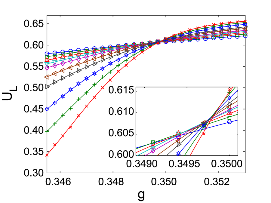
Figure 1: Plots of the Binder’s cumulant $U_{L}(g)$ for the Glauber PCA with $\alpha=0.75$. System sizes are, from the smallest slope, $L=16$, $20$, $24$, $28$, $32$, $40$, $48$, $64$, $80$, $96$. Symbols correspond to raw data and curves indicate 5th order polynomial fits. The inset is a magnification of the intersection region.

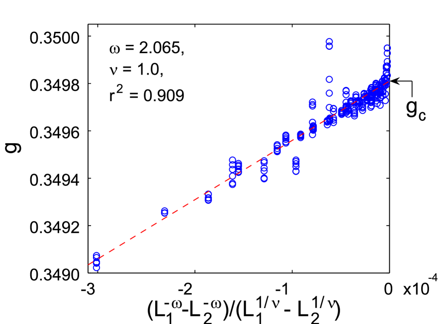
Figure 2: Plot of coordinates $g$ of intersections between curves $U_{L_{1}}(g)$ and $U_{L_{2}}(g)$. The intersections are located by fitting raw data with polynomials of orders $4$ to $9$, and superimposed on the same figure. The range of the orders is chosen so that the fitting curves adequately trace the raw data. The broken line indicates the linear regression, whose y-intercept yields an estimate of $g_{c}$. See eq. (4).

Focussing on intersections between them, a drift toward larger values of $g$ is clearly observed (the inset of fig. 2). This is caused by remaining contributions of irrelevant operators, which exist in finite-size systems [14]. Taking it into consideration, the scaling function of the cumulant should be modified to $U_{L}(g)=\hat{U}((g-g_{c})L^{1/\nu},\mathcal{O}L^{-\omega})$, where only one irrelevant term with a relaxation exponent $\omega$ is assumed to be dominant. An expansion of the modified scaling form in powers of $(g-g_{c})L^{1/\nu}$ and $L^{-\omega}$ up to the 1st order yields the coordinate of the intersection between $U_{L_{1}}(g)$ and $U_{L_{2}}(g)$, namely,

$$g=g_{c}+A\frac{L_{1}^{-\omega}-L_{2}^{-\omega}}{L_{1}^{1/\nu}-L_{2}^{1/\nu}},~{}~{}~{}~{}U=U^{*}+B\frac{L_{1}^{1/\nu}L_{2}^{-\omega}-L_{2}^{1/\nu}L_{1}^{-\omega}}{L_{1}^{1/\nu}-L_{2}^{1/\nu}},$$ (4)

where $A$ and $B$ are expansion coefficients. Consequently, by plotting $g$ with respect to $(L_{1}^{-\omega}-L_{2}^{-\omega})/(L_{1}^{1/\nu}-L_{2}^{1/\nu})$ for fixed, reasonable values of $\omega$ and $\nu$, and by searching for $\omega$ which gives the highest correlation coefficient for it, we obtain estimates of both $\omega$ and $g_{c}$. Figure 2 is a plot for $\nu=1$ and the best value of $\omega$, where we can clearly see the linear dependence, which gives the coefficient of determination $r^{2}=0.909$. The critical point $g_{c}$ is then estimated as a y-intercept of the regression line, $g_{c}=0.34981^{+(4)}_{-(3)}$ in this case. Here, the superscript (subscript) indicates the confidence interval in the plus (minus) direction, which is evaluated as the region with sufficiently large coefficient of determination, namely, $(1-r^{2})<(1-\max_{\omega}r^{2})\times 1.1$. The estimation of $U^{*}$ is carried out quite similarly, which results in $U^{*}=0.6107^{+(41)}_{-(13)}$. This is in good agreement with the 2D-Ising value $U^{*}=0.611(1)$ [15]. A problem of this method may be that it requires the value of $\nu$, which is measured later, but the difference in the estimates with respect to the assumed value of $\nu$, $1.0$ or $0.9$, turns out to be quite subtle: $2\times 10^{-6}$ for $g_{c}$ and $2\times 10^{-5}$ for $U^{*}$, i.e. negligible. The mentioned improvement is therefore useful and expected to lead to more reliable estimation of critical exponents.

Now we proceed to the measurement of critical exponents. The following finite-size scaling relations are made use of to achieve it:

$$\partial_{g}\ln M_{L}|_{g_{c}}\sim L^{1/\nu}, \partial_{g}\ln M_{L}^{(2)}|_{g_{c}}\sim L^{1/\nu},$$

$$\partial_{g}\ln M_{L}^{(4)}|_{g_{c}}\sim L^{1/\nu}, \partial_{g}U_{L}|_{g_{c}}\sim L^{1/\nu},$$

$$V_{2}\equiv[m^{2}]^{2}/[m^{4}]\sim L^{1/\nu}, V_{4}\equiv([m]^{4}/[m^{4}])^{1/3}\sim L^{1/\nu},$$

$$V_{6}\equiv[m]^{2}/[m^{2}]\sim L^{1/\nu},$$ (5a)

and

$$M_{L}(g_{c})\sim L^{-\beta/\nu}, M_{L}^{(2)}(g_{c})^{1/2}\sim L^{-\beta/\nu},$$

$$M_{L}^{(4)}(g_{c})^{1/4}\sim L^{-\beta/\nu}, \chi_{L}(g_{c})\sim L^{\gamma/\nu},$$ (5b)

where $[m^{n}]\equiv\partial_{g}M_{L}^{(n)}|_{g_{c}}$, and the derivatives are evaluated by using polynomial fittings of appropriate orders. Irrelevant operators can affect the scaling relations (5) again. We, therefore, perform the measurement as follows. (I) First, we plot a quantity in eqs. (5) in the log-log scale, using a polynomial fit of a fixed order, and check the linear dependence. (IIa) If the contributions of irrelevant fields are already suppressed for the smallest size considered, $L=16$, a simple linear fit giving the lowest chi-square in the log-log plot yields an estimate. (IIb) Otherwise, finite-size corrections are employed to achieve an asymptotic value of the slope, after Marcq et al. and subsequent works [5, 6]. An expansion is made similar to that used for $U_{L}(g)$ above, e.g. $L^{-1/\nu}\partial_{g}\ln M_{L}|_{g_{c}}\simeq C_{1}+C_{2}L^{-\omega}$, followed by searching for the best $\omega$ and $\nu$ (or other exponents), in the sense of lowest chi-square. This method, however, does not work sometimes due to rapid convergence of correction terms, or statistical errors in the raw data. In that case, (IIc) we use a linear fit in the log-log plot neglecting data points subject to the finite-size effect. Care is taken to ensure that the observed scaling behavior does indeed correspond to the asymptotic regime, in all of the cases. Finally, (III) we repeat the aforesaid procedure for polynomial fits of different orders in (I), and also for all of the quantities in eqs. (5) which give the same exponent.

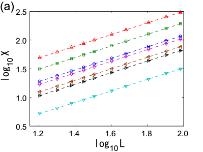
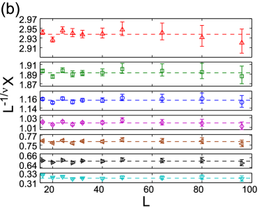
Figure 3: (a) Scaling relations of the 7 quantities in eq. (5a) for the Glauber PCA with $\alpha=0.75$, where $X=\partial_{g}\ln M_{L}^{(4)}|_{g_{c}}$, $\partial_{g}\ln M_{L}^{(2)}|_{g_{c}}$, $\partial_{g}\ln M_{L}|_{g_{c}}$, $V_{2}$, $V_{4}$, $V_{6}$, $\partial_{g}U_{L}|_{g_{c}}$ from top to bottom. Corresponding slopes are $1.017$, $1.013$, $1.011$, $1.014$, $1.012$, $1.011$ and $1.006$, respectively. (b) Deviations from the scaling laws, which are found to be faint. Note that the scale in the y-axis is identical for all of the subplots.

A value of $\nu$ for the Glauber PCA with $\alpha=0.75$ is thereby evaluated to be $\nu=0.988^{+(19)}_{-(15)}$, as is shown in fig. 3. The main sources of errors are the uncertainty in the estimate of the critical point $g_{c}$ and statistical errors due to the finite-time sampling. The former is estimated from the confidence interval of $g_{c}$, while the latter is from the dependence of exponents on the quantity used for the finite-size scaling, and on the degree of the fitting polynomials. Note that the final range of errors is given as the union of each error region considered, i.e. as wide as possible. Recalling the value of $\nu$ for the Ising and non-Ising class, $1$ and $0.90(2)$ respectively, we can clearly conclude that the Glauber PCA with $\alpha=0.75$ belongs to the Ising class. Values of $\beta/\nu$ and $\gamma/\nu$ are obtained in the same way, which are $\beta/\nu=0.1271^{+(17)}_{-(28)}$ and $\gamma/\nu=1.749^{+(15)}_{-(14)}$, and again completely consistent with the Ising values.

5 Results and discussions

Critical exponents of all of the models considered are measured in the same manner, except for the following two points. (i) Systems of size $L=16$, $20$, $24$, $28$, $32$, $40$, $48$, $64$, $80$, $96$ are examined for the Glauber PCAs with $\alpha=0.25$ and $0.75$, while those of size $L=16$, $24$, $32$, $40$, $48$, $64$, $80$, $96$ are considered for the others, since finite-size corrections are appropriately caught by them. (ii) Since no finite-size effects are observed in intersections of $U_{L}(g)$ for the Glauber PCA with $\alpha=0$, values and errors of $g_{c}$ and $U^{*}$ are determined by means and standard deviations of the coordinates of the intersections.

The measured exponents are summarized in table 1. Our results for the Glauber PCAs clearly show that they fall into the Ising class. While the isotropic case $\alpha=1$, which is at equilibrium, should actually be there, the results for all the anisotropic Glauber PCAs are quite unexpected since they are non-equilibrium, synchronous PCAs. In particular, we obtain a value of the exponent for the completely anisotropic case $\alpha=0$ as $\nu=0.992^{+(28)}_{-(26)}$ (fig. 5), which conflicts with the estimate by MG, $\nu=0.93(3)$ [9].

Table 1: Critical points and exponents of the PCAs examined.

model	$\alpha$	$g_{c}$	$U^{*}$	$\beta/\nu$	$\gamma/\nu$	$\nu$
	$1$	$0.31173^{+(6)}_{-(3)}$	$0.6098^{+(14)}_{-(5)}$	$0.1271^{+(17)}_{-(54)}$	$1.757^{+(11)}_{-(28)}$	$0.993^{+(48)}_{-(18)}$
	$0.75$	$0.34981^{+(4)}_{-(3)}$	$0.6107^{+(41)}_{-(13)}$	$0.1271^{+(17)}_{-(28)}$	$1.749^{+(15)}_{-(14)}$	$0.988^{+(19)}_{-(15)}$
Glauber	$0.5$	$0.40407^{+(6)}_{-(3)}$	$0.6100^{+(20)}_{-(7)}$	$0.1254^{+(18)}_{-(42)}$	$1.757^{+(7)}_{-(26)}$	$0.994^{+(24)}_{-(15)}$
	$0.25$	$0.49049^{+(5)}_{-(3)}$	$0.6097^{+(6)}_{-(2)}$	$0.1266^{+(10)}_{-(21)}$	$1.753^{+(10)}_{-(11)}$	$0.994^{+(22)}_{-(16)}$
	$0$	$0.65855^{+(16)}_{-(16)}$	$0.6123^{+(17)}_{-(16)}$	$0.1239^{+(32)}_{-(32)}$	$1.753^{+(11)}_{-(12)}$	$0.992^{+(28)}_{-(26)}$
	$1$	$0.73151^{+(4)}_{-(4)}$	$0.6105^{+(7)}_{-(4)}$	$0.1247^{+(15)}_{-(17)}$	$1.753^{+(12)}_{-(9)}$	$0.979^{+(27)}_{-(17)}$
majority-vote	$0.5$	$0.783324^{+(21)}_{-(17)}$	$0.6104^{+(4)}_{-(3)}$	$0.1260^{+(25)}_{-(12)}$	$1.753^{+(7)}_{-(7)}$	$0.962^{+(24)}_{-(10)}$
	$0$	$0.82248^{+(3)}_{-(2)}$	$0.6140^{+(29)}_{-(14)}$	$0.1249^{+(18)}_{-(24)}$	$1.740^{+(10)}_{-(11)}$	$0.956^{+(28)}_{-(15)}$
Ising [15]			$0.611(1)$	$0.125$	$1.75$	$1$
non-Ising [5, 6]			$\approx 0.611$	$\approx 0.125$	$\approx 1.75$	$0.90(2)$

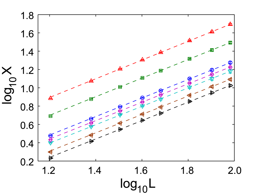
Figure 4: Measurement of the critical exponent $\nu$ for the Glauber PCA with $\alpha=0$. Each symbol and line corresponds to $X=\partial_{g}\ln M_{L}^{(4)}|_{g_{c}}$, $\partial_{g}\ln M_{L}^{(2)}|_{g_{c}}$, $\partial_{g}\ln M_{L}|_{g_{c}}$, $V_{2}$, $\partial_{g}U_{L}|_{g_{c}}$, $V_{4}$, $V_{6}$ from top to bottom. Slopes are $1.023$, $1.016$, $1.012$, $1.005$, $1.005$, $1.005$ and $1.005$, respectively.

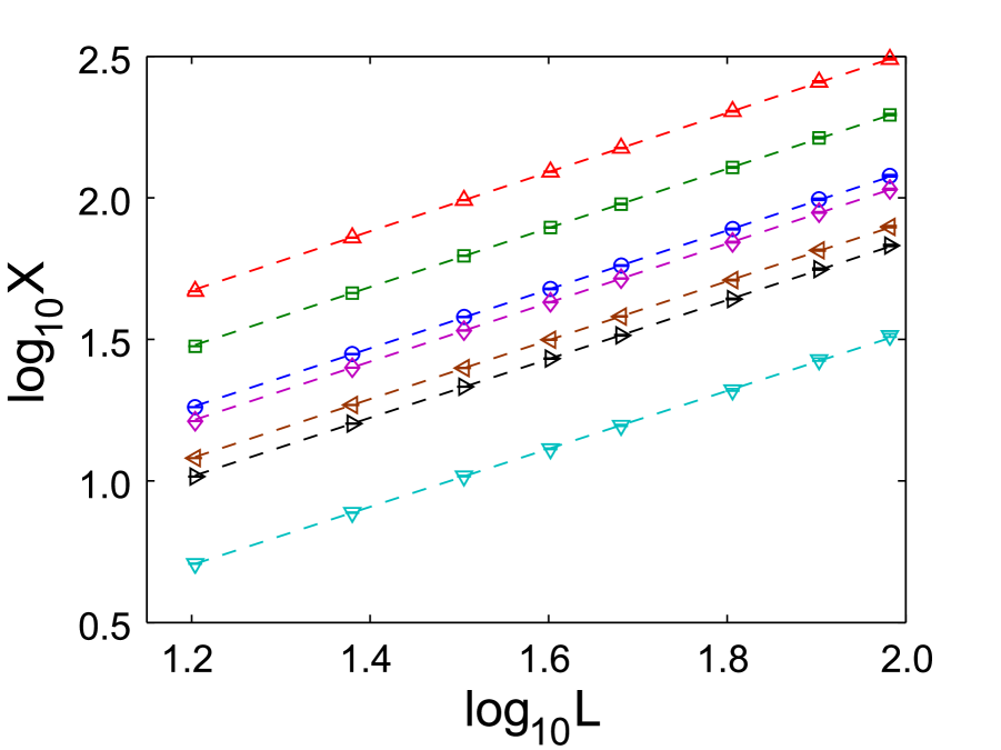
Figure 5: Measurement of the critical exponent $\nu$ for the majority-vote PCA with $\alpha=0$. Each symbol and line corresponds to $X=\partial_{g}\ln M_{L}^{(4)}|_{g_{c}}$, $\partial_{g}\ln M_{L}^{(2)}|_{g_{c}}$, $\partial_{g}\ln M_{L}|_{g_{c}}$, $V_{2}$, $V_{4}$, $V_{6}$, $\partial_{g}U_{L}|_{g_{c}}$ from top to bottom. Slopes are $1.046$, $1.044$, $1.041$, $1.044$, $1.041$, $1.039$ and $1.026$, respectively.

On the other hand, the results for the majority-vote PCAs are rather unclear: the estimated exponents $\nu$ are between the Ising and non-Ising value. They are closer to the Ising exponent and this tendency slightly increases with isotropy. There seem to be two possible interpretations for it. One is that the critical exponents of the majority-vote PCAs depend continuously on system parameters, anisotropy in our demonstrations. This is, however, commonly understood as an exceptional case, at least in equilibrium. Instead, it is rather natural to consider that what we see here is a part of an extremely slow convergence in finite-size scalings toward the Ising asymptotic behavior, which is estimated to be reached for $L\sim O(10^{4})$. The slight dependence on the degree of anisotropy is then related to the difference in relaxation constants, which may be attributed to coupling intensity between sites, and/or an additional length scale caused by some hidden coherent structures such as in [16], if they exist. In any case, further studies are essential to give a conclusion on it. In addition, the estimate for the completely anisotropic majority-vote PCA, or the Toom PCA, $\nu=0.956^{+(28)}_{-(15)}$ (fig. 5) is again incompatible with the value from MG, $\nu=0.86(4)$ [8, 9].

The discrepancies between our estimates and MG’s are caused by a few differences in steps toward estimation. One is in the sampling method. We started from random initial conditions and sampled $T=1.5\times 10^{8}$ consecutive data after discarding first $t_{0}=10^{5}$ time steps, whereas MG chose ordered initial conditions, in which all spins are $+1$, and set $t_{0}\leq 10^{4},T=10^{4}$ as the price for repeating independent simulations not more than $5500$ times. Since $t_{0}$ and $T$ of MG are in many cases comparable with the correlation time $\tau_{\text{corr}}\lesssim 5\times 10^{3}$, and comparable with or much shorter than the sign reversal time $\tau_{\text{rev}}\lesssim 5\times 10^{5}$, we consider that the sampling in MG is statistically insufficient and the influence from the ordered initial conditions may remain. Another origin of the discrepancies is a way to determine transition points $g_{c}$. We estimated them solely from the crossings of the cumulant $U_{L}(g)$, with finite-size corrections if possible, while MG first made a guess from the crossings and then determined them by searching for $g_{c}$ which gives the ratios of exponents $\beta/\nu$ and $\gamma/\nu$ identical to those of the Ising class. This is, however, rather perilous since estimates of critical exponents are very sensitive to various errors, including statistical ones. Moreover, in general, a small uncertainty in critical points $g_{c}$ leads to much larger errors in critical exponents. In fact, if we assume the value of $g_{c}$ in MG for the Glauber PCA with $\alpha=0$, namely $g_{c}=0.6580$, we reproduce their result $\nu\approx 0.93$. For the reasons above, we believe our results are more reliable.

In conclusion, we have investigated the Ising-like phase transitions in synchronous PCAs, namely the Glauber PCAs and the majority-vote PCAs, with different degrees of anisotropy. Our calculations reveal that the Glauber PCAs belong to the Ising class regardless of the degree of anisotropy, and the majority-vote PCAs are also expected to do so, though the latter remains to be clearly shown. The results indicate that the Ising critical behavior is robust with respect to anisotropy and synchronism for the PCAs, which coincide with the theoretical prediction of Grinstein et al. [3] and observations by Sastre and Pérez where some degree of deterministic dynamics is required to bring about the non-Ising critical behavior [6].

References

- [1] G. Ódor, Rev. Mod. Phys. 76, 663 (2004).
- [2] H. Hinrichsen, Adv. Phys. 49, 815 (2000).
- [3] G. Grinstein, C. Jayaprakash and Y. He, Phys. Rev. Lett. 55, 2527(1985).
- [4] See, e.g., ref. [1] section III. A.
- [5] P. Marcq, H. Chaté and P. Manneville, Phys. Rev. Lett. 77, 4003 (1996); Phys. Rev. E 55, 2606 (1997).
- [6] F. Sastre and G. Pérez, Phys. Rev. E 64, 016207 (2001).
- [7] P. Marcq, H. Chaté and P. Manneville, Prog. Theor. Phys. Suppl. 161, 244 (2006).
- [8] D. Makowiec, Phys. Rev. E 60, 3787 (1999).
- [9] D. Makowiec and P. Gnaciński, in: Proceedings of the 5th International Conference on Cellular Automata for Research and Industry, Lecture Notes in Computer Science Vol. 2493, edited by S. Bandini, B. Chopard and M. Tomassini, Springer-Verlag (Berlin, Heidelberg, 2002), p. 104.
- [10] G. Pérez, F. Sastre and R. Medina, Physica D 168, 318 (2002).
- [11] See also, e.g., H. Atmanspacher, T. Filk and H. Scheingraber, Eur. Phys. J. B 44, 229 (2005), and references therein.
- [12] J. L. Lebowitz, C. Maes and E. R. Speer, J. Stat. Phys. 59, 117 (1990).
- [13] See, e.g., A. L. Toom, N. B. Vasilyev, O. N. Stavskaya, L. G. Mityushin, G. L. Kurdyumov and S. A. Prigorov, in: Stochastic Cellular Systems: Ergodicity, Memory, Morphogenesis, edited by R. L. Dobrushin, V. I. Kryukov and A. L. Toom, Manchester University Press (Manchester, 1990), p. 1, and references therein.
- [14] K. Binder, Z. Phys. B 43, 119 (1980).
- [15] V. Privman, P. C. Hohenberg and A. Aharony, in: Phase Transitions and Critical Phenomena Vol. 14, edited by C. Domb and J. L. Lebowitz, Academic Press (London, 1991), p. 1.
- [16] P. Grassberger and T. Schreiber, Physica D 50, 177 (1991).