Ground-state Properties of Small-Size Nonlinear Dynamical Lattices

Abstract

We investigate the ground state of a system of interacting particles in small nonlinear lattices with $M\geq 3$ sites, using as a prototypical example the discrete nonlinear Schrödinger equation that has been recently used extensively in the contexts of nonlinear optics of waveguide arrays, and Bose-Einstein condensates in optical lattices. We find that, in the presence of attractive interactions, the dynamical scenario relevant to the ground state and the lowest-energy modes of such few-site nonlinear lattices reveals a variety of nontrivial features that are absent in the large/infinite lattice limits: the single-pulse solution and the uniform solution are found to coexist in a finite range of the lattice intersite coupling where, depending on the latter, one of them represents the ground state; in addition, the single-pulse mode does not even exist beyond a critical parametric threshold. Finally, the onset of the ground state (modulational) instability appears to be intimately connected with a non-standard (“double transcritical”) type of bifurcation that, to the best of our knowledge, has not been reported previously in other physical systems.

I Introduction

In the past few years, there has been a tremendous increase in the number of studies of lattice dynamical systems, especially in the context of differential-difference equations, where the evolution variable is continuum and the spatial dependence is inherently or effectively posed on a lattice reviews . Such settings appear to be ubiquitous in very diverse physical contexts ranging from the spatial dynamics of optical beams in coupled waveguide arrays in nonlinear optics reviews1 to the dynamical behavior of Bose-Einstein condensates (BECs) in optical lattices in soft-condensed matter physics reviews2 , and even the DNA double strand in biophysics reviews3 , among others.

One of the principal foci of this research effort is the analysis of the features of the localized, solitary wave solutions of such lattices. Discrete solitons solit , and various more exotic structures such as dipole solitons, soliton-trains, soliton-necklaces and vector solitons were recently observed in optical contexts such as photorefractive materials esolit . At the same time, experimental developments in the physics of BECs closely follow with prominent recent results, including the observation of bright, dark and gap solitons in quasi-one-dimensional settings bec .

Another trend that has recently been followed is to study small lattices, such as those pertaining to double or triple-well potentials. The aim there is to better understand the underlying physics of such simpler dynamical systems and subsequently explore how much of the relevant phenomenology may persist in the infinite lattice limit. It is interesting to note that few-site lattices were among the first ones to be explored thoroughly, starting with the pioneering work of eilbeck . Since then, a variety of theoretical works also examined features relevant especially to double-well (such as symmetry-breaking weinstein ), triple-well (such as oscillatory instabilities johansson and chaotic behavior penna , among others), or even multi- (but few-) well potentials (such as synchronization pando ). Most of the above studies were done in the prototypical nonlinear envelope wave equation that is equally applicable to each of the above mentioned physical settings (in appropriate parameter regimes), namely the discrete nonlinear Schrödinger equation (DNLS).

In that vein, recent experiments in both optical media zhigang and in BECs markus2 have revealed a host of interesting phenomena such as symmetry breaking in double-well potentials, and constructive (destructive) interference of in (out-of-) phase pulses in triple-well media, among others. More generally, few-site lattices such as those we are going to address in what follows appear to be within the reach of state-of-art technology in optically trapped BECs. Actually, Ref. A:Albiez reports on the analysis of the evolution of the density distribution and relative phase of a boson Josephson junction. Such a two-site system was realized by isolating a single “edge” of an optical lattice via an additional confining potential. Likewise, single “plaquettes” of suitable two-dimensional — possibly quasiperiodic — lattices rings1 can be used to create few-site closed rings. A further interesting proposal is based on transverse electromagnetic modes of laser beams rings2 .

Our main focus here is on the ground-state properties of a system of interacting particles, hopping in a few-site lattice, described by the DNLS equation. We emphasize that this is an important issue for any low- (virtually zero-) temperature system, in particular for ultracold bosons. In this respect, on lattices, the mean-field description in terms of the DNLS equations, which results from a variational approach to the quantum ground-state, proved to be quite satisfactory with both repulsive ampe and attractive interactions praBPV ; jack . Naturally, a great deal of the relevant phenomenology has been analyzed. However, we hope to illustrate that there some of the properties of low energy states are still unexplored and yet are particularly intriguing in simple and interesting systems such as the few-site lattices. As is well known, in the case of attractive, “focusing” interaction, the ground state of the homogeneous systems under investigation exhibits a delocalization transition reviews driven by the effective intersite coupling $\epsilon$. The threshold for localization is in general identified with the occurrence of modulational instability in the uniform ground state characterizing the system at large values of $\epsilon$. Here we show that this identification applies only to sufficiently large lattices. Conversely, on small lattices, these two thresholds are distinct, the delocalization transition occurring at a larger value of $\epsilon$. As we will illustrate, this feature can be understood in terms of the complex interplay of three low-energy solutions to the DNLS equations governing the system. These are the uniform state and two localized solutions that, for reasons that will become clear shortly, we refer to as single-pulse and two-pulse state, respectively. These two localized solutions emerge as excited states from a saddle-node bifurcation point below some threshold in $\epsilon$. As this parameter is further lowered below the delocalization threshold, the symmetry-breaking single-pulse state becomes the ground state of the system, but this does not influence the stability properties of the uniform state. As we will show, this feature can be in principle exploited to access metastable states of the system. Lowering $\epsilon$ further eventually results in the uniform-state modulational instability, caused by a bifurcation involving the uniform state and the two-pulse state. As we discuss in Section V, this critical point, which we dub double transcritical bifurcation, exhibits non-standard features which, to the best of our knowledge, have not been observed previously.

The layout of the paper is the following. In section II we introduce the model and recall the known results about its ground state. In Section III we show that interesting insight in the bifurcations involving the uniform state can be gained through a simple perturbative approach. In Section IV this analytical insight is fully developed for the case of the three-site lattice. Section V contains the numerical results for lattices comprising of $M=3,4,5$ sites. In particular, we discuss the non trivial features of the double transcritical bifurcation related to the uniform-state modulational instability, and illustrate how the known situation for large lattices is recovered for $M\geq 6$. Our conclusions are given in Sec. VI.

II Setup

In the following, we consider the standard DNLS equation on a $M$-site one-dimensional closed lattice,

$$i\dot{z}_{n}=-T\Delta_{2}z_{n}-\Gamma|z_{n}|^{2}z_{n},$$ (1)

where $\Delta_{2}z_{n}=(z_{n+1}+z_{n-1}-2z_{n})$ is the discrete Laplacian, and periodic boundary conditions are implemented by identifying sites $n=1$ and $n=M+1$. This equation is derived from the Hamiltonian

$$H=\sum_{n=1}^{M}T|z_{n+1}-z_{n}|^{2}-\frac{\Gamma}{2}|z_{n}|^{4}$$ (2)

making use of the standard Poisson brackets $\{z_{n},z_{m}\}=i\delta_{nm}$ reviews . We recall that Hamiltonian (2) is the semiclassical counterpart of the Bose-Hubbard model standardly adopted for describing ultracold bosonic atoms trapped in optical lattices fisher ; jaksch . In more detail, Eq. (2) is obtained by approximating the quantum states with suitable coherent states and subsequently implementing a standard variational method. Direct comparison shows that Hamiltonian (2) provides a description of the ground state properties of the fully quantum model that is satisfactory in many respects, both in the case of repulsive ampe and attractive interactions praBPV . We also recall that in this framework $T$ and $\Gamma$ — denoting the intersite coupling across adjacent sites and the boson-boson interaction, respectively — are directly related to experimental parameters that can be varied over a wide range of values jaksch ; theis . As to $z_{n}$, it is a macroscopic complex variable describing the bosonic population, $|z_{n}|^{2}$, and phase, $\arg(z_{n})$, at lattice site $n$. It is easy to prove that the total population $N=\sum_{n=1}^{M}|z_{n}|^{2}$ is conserved along the dynamics note1 .

As we mention in Sec. I, we focus on the case of attractive interactions, $\Gamma>0$. Before proceeding with our discussion, we observe that the only independent parameter in Eq. (1) other than the lattice size $M$ is the effective (rescaled) intersite coupling, $\epsilon=T/(\Gamma N)$. Actually, Eq. (1) can be recast in the form

$$i\dot{u}_{n}=-\epsilon\Delta_{2}u_{n}-|u_{n}|^{2}u_{n},$$ (3)

where $u_{n}=z_{n}/\sqrt{N}$ and the dot now denotes the derivative with respect to the rescaled time variable $t^{\prime}=\Gamma Nt$.

We are interested in the ground state of the Hamiltonian (2), i.e. in the state $v_{n}$ minimizing

$$E=\frac{H}{\Gamma N^{2}}=\sum_{n=1}^{M}\epsilon|v_{n+1}-v_{n}|^{2}-\frac{1}{2}|v_{n}|^{4}$$ (4)

Therefore $v_{n}$ satisfies the equation

$$G(v_{n};\epsilon)=\Lambda v_{n}-\epsilon\Delta_{2}v_{n}-|v_{n}|^{2}v_{n}=0.$$ (5)

where the eigenvalue $\Lambda$ is a Lagrange multiplier taking into account the constraint $\sum_{n}|v_{n}|^{2}=\sum_{n}|u_{n}|^{2}=1$ stemming from the norm conservation. We note that the solutions to the nonlinear eigenvalue problem Eq. (5) correspond to the standing wave solutions to Eq. (3) of the form $u_{n}=v_{n}e^{i\Lambda t^{\prime}}$.

Let us now recall some well known facts about this ground state. For small values of the intersite coupling $\epsilon$, the ground state of the system is known to break the translational invariance of $H$. Actually for vanishing $\epsilon$’s, i.e., in the so-called anticontinuum limit, it is easy to check that the ground state is completely localized at a single lattice site $n_{0}$, $u_{n}=\delta_{n\,n_{0}}$. As the intersite coupling is increased, the width of the localization peak increases while maintaining its single-pulse profile, i.e. remaining mirror-symmetric with respect to the central site $n_{0}$, $u_{n_{0}+k}=u_{n_{0}-k}$. Hence we refer to this solution of Eq. (5) as single-pulse state. Note that the localization peak of the single pulse state can be centered at any lattice site, so that the symmetry breaking ground-state is $M$-fold degenerate.

Conversely, for sufficiently large values of $\epsilon$, the translational symmetry is recovered, the ground state being the uniform (i.e. delocalized) state $v_{n}=v=M^{-1/2}$, of energy $E=1/(2M)$. The (finite) critical value of the intersite coupling at which the inversion in the nature of the ground state occurs is referred to as delocalization threshold. This critical value is usually identified with the threshold below which the uniform state becomes modulationally unstable jack ,

$$\epsilon_{1}(M)=\frac{1}{2M}\frac{1}{\sin^{2}\left(\frac{\pi}{M}\right)}.$$ (6)

In the following we will show that this identification is correct only for $M\geq 6$, whereas on smaller lattices the delocalization threshold occurs at a critical value $\epsilon_{2}>\epsilon_{1}(M)$. Furthermore we will show that the threshold for modulational instability corresponds to a non-standard bifurcation involving the uniform state and a low-energy localized solution to Eq. (5). We will refer to the latter as two-pulse state since, unlike the single-pulse state, its localization peak features a maximum at two adjacent sites, reducing to $u_{n}=(\delta_{n\,m}+\delta_{n\,m+1})/\sqrt{2}$ in the anticontinuum limit.

III Perturbative Approach

In this section we focus on the possible bifurcations involving the uniform state $v_{n}=1/\sqrt{M}$, which is the ground-state of the system for sufficiently large $\epsilon$’s. Hence we look for nonuniform solutions to Eq. (5) that become uniform as the intersite coupling $\epsilon$ approaches a finite value. Adopting a simple perturbative approach, we introduce a linear parameter $\tau$ such that $\epsilon=\alpha_{\epsilon}+\beta_{\epsilon}\tau$ and assume that states of the form $v_{n}=v+\tau(p_{n}+iq_{n})$ satisfy Eq. (5) with $\Lambda=v^{2}+\beta_{\Lambda}\tau$. After some simple manipulations one gets

$$\beta_{\Lambda}v-\alpha_{\epsilon}\Delta_{2}p_{n}-2v^{2}p_{n} = 0$$ (7)

$$\alpha_{\epsilon}\Delta_{2}q_{n} = 0$$ (8)

According to Eq. (8), the imaginary part of the perturbation is uniform, $q_{n}=q$. Hence, it can be absorbed in the unperturbed uniform state as a phase factor, $v\to|v|e^{i\theta}$, with $\theta=\arcsin(\tau q/|v|)$. As to the real part, it is easy to prove that the coefficient $\beta_{\Lambda}$ appearing in Eq. (7) must vanish, which suggests that spatially modulated solutions branch-off tangentially from the uniform state. This is obtained summing Eq. (7) over $n$ and making use of the constraint $\sum_{n}p_{n}=0$ stemming at linear order from the normalization for the perturbed solution, $\sum_{n}|v_{n}|^{2}=1$. Hence Eq. (7) is formally equivalent to the eigenvalue equation for the discrete Laplacian operator

$$\Delta_{2}p_{n}=\lambda p_{n},\qquad\lambda=-\frac{2v^{2}}{\alpha_{\epsilon}}=-\frac{2}{M\alpha_{\epsilon}}$$ (9)

On a $M$-site homogeneous one-dimensional lattice such as that under investigation, the Laplacian features $M$ eigenvalues of the form $\lambda_{k}=-4\sin^{2}(\pi k/M)$, with $k=0,\ldots,M-1$. These define a set of critical values for the intersite coupling, $\alpha_{\epsilon}^{(k)}=[2M\sin^{2}(\pi k/M)]^{-1}$, where nonuniform solutions become uniform. The relevant perturbative modulations have the form $p_{n}^{(k)}\propto\sin(2\pi kn/M+\varphi)$, where $\varphi$ is a phase that ensures that two solutions corresponding to the same $k$ are independent. Note that $k=0$ must be discarded, since it corresponds to a vanishing perturbation, and that $\alpha_{\epsilon}^{(k)}=\alpha_{\epsilon}^{(-k)}=\alpha_{\epsilon}^{(M-k)}$. Hence, according to this picture, one expects $\lfloor(M-1)/2\rfloor$ distinct critical values, where $\lfloor x\rfloor$ denotes the largest integer smaller than $x$.

We now observe that $\alpha_{\epsilon}^{(k+1)}<\alpha_{\epsilon}^{(k)}$, and that the largest critical value $\alpha_{\epsilon}^{(1)}$ coincides with the known threshold for modulational instability reported in Eq. (6). This means that modulational instability occurs in correspondence to a bifurcation point where nonuniform solutions merge with the uniform state. Note that, for suitable choice of the phase $\varphi$, these nonuniform solutions $u_{n}=v+\tau p^{(1)}_{n}$ may have either a single-pulse or a two-pulse character. Explicit analytic results for the three-site lattice and numeric results for larger lattices, reported respectively in Secs. IV and V, will confirm this scenario. These results will also evidence the non-trivial character of the bifurcation point corresponding to the onset of modulational instability. As to the remaining critical points, it can be proved that they correspond to bifurcations involving nonuniform solutions that in the anticontinuum limit $\epsilon\to 0$ reduce to the form $u_{n}=P^{-1/2}\sum_{r=1}^{P}\delta_{n\,n_{r}}$, where $n_{r}$ denotes different lattice sites. Since these bifurcations occur when the uniform state is unstable, and therefore not the ground state of the system, their detailed study goes beyond the purpose of this paper.

IV Analytical results for $M=3$

We now turn to the analytically tractable case of the three-site lattice. As illustrated in the previous sections, the uniform, single- and two-pulse solutions to Eq. (5) are expected to play a significant role in relation to the ground state of the system. In this simple case, all of these three states correspond to a triplet $(v_{1},v_{2},v_{3})$ with $v_{1}=v_{3}$. Hence they can be described by a unique parameter $v=v_{1}/v_{2}$. Clearly $v$ equals 1 for the uniform state, whereas it varies in the intervals $[0,1]$ and $[1,\infty]$ for the single- and two-pulse state, respectively.

Plugging this form into Eqs. (5) and (4) and making use of the normalization constraint, after some algebra one gets the parametric description

$$\begin{array}[]{cc}{\displaystyle\epsilon=\frac{v(1+v)}{(1+2v)(1+2v^{2})}},\\ \\ {\displaystyle E=-\frac{1-2v+4v^{2}+4v^{3}-2v^{4}+4v^{5}}{2(1+2v)(1+2v^{2})^{2}},}\end{array}$$ (10)

Note that for $v=1$, i.e. when the two-site branch meets the uniform branch, the first of Eqs. (10) coincides with Eq. (6) describing the critical threshold for modulational instability, i.e. $\epsilon=\epsilon_{1}(3)=2/9$. Of course in this situation the two solutions (uniform and two-site) have the same energy $E=-1/6$. The parametric function in (10) crosses the same value of the energy at a second point, $\epsilon=\epsilon_{2}=0.25>\epsilon_{1}(3)$, corresponding to a single-pulse solution. Actually both of the functions in Eq. (10) feature a maximum at the same value of $v$, corresponding to $\epsilon=\epsilon_{3}\approx 0.2537>\epsilon_{2}$, while $v\to\infty$ corresponds to $\epsilon=0$ and $E=-0.25$. This means that for $\epsilon_{1}<\epsilon<\epsilon_{3}$ there are, in fact, two single pulse branches with different energies for a given $\epsilon$. The most energetic of them emerges from the two-pulse (and uniform) branch at $\epsilon_{1}$, whereas the least energetic exists also in the interval $[0,\,\epsilon_{1}]$, where it is the ground state of the system. As to the stability properties, it can be shown analytically that the low-energy single-pulse branch is always stable, while the high-energy single-pulse and the two-pulse branch are always unstable. As mentioned above, the uniform branch is unstable below and stable above $\epsilon=\epsilon_{1}(3)$. The situation for $M=3$ is corroborated by numerical bifurcation results (that are detailed below) in Fig. 1. Interestingly, the right panel highlights the presence of an inversion in the nature of the ground state at $\epsilon=\epsilon_{2}$ which appears to coincide with the single-pulse solution (uniform solution) for $\epsilon<\epsilon_{2}$ ($\epsilon>\epsilon_{2}$).

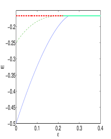
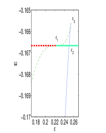
Figure 1: Energy $E$ of the branches considered as a function of $\epsilon$ for a three-site lattice, as provided by Eq. (10) and confirmed by the numeric analysis in Sec. V. Thin solid: stable single pulse; thin dashed: unstable two-pulse (becomes single-pulse-like for $\epsilon>\epsilon_{1}$); thick: unstable (dashed) and stable (solid) portions of the uniform branch. The right panel is a blowup of the left one, and clearly illustrates the relevant critical points.

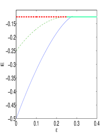
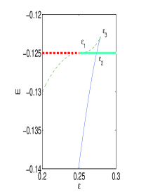
Figure 2: Energy $E$ of the solution branches considered as a function of $\epsilon$ for a four-site lattice, as resulting from the numeric analysis in Sec. V. The line styles and colors have the same meaning as in Fig. 1. The right panel is a blowup of the left one, and clearly illustrate the relevant critical points.

V Numerical techniques and results

A numerical study of the single- and two-pulse solution can be efficiently performed by means of Keller’s pseudo-arclength continuation method keller . This allows us to trace the relevant branches of solutions past fold points. Given a solution $({v_{n}}^{(0)},\epsilon^{(0)})$ of the equation $G({v_{n}};\epsilon)=0$ and a ‘direction’ vector $({{\bar{v}}_{n}}^{(0)},{\bar{\epsilon}}^{(0)})$, one can derive $({v_{n}^{(1)}},\epsilon^{(1)})$ by solving the system of equations

$$\begin{array}[]{c}G_{1}\equiv G({v_{n}^{(1)}},\epsilon^{(1)})=0,\\ \\ ({v_{n}^{(1)}}-{v_{n}^{(0)}})*{\bar{v}}_{n}^{(0)}+(\epsilon^{(1)}-\epsilon^{(0)}){\bar{\epsilon}}^{(0)}-\Delta s=0,\end{array}$$ (11)

where $\Delta s$ is a pre-selected arclength parameter (we typically used $\Delta s=0.001$). The parenthetic superscript denotes the iteration step index. Subsequently, one can use Newton’s method to solve the system in equation  (11). The next (normalized) ‘direction’ vector $({\bar{v}}_{n}^{(1)},{\bar{\epsilon}}^{(1)})$, is then computed by solving

$$\left(\begin{array}[]{cc}\frac{\partial}{\partial v_{n}}G_{1}&\frac{\partial}{\partial\epsilon}G_{1}\\ {\bar{v}}_{n}^{(0)}&{\bar{\epsilon}}^{(0)}\end{array}\right)\left(\begin{array}[]{c}{\bar{v}}_{n}^{(1)}\\ {\bar{\epsilon}}^{(1)}\end{array}\right)=\left(\begin{array}[]{c}0\\ 1\end{array}\right),$$ (12)

and the process is then iterated. In this setting, there is a natural starting point of this iteration process at $\epsilon=0$, where the equation (5) becomes algebraic. In that limit, the “single pulse” branch is given by $v_{n}=\delta_{n,n_{0}}$, with support over the site $n_{0}$, and the “two-site” pulse by $v_{n}=(\delta_{n,n_{0}}+\delta_{n,n_{0}+1})/\sqrt{2}$. These branches are initialized with the above exact profile in this anti-continuum limit of $\epsilon=0$, and subsequent continuation of the solutions allows their path-following, as the parameter $\epsilon$ is varied. For each step, once these solutions are obtained, their numerical linear stability is performed by using:

$$u_{n}=e^{i\Lambda t}\left[v_{n}+\delta\left(a_{n}e^{-\lambda t}+b_{n}e^{\lambda^{\ast}t}\right)\right],$$ (13)

where $\delta$ is a formal linearization parameter. This results into a linear (matrix) eigenvalue problem for $(\lambda,\{a_{n},b_{n}^{\star}\})$ that we also solve.

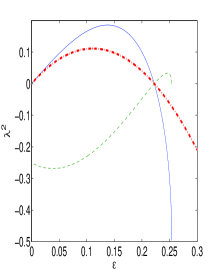
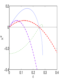
Figure 3: Squared eigenvalues $\lambda^{2}$ of the $M=3$ (left) and $M=4$ (right) case, as a function of $\epsilon$. Thick (thin) lines refer to the uniform (two-site pulse) branch. Note that for $M=4$ an additional eigenvalue for the uniform state exists and is shown.

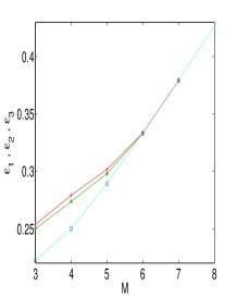
Figure 4: Location of the critical points discussed in the text, with increasing lattice size $M$. Circles, stars and plus symbols denote $\epsilon_{1}$, $\epsilon_{2}$ and $\epsilon_{3}$, respectively. The line joining the circles shows the theoretical prediction of Eq. (6). The other lines are mere guides to the eye.

The analytical description obtained above for the $M=3$ case is confirmed by our numerical results, and remains qualitatively the same for $M=4$ and $M=5$. The situation for $M=4$ is illustrated in figure 2 and 3. Figure 2 shows the behaviour of the energy as a function of $\epsilon$. As in Fig. 1, the right panel is a zoom into the most interesting region. Solid lines denote stable branches, whereas dashed lines denote unstable branches, as specified in the captions. The evident analogies between the three- and four-site lattices (also present for $M=5$, not shown) can be summarized as follows. At the critical point where the modulational instability arises, $\epsilon=\epsilon_{1}(M)$, the two-pulse branch “collides” with the uniform branch, and “emerges” from it as a (higher-energy) single site-branch. This eventually collides with the low-energy single-site branch at $\epsilon=\epsilon_{3}(M)$. The latter originates from the single-pulse solution at $\epsilon=0$, and is the ground state of the system until it crosses the uniform branch at $\epsilon=\epsilon_{2}(M)<\epsilon_{3}(M)$. Note however that this crossing is not a collision in the bifurcation sense, since the configurations of the two branches remain different at this point. They merely have the same energy for fixed norm.

Also, the collision occurring at $\epsilon_{1}(M)$ appears to be definitely non-standard, from a bifurcation theory point of view. This is not only because of the “tangency” of the two branches at the critical point, but also due to the fact that, contrary to what would be expected from such an apparent transcritical bifurcation, the branches do not exchange their stability, but rather the two-pulse branch remains linearly unstable (before, as well as after the collision). Further insight in the non-standard nature of the bifurcation at $\epsilon_{1}(M)$ is gained from Fig. 3, showing, for both $M=3$ and $M=4$, the crucial squared eigenvalues of the two-site and uniform branches, as resulting from our numerical analysis. More specifically, the principal (i.e., maximal) eigenvalue responsible for the instability of the uniform mode turns out to be a double eigenvalue. This double eigenvalue approaches $\lambda=0$, as $\epsilon\rightarrow\epsilon_{1}$ (recall that stabilization implies that this real eigenvalue pair should become imaginary as $\epsilon$ crosses $\epsilon_{1}$, hence its square should change sign). For the two-site branch, an imaginary eigenvalue (for $\epsilon<\epsilon_{1}$, shown by green line in the figures) tends to zero (and becomes real for $\epsilon>\epsilon_{1}$). However, in order for the multiplicity to be preserved (given the double eigenvalue of the uniform state), an additional eigenvalue should cross zero at this critical point (this time, coming from the real side, namely the blue line in Fig. 3). As a result, along the former eigendirection, indeed there is a transcritical exchange of stability, however, the latter eigendirection enforces an additional change of stability for the two-site branch. This results in a novel and non-standard scenario that we call the “double transcritical” bifurcation resulting in one of the branches being unstable before and unstable after the critical point.

Concerning the ground-state properties of such small-size lattices, the above analysis and numerics confirm an important feature made visible by the analytical study of the case $M=3$, that is the presence of a critical value of $\epsilon$ where the inversion in the nature of the ground state takes place. This feature, in fact, does not always occur at the critical point for the modulational instability of the uniform state, $\epsilon_{1}$, but rather at the crossing point $\epsilon_{2}$ previously discussed. That is to say, there is an interval $I_{1}=[\epsilon_{1},\epsilon_{2}]$ where the ground state is localized despite that the uniform state is modulationally stable. Likewise, there is an interval $I_{2}=[\epsilon_{2},\epsilon_{3}]$ where the ground state is uniform, and the single-pulse state is an excited (i.e., higher energy for the same norm) stable state. A further feature worth emphasizing is that the latter terminates at a finite value, $\epsilon=\epsilon_{3}$, due to its collision with the high-energy single-pulse branch discussed above. This is perhaps contrary to the common intuition based on the infinite lattice miw , where the single-pulse branch exists up to the continuum limit, $\epsilon\to\infty$.

Finally, Fig. 4 shows the location of the critical points $\epsilon_{1}$, $\epsilon_{2}$ and $\epsilon_{3}$ with increasing lattice sizes $M$. This indicates how to reconcile the above picture with the infinite lattice limit kapitula , where the uniform state is always modulationally unstable, the single-pulse state is always the ground state, and the latter collides with the two-pulse branch only at $\epsilon\rightarrow\infty$. More specifically, Fig. 4 shows that the picture offered above with the relevant regimes persists for 3-, 4- and 5-site lattices, while for lattices with 6 or more sites the three critical points marking the boundaries of intervals $I_{1}$ and $I_{2}$ collapse to the single value $\epsilon_{1}(M)$ described by Eq. (6). That is to say, for $M\geq 6$ the two intervals shrink to a single point, and the change in the nature of the ground state occurs at the critical point for the modulational instability of the uniform state. Furthermore, for sufficiently large $M$’s, the latter is basically linear in the lattice size $\epsilon_{1}(M)\approx M/2\pi$, so that the above discussed picture is recovered in the thermodynamic limit $M\to\infty$.

VI Conclusions

We have illustrated that dynamical lattices (and, in particular, small ones) still harbor a variety of surprises. They can host previously unraveled bifurcations (such as the “double transcritical” one elucidated above); they may feature ground state inversions, as well as coexistence of stability between uniform and localized states. They may even be unable to sustain localized solutions for sufficiently strong tunneling. All these numerically observed traits can also be captured analytically.

Among the various features we have discussed in section V, the inversion effect characterizing the ground state of small lattices appears to be particularly interesting. For $M=\,3,4,5$ both the uniform state and the single-pulse state are stable solutions of the model within the interval $\epsilon_{1}\leq\epsilon\leq\epsilon_{3}$. Such an interval is absent for $M\geq 6$. The unexpected feature that we have evidenced is that at the intermediate value $\epsilon_{2}$ of such an interval a change in the nature of the ground state between the uniform and the single-pulse state takes place. This inversion is driven by the parameter $\epsilon$. An interesting consequence of this feature is that, at least in principle, by adiabatically decreasing $\epsilon$ across $\epsilon_{2}$ the system can remain in the uniform state without decaying in the proper (single-pulse) ground state. A similar effect can be enacted when adiabatically increasing $\epsilon$ over $\epsilon_{2}$. In this case the single-pulse state (the ground state for $\epsilon<\epsilon_{2}$) survives for $\epsilon>\epsilon_{2}$ once more leaving the system in an excited state.

As discussed above, current experimental technology furnishing two-site lattices markus2 makes forthcoming the realization of $M>2$ small lattices. Given the experimental tractability of both optical waveguide arrays reviews1 and BECs in optical lattices reviews2 , the features we have shown to distinguish few-site lattices should have directly measurable implications in nonlinear optics, as well as soft condensed matter physics. They also generate further intriguing questions, such as e.g. the origin of the “criticality” of the 6-site lattice which are particularly worthwhile to address in future studies.

Acknowledgments. One of the authors (PB) acknowledges a grant from Lagrange project-CRT Foundation and the hospitality of the Ultra Cold Atoms group at the University of Otago. PGK gratefully acknowledges the support of NSF through the grants DMS-0204585, DMS-CAREER and DMS-0505663.

References

- (1) S. Aubry, Physica D 103, 201, (1997); S. Flach and C.R. Willis, Phys. Rep. 295 181 (1998); D. Hennig and G. Tsironis, Phys. Rep. 307, 333 (1999); P. G. Kevrekidis, K.O. Rasmussen, and A. R. Bishop, Int. J. Mod. Phys. B 15, 2833 (2001).
- (2) D. N. Christodoulides, F. Lederer and Y. Silberberg, Nature 424, 817 (2003); Yu. S. Kivshar and G. P. Agrawal, Optical Solitons: From Fibers to Photonic Crystals, Academic Press (San Diego, 2003).
- (3) R. Franzosi, V. Penna, and R. Zecchina, Int. J. Mod. Phys. B 14, 943 (2000); A. Trombettoni, A. Smerzi, Phys. Rev. Lett. 86, 2353 (2001); A. Polkovnikov, S. Sachdev, and S. M. Girvin, Phys. Rev. A 66, 053607 (2002); P. G. Kevrekidis and D.J. Frantzeskakis, Mod. Phys. Lett. B 18, 173 (2004). V. V. Konotop and V. A. Brazhnyi, Mod. Phys. Lett. B 18 627, (2004).
- (4) M. Peyrard, Nonlinearity 17, R1 (2004).
- (5) N. K. Efremidis, S. Sears, and D. N. Christodoulides, Phys. Rev. E 66, 046602 (2002); A. A. Sukhorukov, Y. S. Kivshar, H. S. Eisenberg, and Y. Silberberg, IEEE J. Quantum Elect. 39, 31 (2003).
- (6) J. W. Fleischer, T. Carmon, M. Segev, N. K. Efremidis, and D. N. Christodoulides, Phys. Rev. Lett. 90 023902 (2003); H. Martin, E. D. Eugenieva, Z. Chen, and D. N. Christodoulides Phys. Rev. Lett. 92 123902 (2004); J. Yang, A. Bezryadina, I. Makasyuk, and Z. Chen, Opt. Lett. 29, 1662 (2004); Z. Chen, H. Martin, E. D. Eugenieva, J. Xu, and A. Bezryadina Phys. Rev. Lett. 92 143902 (2004), Z. Chen, J. Yang, A. Bezryadina, and I. Makasyuk, Opt. Lett. 29 1656 (2004).
- (7) S. Burger, K. Bongs, S. Dettmer, W. Ertmer, K. Sengstock, A. Sanpera, G. V. Shlyapnikov, and M. Lewenstein, Phys. Rev. Lett. 83, 5198 (1999); J. Denschlag et al., Science 287, 97 (2000); B. P. Anderson, P. C. Haljan, C. A. Regal, D. L. Feder, L. A. Collins, C. W. Clark, and E. A. Cornell, Phys. Rev. Lett. 86, 2926 (2001); K. E. Strecker, G. B. Partridge, A. G. Truscott, R. G. Hulet, Nature 417, 150 (2002); L. Khaykovich, F. Schreck, G. Ferrari, T. Bourdel, J. Cubizolles, L. D. Carr, Y. Castin, C. Salomon, Science 296, 1290 (2002); B. Eiermann, Th. Anker, M. Albiez, M. Taglieber, P. Treutlein, K.-P. Marzlin, and M. K. Oberthaler, Phys. Rev. Lett. 92, 230401 (2004); R. K. Lee, E. A. Ostrovskaya, Y. S. Kivshar, and Yinchieh Lai Phys. Rev. A 72, 033607 (2005).
- (8) J. C. Eilbeck, P. S. Lomdahl, and A. C. Scott, Physica D 16, 318 (1985).
- (9) R. K. Jackson and M.I. Weinstein, J. Stat. Phys. 116, 881 (2004); K. W. Mahmud, J. N. Kutz, and W. P. Reinhardt, Phys. Rev. A 66, 063607 (2002).
- (10) M. Johansson, J. Phys. A 37, 2201 (2004).
- (11) R. Franzosi and V. Penna, Phys. Rev. E 67, 046227 (2003), G. Chong, W. Hai, and Q. Xie, Phys. Rev. E 70, 036213 (2004), G. Chong, W. Hai, and Q. Xie, ibid. 71, 016202 (2005).
- (12) C. L. Pando, Phys. Lett. A 309, 68 (2003), C. L. Pando L. and E. J. Doedel, Phys. Rev. E 71, 056201 (2005)
- (13) P. G. Kevrekidis, Zhigang Chen, B. A. Malomed, D. J. Frantzeskakis, M. I. Weinstein, Phys. Lett. A 340, 275 (2005); C. Cambournac, T. Sylvestre, H. Maillotte, B. Vanderlinden, P. Kockaert, Ph. Emplit, and M. Haelterman, Phys. Rev. Lett. 89, 083901 (2002).
- (14) Th. Anker, M. Albiez, R. Gati, S. Hunsmann, B. Eiermann, A. Trombettoni, and M. K. Oberthaler, Phys. Rev. Lett. 94, 020403 (2005).
- (15) M. Albiez, R. Gati, J. Fölling, S. Hunsmann, M. Cristiani, M. K. Oberthaler, Phys. Rev. Lett. 95, 010402 (2005).
- (16) P. B. Blakie and C. W. Clark, J. Phys. B 37 1391 (2004); L. Santos, M. A. Baranov, J. I. Cirac, H.-U. Everts, H. Fehrmann, and M. Lewenstein, Phys. Rev. Lett. 93, 030601 (2004); L. Sanchez-Palencia and L. Santos, Phys. Rev. A 72 053607 (2005);
- (17) L. Amico, A. Osterloh, and F. Cataliotti, Phys. Rev. Lett. 95, 063201 (2005).
- (18) L. Amico, and V. Penna, Phys. Rev. Lett. 80, 2189 (1998),
- (19) P. Buonsante, V. Penna, and A. Vezzani, Phys. Rev. A 71, 023610 (2005);
- (20) M.W. Jack and M. Yamashita, Phys. Rev. A 72 043602 (2005);
- (21) M.P.A. Fisher, P.B. Weichman, G. Grinstein and D.S. Fisher, Phys. Rev. B 40, 546 (1989).
- (22) D. Jaksch, C. Bruder, J.I. Cirac, C.W. Gardiner and P. Zoller Phys. Rev. Lett. 81, 3108 (1998).
- (23) M. Theis, G. Thalhammer, K. Winkler, M. Hellwig, G. Ruff, R. Grimm and J. H. Denschlag, Phys. Rev. Lett. 93, 123001 (2004).
- (24) Notice that Hamiltonian (2) differs from those in Refs. ampe ; praBPV by a term that is proportional to the total population, . Since is conserved, this additional term affects the dynamics of only through a site-independent phase factor.
- (25) see e.g. E. Doedel Numerical analysis of bifurcation problems (Hamburg 1997) available at: ftp://ftp.cs.concordia.ca/pub/doedel/doc/
- (26) M.I. Weinstein, Nonlinearity 12, 673 (1999).
- (27) T. Kapitula and P. G. Kevrekidis, Nonlinearity 18, 2491 (2005).