The origin of phase in the interference of Bose-Einstein condensates

Abstract

We consider the interference of two overlapping ideal Bose-Einstein condensates. The usual description of this phenomenon involves the introduction of a so-called condensate wave functions having a definite phase. We investigate the origin of this phase and the theoretical basis of treating interference. It is possible to construct a phase state, for which the particle number is uncertain, but phase is known. However, how one would prepare such a state before an experiment is not obvious. We show that a phase can also arise from experiments using condensates in Fock states, that is, having known particle numbers. Analysis of measurements in such states also gives us a prescription for preparing phase states. The connection of this procedure to questions of “spontaneously broken gauge symmetry” and to “hidden variables” is mentioned.

I INTRODUCTION

One of the most impressive experiments using trapped Bose gases is the interference experiment of Ketterle and co-workers.Ketterle Two condensates are are separately prepared and allowed to overlap. An interference pattern then arises showing the remarkable quantum coherence of the condensates. There have been other interesting condensate interference experiments as well.Int2 ^-Hall If one assumes that the separated clouds initially have a definite phase relation, then the experiments are well-described by straight-forward theory.Nara However, questions immediately arise. Do separately prepared condensates have a phase relation?A-3 The preparation of the sample certainly did not involve the establishment of a state with known phase. More likely the particle number in each cloud would have, or could have, been initially known ahead of time. Nevertheless an interference pattern emerges with some well-established phase. So how is this possible? The question was answered in several theoretical papers showing how a phase appears even when the two clouds are prepared in Fock states, that is, states with sharply known particle numbers.JH ^-PS In this paper we revisit the question and present a derivation of this result. This result is quite satisfying, since it in a sense justifies the usual simple assumption of the interferring coherent systems having a well-defined, but completely unknown, initial phase relationship.

In order to discuss the properties of condensates and superfluids one usually introduces theoretically a so-called “order parameter” or “condensate wave function” defined as $\left\langle\hat{\psi}(\mathbf{r})\right\rangle$ where $\hat{\psi}(\mathbf{r})$ is an operator destroying a particle at position $\mathbf{r.}$ The resulting quantity has a magnitude equal to the square root of the condensate density and also a phase. Obviously the state in which $\left\langle\hat{\psi}(\mathbf{r})\right\rangle$ is non-zero cannot have a fixed particle number. With one of these wave functions for each condensate, it is straightforward to discuss interference of the two, since each one has its own phase, and an interference pattern arises with a relative phase equal to the difference between the individual phases. In essence one has described each condensate by a single-particle wave function so that interference is no more than the overlap and interference of two classical waves. However, one can ask how this single-particle wave function might have arisen. Indeed its existence involves the question of “spontaneously broken gauge symmetry”A-2 ^-Leggett , the necessity of which has been brought into question in recent years.LS ^-Johnston

Suppose we consider a condensate described by a wave function $e^{i(\mathbf{k\cdot r}+\phi)}.$ One might describe the direction specified by the angle $\phi$ by a “spin” in a two-dimensional plane. How do we prepare such a state? What is it that picks out the direction of this pseudo-spin from the all the degenerate possible directions? There is an analogy with ferromagnetism, where there is symmetry in the possible degenerate three-dimensional directions of the magnetization. Somehow, say, because of a small external field, a particuliar direction is space is picked out for the magnetization. In a similar way the phase angle is picked out. One can suppose in the ferromagnetism case that, in actual practice, there is always some small field to pick out a preferred direction, so that the symmetry is broken. However, the local field that is used theoretically to pick a phase direction does not exist in nature. Indeed one would have to prepare a state that does not have a fixed particle number. The treatment of phase (actually relative phase) in Sec. IV, and the spontaneous appearance of a relative phase under the effect of measurement of particle position in Fock states, avoids violating particle conservation and does not require use of any symmetry-breaking field and so helps in this regard.

A closely related feature of the discussion is the idea that the phase emerging from successive measurements of particle position starting with a Fock state is somewhat like the emergence of a “hidden” or “additional” variable in quantum mechanics.FLHidden ^,Bell-0 ^,FL-1 Was the phase there before the experiment started, or did the experiment itself cause it to take on its final value? Hidden variables can be invoked to specify non-commuting variables. In standard quantum mechanics, particle number and relative phase can be considered conjugate variables; the knowledge of one excludes that of the other. As we measure particle position we will see that the knowledge of the particle number becomes less certain while the uncertainty of relative phase decreases.

In the next sections we first discuss the kind of state that has a known phase. Obviously with this state the interference pattern emerges with just the prepared phase. Among these states are are the coherent states of Glauber.G These can either have particle number completely unknown or have the total number of particles in two clouds known (in which case they are called “phase states”), although the number in each cloud is still unknown. We then derive the interference pattern starting with Fock states and see the emergence of a relative phase even though no phase was present at the beginning of the experiment (or was at least “hidden”). We even find a way to prepare a state that has a known relative phase. The controversal theoretical constructs are seen to be unnecessary.

II SIMPLE VIEW OF AN INTERFERENCE PATTERN

A gas (or liquid) undergoing Bose-Einstein condensation (BEC) is often described by a classical field known as an “order parameter” or “condensate wave function.” Such a quantity can arise in several ways. Suppose that $\hat{\psi}(\mathbf{r})$ represents a second-quantized operator destroying a boson at position $\mathbf{r}$. Then the one-particle density matrix is defined as $\rho(\mathbf{r},\mathbf{r}^{\prime})=\left\langle\hat{\psi}^{\dagger}(\mathbf{r})\hat{\psi}(\mathbf{r})\right\rangle.$ Penrose and OnsagerPO showed that a criterion for a Bose condensate or “off-diagonal long-range order” is that the density matrix have the form

$$\rho(\mathbf{r},\mathbf{r}^{\prime})=\psi^{*}(\mathbf{r})\psi(\mathbf{r}^{\prime})+f(\mathbf{r},\mathbf{r}^{\prime})$$ (1)

where $f(\mathbf{r},\mathbf{r}^{\prime})$ vanishes when $\left|\mathbf{r}-\mathbf{r}^{\prime}\right|\rightarrow\infty$ . The function $\psi(\mathbf{r})$ is the condensate wave function. One often assumes the system in a state such that the destruction operator itself has a non-zero average:

$$\left\langle\hat{\psi}(\mathbf{r})\right\rangle=\psi(\mathbf{r})=\sqrt{n_{0}(\mathbf{r})}e^{i\phi(\mathbf{r})}$$ (2)

where $n_{0}$ is the condensate density and $\phi$ its phase. Such a state is said to have “spontaneously broken gauge symmetry” because a particular phase (out of many possible degenerate phase states) has been chosen.A-2 ^- Johnston The Gross-Pitaevskii equation is a non-linear Schrodinger equation for $\psi(\mathbf{r}),$ which has been used extensively, with remarkable success, to describe interacting trapped BEC gases within mean-field approximation.Stringari

In describing the interference pattern of the experiment of Ref. Ketterle, one has to consider the overlap of Bose clouds released from harmonic oscillator traps.Nara This leads to some interesting features such as fringes whose separation changes with time. In our analysis here we will consider only plane waves and ignore any time evolution. Thus suppose we have an order parameter that involves two condensate clouds, having condensate densities $n_{a}$ and $n_{b}$ in momentum states $\mathbf{k}_{a}$ and $\mathbf{k}_{b}.$ This dual order parameter has the form

$$\psi(\mathbf{r})=\sqrt{n_{a}}e^{i\mathbf{k}_{a}\mathbf{r}}e^{i\phi_{a}}+\sqrt{n_{b}}e^{i\mathbf{k}_{b}\mathbf{r}}e^{i\phi_{b}}.$$ (3)

The density of the combined system is then

$$n(\mathbf{r})=\left|\sqrt{n_{a}}e^{i\mathbf{k}_{a}\mathbf{r}}e^{i\phi_{a}}+\sqrt{n_{b}}e^{i\mathbf{k}_{b}\mathbf{r}}e^{i\phi_{b}}\right|^{2}=n\left(1+x\cos(\mathbf{k\cdot r}+\phi)\right)$$ (4)

where $n=n_{a}+n_{b},$ $\mathbf{k}=\mathbf{k}_{a}-\mathbf{k}_{b}$, $\phi=\phi_{b}-\phi_{a},$ and $x=2\sqrt{n_{a}n_{b}}/n.$ We have an interference pattern with relative phase $\mathbf{k\cdot r}+\phi.$ The phase shift $\phi$ is measureable although the individual phases $\phi_{a}$ and $\phi_{b}$ are not.

This analysis is simple, but it requires the preparation of the system in a state with known individual phases. How do we do that? What is the nature of such a state? Clearly the expectation value of Eq. (2) cannot be in a state of definite particle number or the expectation value would vanish. Next we investigate this question more deeply.

III PHASE STATES

As noted by JohnstonJohnston in this journal, the coherent states introduced by GlauberG for photons are appropriate for superfluids. These well-know states have been reviewed in this journal on occasion,coherent and appear in textsCTDL as well. They are also called “classical states” and are the minimum uncertainty states of the harmonic oscillator.CTDL Here we do not use them in full generality, but rather use a subset of them known as “phase states.” (Those wishing to see the full treatment of coherent states in a treatment of a condensate wave function are referred to Appendix A.) Phase states describe two condensates (in states $\mathbf{k}_{a}$ and $\mathbf{k}_{b}$) with variable particle numbers, $N_{a},$ $N_{b}$ (both macroscopic), but fixed total number $N=N_{a}+N_{b}.$ No other momentum states are occupied. If particle creation operators $a^{\dagger}$ and $b^{\dagger}$ (obeying Bose commutation relations) for the two states act on the vacuum to put particles into these two states, then we define the (properly normalized) state as

$$\left|\alpha_{a}\alpha_{b};N\right\rangle = \frac{1}{\sqrt{g^{N}}}\sum_{N_{a}=0}^{N}\sqrt{\frac{N!}{N_{a}!\left(N-N_{a}\right)!}}\alpha_{a}^{N_{a}}\alpha_{b}^{N-N_{a}}\left|N_{a},N-N_{a}\right\rangle$$ (5)

$$= \frac{1}{\sqrt{g^{N}}}\sum_{N_{a}}\frac{\sqrt{N!}}{N_{a}!\left(N-N_{a}\right)!}\left(\alpha_{a}a^{\dagger}\right)^{N_{a}}\left(\alpha_{b}b^{\dagger}\right)^{N-N_{a}}\left|0\right\rangle$$

$$= \sqrt{\frac{1}{g^{N}N!}}\left(\alpha_{a}a^{\dagger}+\alpha_{b}b^{\dagger}\right)^{N}\left|0\right\rangle$$

where we define the quantities $\alpha_{i}$ as complex and separate them into magnitudes $\gamma_{i}$ and phases $\phi_{i}$ according to the notation

$$\alpha_{i}=\gamma_{i}e^{i\phi_{i}}.$$ (6)

Also $g=\sqrt{\gamma_{a}^{2}+\gamma_{b}^{2}}.$ We can easily compute the average number of particles $\bar{N}_{a}$ in this state. Use the first form of Eq. (5) to give

$$a\left|\alpha_{a}\alpha_{b};N\right\rangle = \frac{1}{\sqrt{g^{N}}}\sum_{N_{a}}\sqrt{\frac{N!}{N_{a}!\left(N-N_{a}\right)!}}\alpha_{a}^{N_{a}}\alpha_{b}^{N-N_{a}}\sqrt{N_{a}}\left|N_{a}-1,N-N_{a}\right\rangle$$ (7)

$$= \alpha_{a}\frac{\sqrt{N}}{\sqrt{g^{N}}}\sum_{N_{a}^{\prime}}\sqrt{\frac{(N-1)!}{N_{a}^{\prime}!\left(N-1-N_{a}^{\prime}\right)!}}\alpha_{a}^{N_{a}^{\prime}}\alpha_{b}^{N-1-N_{a}^{\prime}}\left|N_{a}^{\prime},N-N_{a}\right\rangle$$

$$= \alpha_{a}\sqrt{\frac{N}{g}}\left|\alpha_{a}\alpha_{b};N-1\right\rangle$$

where we have taken $N_{a}^{\prime}=N_{a}-1.$ Thus

$$\bar{N}_{a}=\left\langle\alpha_{a}\alpha_{b};N\right|a^{\dagger}a\left|\alpha_{a}\alpha_{b};N\right\rangle=\gamma_{a}^{2}\frac{N}{\gamma_{a}^{2}+\gamma_{b}^{2}}$$ (8)

Similarly we get $\bar{N}_{b}=\gamma_{b}^{2}N/(\gamma_{a}^{2}+\gamma_{b}^{2})$ so that $\gamma_{i}=\left|\alpha_{i}\right|=\sqrt{\bar{N}_{i}}$ and $g=N_{a}+N_{b}=N.$

The fact that $N$ is known in our phase state does not affect the results for interference patterns, which depend just on relative phase. Indeed such states have been used on many occasions to discuss the interference of two condensates.CD ^,HB ^,PS ^,KS Our state can be used to discuss the how relative phase can be conjugate to particle number. Write it in a form that makes the phases explicit:

$$\left|\alpha_{a}\alpha_{b};N\right\rangle=\sqrt{\frac{N!}{g^{N}}}\sum_{\left(N_{a}+N_{b}=N\right)}\frac{\gamma_{a}^{N_{a}}\gamma_{b}^{N_{b}}e^{iN_{a}\phi_{a}}e^{iN_{b}\phi_{b}}}{\sqrt{N_{a}!N_{b}!}}\left|N_{a},N_{b}\right\rangle$$ (9)

Now change the phases to relative phase $\phi=\phi_{b}-\phi_{a}$ and total phase $\Phi=(1/2)(\phi_{b}+\phi_{a})$ and then take the derivative with respect to $\phi:$

$$-2i\frac{\partial}{\partial\phi}\left|\alpha_{a}\alpha_{b};N\right\rangle = \sqrt{\frac{N!}{g^{N}}}\sum_{\left(N_{a}+N_{b}=N\right)}(N_{a}-N_{b})\frac{\gamma_{a}^{N_{a}}\gamma_{b}^{N_{b}}e^{iN_{a}(\Phi+\phi/2)}e^{iN_{b}(\Phi-\phi/2)}}{\sqrt{N_{a}!N_{b}!}}\left|N_{a},N_{b}\right\rangle$$ (10)

$$= \left(a^{\dagger}a-b^{\dagger}b\right)\left|\alpha_{a}\alpha_{b};N\right\rangle$$

The phase derivative operator gives the same result as the number difference operator so that $\phi$ and $(N_{a}-N_{b})$ are conjugate variables.Leggett ^,KS Note that the total phase appears only as an external factor $\exp\left[iN\Phi\right]$ and so has no physical significance. Thus the individual phases have no physical significance; only the relative phase $\phi$ is a meaningful quantity.

In order to emphasize this last point and put the phase state in a more compact form to treat interference we rename it and rewrite it as

$$\left|\phi,N\right\rangle=\frac{1}{\sqrt{g^{N}N!}}(a^{\dagger}+\gamma e^{i\phi}b^{\dagger})^{N}\left|0\right\rangle=\frac{1}{\sqrt{g^{N}}}\sum_{n=1}^{N}\sqrt{\frac{N!}{n!(N-n)!}}(\gamma e^{i\phi})^{N-n}\left|n,N-n\right\rangle$$ (11)

where now $\gamma=\sqrt{\bar{N}_{a}/\bar{N}_{b}}$ and $\phi$ is the relative phase. Also now $g=(1+\gamma^{2}).$ We have simply dropped a meaningless factor of unit magnitude.

Since we have just two occupied states, the terms in Eq. (47) not referring to states $k_{a}$ and $k_{b}$ never contribute and we can more simply write

$$\hat{\psi}(\mathbf{r})\rightarrow c_{\mathbf{r}}\equiv\sqrt{\frac{1}{V}}\left(e^{i\mathbf{k}_{a}\cdot\mathbf{r}}a+e^{i\mathbf{k}_{b}\cdot\mathbf{r}}b\right)\mathbf{.}$$ (12)

We can also make this more compact by writing

$$c_{\mathbf{r}}=\sqrt{\frac{1}{V}}\left(a+e^{i\mathbf{k}\cdot\mathbf{r}}b\right)$$ (13)

with $\mathbf{k}=\mathbf{k}_{b}-\mathbf{k}_{a}.$ The quantity extracted out $e^{i\mathbf{k}_{a}\cdot\mathbf{r}}$ can again be dropped as a meaningless unit-magnitude factor. We want to consider how $c_{\mathbf{r}}$ acts on the phase state. We have

$$c_{\mathbf{r}}\left|\phi,N\right\rangle = \frac{1}{\sqrt{g^{N}V}}\sum_{n=1}^{N}\sqrt{\frac{N!}{n!(N-n)!}}(\gamma e^{i\phi})^{N-n}$$ (15)

$$\times\left(\sqrt{n}\left|n-1,N-n\right\rangle+e^{i\mathbf{k}\cdot\mathbf{r}}\sqrt{N-n}\left|n,N-n-1\right\rangle\right)$$

By changing variables in the first state to $n^{\prime}=n-1$ we can put both terms in the same form so

$$c_{\mathbf{r}}\left|\phi,N\right\rangle=A(\mathbf{r,}\phi)\left|\phi,N-1\right\rangle$$ (16)

where

$$A(\mathbf{r,}\phi)=\sqrt{\frac{N}{gV}}\left(1+\gamma e^{i\phi}e^{i\mathbf{k}\cdot\mathbf{r}}\right)$$ (17)

We can now easily compute the condensate wave function as

$$\left\langle\phi,N\right|\hat{\psi}(\mathbf{r})\left|\phi,N\right\rangle=\left\langle\phi,N\right|c_{\mathbf{r}}\left|\phi,N\right\rangle=A(\mathbf{r,}\phi)$$ (18)

If for the moment we put back the previously neglected leading phase factors we have

$$\left\langle\phi,N\right|\hat{\psi}(\mathbf{r})\left|\phi,N\right\rangle=\sqrt{\bar{n}_{a}}e^{i\mathbf{k}_{a}\cdot\mathbf{r}}e^{i\phi_{a}}+\sqrt{\bar{n}_{b}}e^{i\mathbf{k}_{b}\cdot\mathbf{r}}e^{i\phi_{b}}$$ (19)

which has just the same form as Eq. (3), with average densities in place of precise densities and well-defined individual phases. However the individual phases are not measurable—only the relative phase is. Indeed the average density follows immediately as

$$\left\langle\phi,N\right|\hat{\psi}^{\dagger}(\mathbf{r})\hat{\psi}(\mathbf{r})\left|\phi,N\right\rangle=\left\langle\phi,N\right|c_{\mathbf{r}}^{\dagger}c_{\mathbf{r}}\left|\phi,N\right\rangle=\left|A(\mathbf{r},\phi)\right|^{2}=\bar{n}\left(1+\bar{x}\cos(\mathbf{k\cdot r}+\phi)\right)$$ (20)

just like Eq. (4) where now $\bar{n}$ and $\bar{x}$ have obvious definitions in terms of averages. Thus a phase state provides a rigorous background for discussion of condensate wave functions and for the simplified form of treating interference between the two condensates. How we might actually prepare one before the experiment is a separate difficult question, which we treat below.

We will find it useful and necessary in the next section to consider more general cases in which we make measurements of many particle positions essentially simultaneously. This allows interference fringes to emerge where they would otherwise not occur. For our phase state such calculations are straightforward and add no additional information since the the multiparticle densities all factor in the phase states. For example, consider the expectation value of

$$\hat{\psi}^{\dagger}(\mathbf{r}_{2})\hat{\psi}(\mathbf{r}_{2})\hat{\psi}^{\dagger}(\mathbf{r}_{1})\hat{\psi}(\mathbf{r}_{1})=c_{\mathbf{r}_{2}}^{\dagger}c_{\mathbf{r}_{2}}c_{\mathbf{r}_{1}}^{\dagger}c_{\mathbf{r}_{1}}\approx c_{\mathbf{r}_{2}}^{\dagger}c_{\mathbf{r}_{1}}^{\dagger}c_{\mathbf{r}_{2}}c_{\mathbf{r}_{1}}.$$ (21)

Of course, $c_{\mathbf{r}_{2}}$ and $c_{\mathbf{r}_{1}}^{\dagger}$ don’t commute, but in the approximation shown we are dropping a term of order $N$ compared to one of order $N^{2}.$ The last form is more convenient to use. By the eigenfunction behavior of the phase state we easily get

$$\left\langle\phi,N\right|\hat{\psi}^{\dagger}(\mathbf{r}_{2})\hat{\psi}(\mathbf{r}_{2})\hat{\psi}^{\dagger}(\mathbf{r}_{1})\hat{\psi}(\mathbf{r}_{1})\left|\phi,N\right\rangle \approx \left\langle\phi,N\right|c_{\mathbf{r}_{2}}^{\dagger}c_{\mathbf{r}_{1}}^{\dagger}c_{\mathbf{r}_{2}}c_{\mathbf{r}_{1}}\left|\phi,N\right\rangle=\left|A(\mathbf{r}_{2})\right|^{2}\left|A(\mathbf{r}_{1})\right|^{2}$$ (22)

$$= \prod_{i=1}^{2}\bar{n}\left(1+\bar{x}\cos(\mathbf{k\cdot r}_{i}+\phi)\right)$$

This result generalizes to

$$\left\langle\phi,N\right|\hat{\psi}^{\dagger}(\mathbf{r}_{m})\hat{\psi}(\mathbf{r}_{m})\cdots\hat{\psi}^{\dagger}(\mathbf{r}_{1})\hat{\psi}(\mathbf{r}_{1})\left|\phi,N\right\rangle \approx \left\langle\phi,N\right|c_{\mathbf{r}_{m}}^{\dagger}\cdots c_{\mathbf{r}_{1}}^{\dagger}c_{\mathbf{r}_{m}}\cdots c_{\mathbf{r}_{1}}\left|\phi,N\right\rangle$$ (23)

$$= \prod_{i=1}^{m}\bar{n}\left(1+\bar{x}\cos(\mathbf{k\cdot r}_{i}+\phi)\right)$$

Considering a state in the form $c_{\mathbf{r}_{m}}\cdots c_{\mathbf{r}_{1}}\left|\Psi\right\rangle$ is useful for interpreting an experiment. Here we can consider our experiment as detecting particle 1 and then 2 shortly thereafter, and so on. After $m$ detections the wave function evolves to a state missing several particles. What is the nature of the state to which it has evolved? In the case of a phase state it is $c_{\mathbf{r}_{m}}\cdots c_{\mathbf{r}_{1}}\left|\phi,N\right\rangle\sim\left|\phi,N-m\right\rangle.$ However, it is more interesting to consider the case of $\left|\Psi\right\rangle$ a Fock state as we do in the next section.

IV INTERFERENCE IN FOCK STATES

It is not evident that experimentalists can prepare a phase state as described above. It would seem more likely that they are working with Fock states, that is, states in which the particles numbers, $N_{a}$ and $N_{b},$ in the two condensates are known rather well. It seems likely, in any case, that one has more chance of initially preparing such a state. However, as several workersJH ^-PS have realized in recent years, and as we will show, that an interference pattern with some phase can still arise in a Fock state. Denoting the state sharp in particle number as $\left|N_{a},N_{b}\right\rangle$ and using the Bose annihilation relation

$$c_{\mathbf{r}}\left|N_{a},N_{b}\right\rangle=\sqrt{\frac{1}{V}}\left(\sqrt{N_{a}}\left|N_{a}-1,N_{b}\right\rangle+e^{i\mathbf{k}\cdot\mathbf{r}}\sqrt{N_{b}}\left|N_{a},N_{b}-1\right\rangle\right)$$ (24)

the one-body density in a Fock state is

$$D_{1}=\left\langle N_{a},N_{b}\right|c_{\mathbf{r}}^{\dagger}c_{\mathbf{r}}\left|N_{a},N_{b}\right\rangle=n$$ (25)

and of course there is no interference. Phase and particle number are conjugates, and the particle number is initially known.

However, if we consider measuring the position of two particles simultaneously, some correlation should arise. We have

$$c_{\mathbf{r}_{2}}c_{\mathbf{r}_{1}}\left|N_{a},N_{b}\right\rangle = \frac{1}{V}\left[\sqrt{N_{a}(N_{a}-1)}\left|N_{a}-2,N_{b}\right\rangle+e^{i\mathbf{k}\cdot\left(\mathbf{r}_{1}+\mathbf{r}_{2}\right)}\sqrt{N_{b}(N_{b}-1)}\left|N_{a},N_{b}-2\right\rangle\right.$$ (26)

$$+\left.\sqrt{N_{a}N_{b}}\left(e^{i\left(\mathbf{k}\cdot\mathbf{r}_{1}\right)}+e^{i\left(\mathbf{k}\cdot\mathbf{r}_{2}\right)}\right)\left|(N_{a}-1)(N_{b}-1)\right\rangle\right]$$

so that the particle number is now slightly less certain. The two-body Fock correlation function is

$$D_{2} = \left\langle N_{a},N_{b}\right|c_{\mathbf{r}_{1}}^{\dagger}c_{\mathbf{r}_{2}}^{\dagger}c_{\mathbf{r}_{2}}c_{\mathbf{r}_{1}}\left|N_{a},N_{b}\right\rangle$$ (27)

$$= \frac{1}{V^{2}}\left[N_{a}(N_{a}-1)+N_{b}(N_{b}-1)+N_{a}N_{b}\left|e^{i\left(\mathbf{k}\cdot\mathbf{r}_{1}\right)}+e^{i\left(\mathbf{k}\cdot\mathbf{r}_{2}\right)}\right|^{2}\right]$$

$$= n^{2}\left[1+x\cos\mathbf{k\cdot}(\mathbf{r}_{1}-\mathbf{r}_{2})\right]$$

For two particles there is indeed a position correlation. As we make more and more measurements the state gets more and more mixed among states with various numbers of particles.

We can rewrite Eq. (27) in a somewhat different and useful way. A simple integration shows that

$$D_{2}=n^{2}\int_{0}^{2\pi}\frac{d\phi}{2\pi}\prod_{i=1}^{2}\left[1+x\cos(\mathbf{k\cdot r}_{i}+\phi)\right].$$ (28)

Compare this with Eq. (22). We have a similar looking result except that we now integrate over all relative phases. Remarkably this result can be extended to higher order correlation functions. Indeed Ref. FLHidden, shows that

$$D_{m}=n^{m}\int_{0}^{2\pi}\frac{d\phi}{2\pi}\prod_{i=1}^{m}\left[1+x\cos(\mathbf{k\cdot r}_{i}+\phi)\right]$$ (29)

where it is assumed that $m<<N$.

In order to derive this result, we invert Eq. (11). Multiply both sides by $e^{-i\phi(N-n)}=e^{-i\phi N_{b}}$ and integrate over $\phi$ to give

$$\left|N_{a},N_{b}\right\rangle=\frac{g^{N/2}}{\gamma^{N_{b}}}\sqrt{\frac{N_{a}!N_{b}!}{N!}}\int_{0}^{2\pi}\frac{d\phi}{2\pi}e^{-i\phi N_{b}}\left|\phi,N\right\rangle$$ (30)

Thus, by Eq. (16), we find

$$c_{\mathbf{r}_{m}}\cdots c_{\mathbf{r}_{1}}\left|N_{a},N_{b}\right\rangle\sim\int_{0}^{2\pi}\frac{d\phi}{2\pi}e^{-i\phi N_{b}}\prod_{i=1}^{m}A(\mathbf{r}_{i},\phi)\left|\phi,N-m\right\rangle$$ (31)

We will return to analyze this interesting state below. First consider the $m$-body Fock correlation function:

$$D_{m} = \left\langle N_{a},N_{b}\right|c_{\mathbf{r}_{m}}^{\dagger}\cdots c_{\mathbf{r}_{1}}^{\dagger}c_{\mathbf{r}_{m}}\cdots c_{\mathbf{r}_{1}}\left|N_{a},N_{b}\right\rangle$$ (32)

$$\sim \int_{0}^{2\pi}\frac{d\phi^{\prime}}{2\pi}\int_{0}^{2\pi}\frac{d\phi}{2\pi}e^{-i\left(\phi-\phi^{\prime}\right)N_{b}}\prod_{i=1}^{m}A^{*}(\mathbf{r}_{i},\phi^{\prime})A(\mathbf{r}_{i},\phi)\left\langle\phi^{\prime},N-m\right|\left|\phi,N-m\right\rangle$$ (33)

Phase states are not actually orthogonal, but for large $N$ they are essentially so as we show in Appendix A, so, if $m\ll N,$ we can write $\left\langle\phi^{\prime},N-m\right|\left|\phi,N-m\right\rangle\sim\delta(\phi-\phi^{\prime})$ and

$$D_{m}\sim\int_{0}^{2\pi}\frac{d\phi}{2\pi}\prod_{i=1}^{m}\left|A(\mathbf{r}_{i},\phi)\right|^{2}$$ (34)

just as we claimed in Eq. (29). We will show how to get this result by direct calculation, as done in Ref. FLHidden, , in Appendix B.

This result Eq. (29) has the form of Eq. (23) but with the unknown phase integrated over. That makes sense in that our initial Fock state did not have a phase defined and can, indeed, itself be expressed as a sum over phase states as in Eq. (30).

Suppose we have started with a Fock state and have made $m-1$ particle measurements and have found particles at positions $\mathbf{R}_{1},\cdots,\mathbf{R}_{m-1}$ and are about to measure the $m$th. Then the probability of finding the $m$th particle at position $\mathbf{r}_{m}$ is

$$P_{m}=n^{m}\int_{0}^{2\pi}\frac{d\phi}{2\pi}g_{m}(\phi)\left[1+x\cos(\mathbf{k\cdot r}_{m}+\phi)\right]$$ (35)

where

$$g_{m}(\phi)=\prod_{i=1}^{m-1}\left[1+x\cos(\mathbf{k\cdot R}_{i}+\phi)\right]$$ (36)

As we show by direct simulation, $g(\phi)$ develops a sharp peak at some a priori unpredictable phase. If one makes measurements from the first to the $m$th particle by this prescription, the peak becomes narrower as one proceeds. Of course, as more measurements are made, the particle number in each condensate becomes less certain (as, for example, in Eq. (26)), so phase can be more sharply defined.

Now look back at Eq. (31). After a fair number $m$ of measurements, the real part of $\prod_{i=1}^{m}A(\mathbf{r}_{i},\phi)$ peaks up sharply at some $\phi$ value, call in $\phi_{0}$. That means that the measurements have converted the Fock wave function into a narrow sum of phase states around $\left|\phi_{0},N-m\right\rangle.$ The more measurements that are made, the better is the definition of the phase state. Measurements in a Fock state provide a way to prepare a phase state. One can understand the MIT experimentsKetterle in this way. The starting state was prepared as two separate condensates, whose particle numbers could have been known; many subsequent particle measurements sharpened the phase to some random value and the final overall observation showed that phase.

V NUMERICAL SIMULATION

We use Eqs. (35) and (36). One choses the initial position $\mathbf{r}_{1}$ randomly, and then the next particle is chosen from the probability distribution $P_{2}$ and so on. We will find that, if $m$ is large enough, $g_{m}$ peaks up at some a priori unpredictable phase angle, $\phi_{0}$ which may fluctuate somewhat as $m$ changes but gradually settles down. Starting a new experiment from the Fock state will lead to a randomly different phase angle. We will consider only the case in which the initial Fock state has $N_{a}=N_{b}=N/2,$ i.e., $x=1.$ It is convenient to Fourier expand $g_{m}.$ That is, we write

$$g_{m}(\phi)=a_{0}+\sum_{q=1}^{\infty}\left[a_{q}\cos q\phi+b_{q}\sin q\phi\right]$$ (37)

In the integration of Eq. (35) only $a_{0},$ $a_{1,}$ and $b_{1}$ will contribute and doing the integrals gives

$$P_{m}(\mathbf{r}_{m})\sim 1+\frac{a_{1}}{2a_{0}}\cos(\mathbf{k\cdot r}_{m})-\frac{b_{1}}{2a_{0}}\sin(\mathbf{k\cdot r}_{m})$$ (38)

If we define $\cos(\phi_{m})\equiv a_{1}/\sqrt{a_{1}^{2}+b_{1}^{2}}$, $\sin(\phi_{m})\equiv b_{1}/\sqrt{a_{1}^{2}+b_{1}^{2}},$ and $A_{m}\equiv\sqrt{a_{1}^{2}+b_{1}^{2}}/2a_{0},$ we can write

$$P_{m}=K[1+A_{m}(\cos\mathbf{k\cdot r}_{m}\cos\phi_{m}-\sin\mathbf{k\cdot r}_{m}\sin\phi_{m})]=K\left(1+A_{m}\cos(\mathbf{k\cdot r}_{m}+\phi_{m})\right).$$ (39)

where $K$ is a normalization factor, and

$$\tan(\phi_{m})=\frac{b_{1}}{a_{1}}.$$ (40)

gives the the value of an angle in the $m$th experiment. Since $P_{m}$ is a probability, we must have $A_{m}<1$ so that $P_{m}$ is always positive. Since $A_{m}$ has that property we can write $A_{m}\equiv\sin(\alpha_{m})$ where $0<\alpha_{m}<\pi$ behaves like a polar angle. Then the emerging phase actually has a space angle designation ($\alpha_{m},\phi_{m}).$ We will find numerically that $A_{m}\rightarrow 1$ rapidly as we make measurements. In that case the probability of Eq. (39) looks just like the density prediction of Eq. (4) and moreover since $g_{m}(\phi)$ is a narrow function peaking at $\phi_{0},$ the phase defined by the Fourier coefficients is the same as that defined by the peak of $g_{m},$ as seen using Eq. (35).

We work in just one dimension. To choose from the probability of Eq. (38), we need to find the cumulative probability $C_{m}(x)=\int_{0}^{x}dx^{\prime}P_{m}(x^{\prime})$ and then solve the equation $R=C_{m}(x)$ for $x,$ where $R$ is a random number uniformly distributed on $0$ to $1.$ We take the box size $L=1$ and choose a $k$ value such that $kL$ is an integer times 2$\pi$ to provide periodic boundary conditions. The normalization of the probability in Eq.(39) is just the factor $K=1/L=1.$

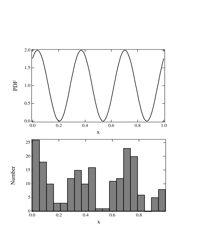
Figure 4: The probability distribution function for position in the interference pattern as calculated and the histogram of this as found in simulated experiments. The phase is found here to be the same as in the other approaches.

Figs. 1 and 2 are plots of $\phi_{m}$ and $A_{m}$ versus iteration number in a particular run of 200 interations; each of these is found from the amplitudes $a_{0},$ $a_{1},$ $b_{1}$ at each iteration. There is no reason why $A_{m}$ should be unity from the outset. However, $A_{m}$ does always proceed to unity after a small number of iterations. The result is that $\phi_{m}$ approaches some sharply-defined random phase angle as predicted. Of course, for small $m$ the fluctuations are relatively large and settle down only after many measurements. This corresponds to an initially wide distribution, $g_{m}(\phi)$, which, however, progressively narrows as more information is gathered. Fig. 3 plots the final angular distribution $g_{200}(\phi)$; it is indeed sharply peaked at the same value found from the iteration limit. Fig. 4 plots the final probability distribution, Eq. (39), versus postion $x$ and also shows a histogram of the positions found in the 200 iterations on the same scale. One sees that these positions really do fall in the given distribution with the expected oscillations and with the same phase as gotten in the two other ways.

VI DISCUSSION.

We have shown how one might rigorously treat the interference of two Bose condensates. The usual assumption of two condensates with individually known phases gets involved with the thorny questions about whether one can usefully define the phase of a single condensate. However, using such states does lead directly to the usual fomulas for interference patterns based on very simple assumptions. This procedure remains unsatisfying since it may not be very obvious to the experimenter how to prepare such phase states before looking at the interference. Experimentally it seems to make no difference, since without special preparation experiments, even with Fock states, we have seen how an interference pattern arises using Bose condensates. The discussion of Sec. IV shows explicitly why such preparation was not necessary. Even if one starts with a state where the particle number in each cloud is precisely known and many particles are involved in the measurement, one finds a perfect interference pattern emerging, with a well-defined relative phase. Starting from a state having a definite number of particles, the experiment will end up with a state having a quite definite value of the relative phase. Thus this procedure actually provides a method of preparing the phase state discussed in Sec. III. Starting from a Fock state, make, say, two hundred position measurements to get to a narrow $g_{200}(\phi);$ the phase of the wave function of the remaining state of $N-100$ total particles will be well-defined. The final result is likely a phase state with a known total number of particles such as that discussed at Eq. (11), but an unknown number in each condensate.

In theoretical superfluid calculations it is simpler to treat the problem with definite phases than to use a Fock state. However, the actual existence of such a broken symmetry state is subject to question.LS ^-Johnston In a ferromagnet one actually has broken the symmetry of the various directions of magnetization from the presence of some small external field. The existence of a field that would make $\left\langle\hat{\psi}\right\rangle$ non-zero is not so clear, since such states do not conserve particle number. The existence of a well-defined relative phase established by measuring particle positions can be established without worrying about broken symmetry.

If a person feels uncomfortable with the idea of a phase emerging from the series of measurements done on particle position, then he or she might assume, with no change in theoretical prediction, that that phase pre-existed within the clouds of particles. That is, the individual condensates had some relative phase, before they met, as a so-called “hidden variable” and the experiments simply bring out this previously hidden phase. Of course, in the next realization of the experiment, starting again from a Fock state, the phase will surely emerge with a randomly different value, in accordance with conventional quantum mechanics, which expresses the Fock state as a sum over all phase states as given in Eq. (30).

APPENDIX A. COHERENT STATES

Consider the following wave function to describe a single momentum state $k,$ which is made up of a mixture of states of known particle number $N_{k}.$

$$\left|\alpha_{k}\right\rangle=e^{-\frac{1}{2}\gamma_{k}^{2}}\sum_{N_{k}}\frac{\alpha_{k}^{N_{k}}}{\sqrt{N_{k}!}}\left|N_{k}\right\rangle.$$ (41)

This function is properly normalized. The parameter $\alpha_{k}$ is complex and we separate it into magnitude $\gamma_{k}$ and phase $\phi_{k}$ according to the notation

$$\alpha_{k}=\gamma_{k}e^{i\phi_{k}}.$$ (42)

We can easily compute the average number of particles $\bar{N}_{k}$ in this state. Let $a_{k}$ be the destruction operator for particles in state $\left|N_{k}\right\rangle.$ Then

$$\bar{N}_{k}=\left\langle\alpha_{k}\right|a_{k}^{\dagger}a_{k}\left|\alpha_{k}\right\rangle=e^{-\gamma_{k}^{2}}\sum_{N_{k}}\frac{\gamma_{k}^{2N_{k}}}{N_{k}!}N_{k}=\gamma_{k}^{2}$$ (43)

and $\gamma_{k}=\left|\alpha_{k}\right|=\sqrt{\bar{N}_{k}}$ .

The state $\left|\alpha_{k}\right\rangle$ has the nice property that it is an eigenstate of the lowering operator $a_{k}:$

$$a_{k}\left|\alpha_{k}\right\rangle=e^{-\gamma_{k}^{2}}\sum_{N_{k}}\frac{\alpha_{k}^{N_{k}}}{\sqrt{N_{k}!}}a_{k}\left|N_{k}\right\rangle=\alpha_{k}e^{-\gamma_{k}^{2}}\sum_{N_{k}}\frac{\alpha_{k}^{N_{k}-1}}{\sqrt{\left(N_{k}-1\right)!}}\left|N_{k}-1\right\rangle=\alpha_{k}\left|\alpha_{k}\right\rangle.$$ (44)

Thus $a_{k}$ has a non-zero expectation value in this state:

$$\left\langle\alpha_{k}\right|a_{k}\left|\alpha_{k}\right\rangle=\alpha_{k}=\sqrt{\bar{N}_{k}}e^{i\phi_{k}}$$ (45)

Clearly the states $\left|\alpha_{k}\right\rangle$ provide a definite phase. Of course they are then not eigenstates of the number operator.

Next construct a multi-level many-body state with many $k$ values possible. This takes the form $\left|\alpha_{k_{1}},\alpha_{k_{2},}\alpha_{k_{3}}\cdots\right\rangle=\left|\alpha_{k_{1}}\right\rangle\left|\alpha_{k_{2}}\right\rangle\left|\alpha_{k_{3}}\right\rangle\cdots$

$$\left|\left\{\alpha_{k}\right\}\right\rangle\equiv\left|\alpha_{k_{1}},\alpha_{k_{2},}\alpha_{k_{3}}\cdots\right\rangle=\sum_{\left\{N_{k}\right\}}\prod_{k}\left[e^{-\frac{1}{2}\gamma_{k}^{2}}\frac{\alpha_{k}^{N_{k}}}{\sqrt{N_{k}!}}\right]\left|N_{k_{1}},N_{k_{2}},N_{k_{3}}\cdots\right\rangle$$ (46)

where $\left\{N_{k}\right\}$ means sum over all possible numbers of particles $N_{k_{i}}$ in all the $k$-states.

With such a state, we can consider the expectation value of the full field operator $\hat{\psi}(\mathbf{r}).$ Expand the field operator in plane wave states as

$$\hat{\psi}(\mathbf{r})=\sqrt{\frac{1}{V}}\sum_{k}e^{i\mathbf{k}\cdot\mathbf{r}}a_{k}$$ (47)

where $V$ is the volume of the system. We have

$$\left\langle\left\{\alpha_{k}\right\}\right|\hat{\psi}(\mathbf{r})\left|\left\{\alpha_{k}\right\}\right\rangle=\sum_{k}\sqrt{\frac{\bar{N}_{k}}{V}}e^{i\phi_{k}}e^{i\mathbf{k}\cdot\mathbf{r}}.$$ (48)

If one of the $k$-states is macroscopically occupied, say, the momentum state $k=k_{a},$ then we can write

$$\left\langle\hat{\psi}(\mathbf{r})\right\rangle=\sqrt{\bar{n}_{a}}e^{i\mathbf{k}_{a}\cdot\mathbf{r}}e^{i\phi_{a}}+\xi$$ (49)

where $n_{a}=N_{a}/V$ and $\xi$ is the total contribution of the non-condensed states. The leading term $\psi_{a}(\mathbf{r})=\sqrt{\bar{n}_{a}}e^{i\mathbf{k}_{a}\cdot\mathbf{r}}e^{i\phi_{a}}$ represents a condensate wave function having a definite phase $\phi_{a}$ but non-sharp number of particles.

Consider the case of the interference of a double condensate in momentum states $k_{a}$ and $k_{b}.$ With coherent states having only these two momentum states occupied we can write

$$\left|\alpha_{a}\alpha_{b}\right\rangle=e^{-\frac{1}{2}\left(\gamma_{a}^{2}+\gamma_{b}^{2}\right)}\sum_{N_{a}N_{b}}\frac{\alpha_{a}^{N_{a}}\alpha_{b}^{N_{b}}}{\sqrt{N_{a}!N_{b}!}}\left|N_{a},N_{b}\right\rangle$$ (50)

where the averages $\bar{N}_{a}=\gamma_{a}^{2}$ and $\bar{N}_{b}=\gamma_{b}^{2}$ are both macroscopic quantities. We manipulate the sums slightly in terms of particle creation operators $a^{\dagger}$ and $b^{\dagger}$ for the two states. If $N=N_{a}+N_{b}$ then we have

$$\left|\alpha_{a}\alpha_{b}\right\rangle = e^{-\frac{1}{2}\left(\gamma_{a}^{2}+\gamma_{b}^{2}\right)}\sum_{N,N_{a}}\frac{\alpha_{a}^{N_{a}}\alpha_{b}^{N-N_{a}}}{\sqrt{N_{a}!\left(N-N_{a}\right)!}}\left|N_{a},N-N_{a}\right\rangle$$ (51)

$$= e^{-\frac{1}{2}\left(\gamma_{a}^{2}+\gamma_{b}^{2}\right)}\sum_{N,N_{a}}\frac{1}{N_{a}!\left(N-N_{a}\right)!}\left(\alpha_{a}a^{\dagger}\right)^{N_{a}}\left(\alpha_{b}b^{\dagger}\right)^{N-N_{a}}\left|0\right\rangle$$

$$= e^{-\frac{1}{2}\left(\gamma_{a}^{2}+\gamma_{b}^{2}\right)}\sum_{N}\frac{1}{N!}\left(\alpha_{a}a^{\dagger}+\alpha_{b}b^{\dagger}\right)^{N}\left|0\right\rangle$$

$$= e^{-\frac{1}{2}\left(\gamma_{a}^{2}+\gamma_{b}^{2}\right)}e^{\left(\alpha_{a}a^{\dagger}+\alpha_{b}b^{\dagger}\right)}\left|0\right\rangle$$

The second last form of Eq. (5) is the “phase state” used in Sec. IV.

$$\left|\alpha_{a}\alpha_{b};N\right\rangle\sim\left(\alpha_{a}a^{\dagger}+\alpha_{b}b^{\dagger}\right)^{N}\left|0\right\rangle.$$ (52)

We see that it is a substate of the more general coherent state.

APPENDIX B. NEAR-ORTHOGONALITY OF PHASE STATES

We calculate the inner product of two phase states to show that they are nearly orthogonal for large particle number. From Eq. (11) we find

$$\left\langle\phi^{\prime},N\right.\left|\phi,N\right\rangle=\frac{1}{g^{N}}\sum_{n=1}^{N}\frac{N!}{n!(N-n)!}\left[\gamma^{2}e^{i\left(\phi-\phi^{\prime}\right)}\right]^{N-n}=\frac{1}{g^{N}}\left[1+\gamma^{2}e^{i\left(\phi-\phi^{\prime}\right)}\right]^{N}$$ (53)

This is a very sharply peaked function of $\left(\phi-\phi^{\prime}\right).$ To see this, Taylor expand the logarithm of this in powers of $\left(\phi-\phi^{\prime}\right)$ and then exponentiate the result keeping only terms to $\left(\phi-\phi^{\prime}\right)^{2}$ . The result is

$$\left\langle\phi^{\prime},N\right.\left|\phi,N\right\rangle=\exp\left[-\frac{N}{2(1+\gamma^{2})^{2}}\left(\phi^{\prime}-\phi\right)^{2}\right]\exp\left[-i\frac{N}{(1+\gamma^{2})}\left(\phi^{\prime}-\phi\right)\right]$$ (54)

In the limit of very large $N,$ this is proportional to a delta function of the $\left(\phi-\phi^{\prime}\right)$ as we assumed in the discussion of Sec. IV.

APPENDIX C. ALTERNATIVE DERIVATION OF THE $D_{m}$ EQUATION

We want to derive the general expression of Eq. (29) for the correlation function $D_{m}.$ Consider this quantity in its original form for a Fock state:

$$D_{m} = \left\langle N_{a},N_{b}\right|c_{\mathbf{r}_{m}}^{\dagger}\cdots c_{\mathbf{r}_{1}}^{\dagger}\cdots c_{\mathbf{r}_{m}}\cdots c_{\mathbf{r}_{1}}\left|N_{a},N_{b}\right\rangle$$ (55)

$$= \frac{1}{V^{m}}\left\langle N_{a},N_{b}\right|\left(a^{\dagger}+e^{-i\mathbf{k}\cdot\mathbf{r}_{m}}b^{\dagger}\right)\cdots\left(a^{\dagger}+e^{-i\mathbf{k}\cdot\mathbf{r}_{1}}b^{\dagger}\right)\cdots$$

$$\times\left(a+e^{i\mathbf{k}\cdot\mathbf{r}_{m}}b\right)\cdots\left(a+e^{i\mathbf{k}\cdot\mathbf{r}_{1}}b\right)\left|N_{a},N_{b}\right\rangle$$

Because this is a diagonal matrix element in Fock space, each time an $a$ occurs, there must be a matching $a^{\dagger}.$ Similarly for the $b$ operators. We are assuming $m\ll N_{a}$ or $N_{b}$ so that we can always write $a\left|N_{a}-p,N_{b}-l\right\rangle\approx$ $\sqrt{N_{a}}\left|N_{a}-p-1,N_{b}-l\right\rangle,$ etc. Thus each $a^{\dagger}a$ gives $N_{a},$ and each $b^{\dagger}b$ an $N_{b}$. Consider a particular combination product:

$$\left(a^{\dagger}+e^{-i\mathbf{k}\cdot\mathbf{r}_{j}}b^{\dagger}\right)\left(a+e^{i\mathbf{k}\cdot\mathbf{r}_{l}}b\right) = a^{\dagger}a+b^{\dagger}b+a^{\dagger}be^{i\mathbf{k}\cdot\mathbf{r}_{l}}+b^{\dagger}ae^{-i\mathbf{k}\cdot\mathbf{r}_{j}}$$ (56)

$$\rightarrow N_{a}+N_{b}+\sqrt{N_{a}N_{b}}e^{i\mathbf{k}\cdot\mathbf{r}_{l}}+\sqrt{N_{a}N_{b}}e^{-i\mathbf{k}\cdot\mathbf{r}_{j}}$$

with the restriction that every time an $e^{i\mathbf{k}\cdot\mathbf{r}_{l}}$-type term occurs there must be a corresponding $e^{-i\mathbf{k}\cdot\mathbf{r}_{j}}$-type term somewhere in the overall product to give the proper balance of creation and destruction operators. Thus one gets a series of terms of the form $F_{q_{m}}(\mathbf{r}_{m})F_{q_{m-1}}(\mathbf{r}_{m-1})\cdots F_{q_{2}}(\mathbf{r}_{2})F_{q_{1}}(\mathbf{r}_{1})$ where

$$F_{0}(\mathbf{r}_{i}) = N_{a}+N_{b}$$

$$F_{\pm 1}(\mathbf{r}_{i}) = \sqrt{N_{a}N_{b}}e^{\pm i\mathbf{k}\cdot\mathbf{r}_{l}}$$ (57)

and the sum of all the $q_{j}$ vanishes. That is, we have

$$D_{m}=\frac{1}{V^{m}}\sum_{\{q\}}F_{q_{m}}\cdots F_{q_{2}}F_{q_{1}}$$ (58)

where $\{q\}$ means sum on all $q_{i}$ with the restriction that $\sum_{i}q_{i}=0.$

The restriction on the $q$ values can be lifted if we insert the integral

$$\int_{0}^{2\pi}\frac{d\phi}{2\pi}e^{i\phi\sum q_{i}}=\delta_{\sum q_{i},0}$$ (59)

which allows us to write

$$D_{m} = \frac{1}{V^{m}}\int_{0}^{2\pi}\frac{d\phi}{2\pi}\prod_{i=1}^{m}\left[F_{0}(\mathbf{r}_{i})+e^{i\phi}F_{1}(\mathbf{r}_{i})+e^{-i\phi}F_{-1}(\mathbf{r}_{i})\right]$$ (60)

$$= n^{m}\int_{0}^{2\pi}\frac{d\phi}{2\pi}\prod_{i=1}^{m}\left[1+x\cos\left(\mathbf{k}\cdot\mathbf{r}_{i}+\phi\right)\right]$$

as we wished to prove.

Figure 1: The phase angle $\phi_{m}$ as a function of interation step.

Figure 2: The amplitude $A=\sin\alpha$ as a function of interation step. This always proceeds to unity.

Figure 3: The angular distribution $g(\phi)$ as a function of angle. This peaks at the same phase angle as given in Fig. 1.

References

• (1) M. R. Andrews, C. G. Townsend, H.-J. Miesner, D. S. Durfee, D. M. Kurn, and W. Ketterle, “Observation of interference between two Bose condensates,” Science 275, 637-641 (1997).
• (2) B. P. Anderson and M. A. Kasevich, “Macroscopic Quantum Interference from Atomic Tunnel Arrays,” Science 282, 1686-1689 (1998).
• (3) Markus Greiner, Immanuel Bloch, Olaf Mandel, Theodor W. Hänsch, and Tilman Esslinger, “Exploring Phase Coherence in a 2D Lattice of Bose-Einstein Condensates,” Phys. Rev. Lett. 87, 160405-1–4 (2001).
• (4) C. Orzel, A. K. Tuchman, M. L. Fenselau, M. Yasuda, M. A. Kasevich, “Squeezed States in a Bose-Einstein Condensate,” Science  291, 2386-2389 (2001).
• (5) Mark H.Wheeler, Kevin M. Mertes, Jessie D. Erwin, and David S. Hall, “Spontaneous Macroscopic Spin Polarization in Independent Spinor Bose-Einstein Condensates,” Phys. Rev. Lett. 93, 170402-1–4 (2004).
• (6) M. Naraschewski, H. Wallis, and A. Schenzle, J. I. Cirac, P. Zoller, “Interference of Bose condensates,” Phys. Rev. A 54, 21852196 (1996); H. Wallis, A. Röhrl, M. Naraschewski, and A. Schenzle, “Phase-space dynamics of Bose condensates: Interference versus interaction,” Phys. Rev. A 55, 2109-2119 (1997).
• (7) P.W. Anderson, “Measurement in quantum theory and the problem of complex systems”, in “The Lesson of quantum theory” ed. by J. de Boer, E. Dal and O. Ulfbeck, Elsevier (1986).
• (8) J. Javanainen and Sun Mi Yoo, “Quantum phase of a Bose-Einste in condensate with an arbitrary number of atoms”, Phys. Rev. Lett. 76, 161-164 (1996).
• (9) T. Wong, M.J. Collett, and D.F. Walls, “Interference of two Bose-Einstein condensates with collisions”, Phys. Rev. A 54, R3718-3721 (1996)
• (10) J.I. Cirac, C.W. Gardiner, M. Naraschewski, and P. Zoller, “Continuous observation of interference fringes from Bose condensates”, Phys. Rev. A 54, R3714-3717 (1996).
• (11) Y. Castin and J. Dalibard, “Relative phase of two Bose-Einstein condensates”, Phys. Rev. A 55, 4330-4337 (1997)
• (12) P. Horak and S.M. Barnett, “Creation of coherence in Bose-Einstein condensates by atom detection”, J. Phys. B 32, 3421-3436 (1999).
• (13) K. Mølmer, “Macroscopic quantum-state reduction: Uniting Bose-Einstein condensates by interference measurements”, Phys. Rev. A 65, R0210607-1–3.
• (14) F. Laloë, “The hidden phase of Fock states; quantum non-local effects,” European Physics Journal D33, 87-97 (2005).
• (15) C.J. Pethick and H. Smith, “Bose-Einstein condensates in dilute gases”, (Cambridge University Press, Cambridge, 2002), Chap. 13.
• (16) P.W. Anderson, “Basic notions in condensed matter physics”, (Benjamin-Cummins, Menlo Park, 1984).
• (17) P.W. Anderson, “Considerations on the flow of superfluid helium”, Rev. Mod. Phys. 38, 298-310 (1966).
• (18) A. J. Leggett and F. Sols, “On the concept of spontaneously broken symmetry in condensed matter physics”, Found. Phys. 21, 353-364 (1991).
• (19) A.J. Leggett, “Broken gauge symmetry in a Bose condensate”, in “Bose-Einstein condensation”, A. Griffin, D.W. Snoke and S. Stringari eds., Cambridge University Press (1995).
• (20) A. J. Leggett, “Emergence is in the Eye of the Beholder,” review of “A Different Universe,” by R. B. Laughlin, in Physics Today, 58, 77-78 (2005)
• (21) James R. Johnston, “Coherent States in Superfluids: The Ideal Einstein-Bose Gas,” Am. J. Phys. 38, 516-528 (1970).
• (22) C. Cohen-Tannoudji, B. Diu, and F. Laloë, “Quantum Mechanics” (John Wiley and Sons, New York, 1977), p. 559.
• (23) J.S. Bell, “Speakable and unspeakable in quantum mechanics”, Cambridge University Press (1987).
• (24) F. Laloë, “Do we really understand quantum mechanics”, Am. J. Phys. 69, 655-701 (2001).
• (25) R.J. Glauber, “Coherent and incoherent states of the radiation field”, Phys. Rev. 131, 2766-2788 (1963).
• (26) Oliver Penrose and Lars Onsager, “Bose-Einstein Condensation and Liquid Helium”, Phys. Rev. 104, 576-584 (1956).
• (27) Franco Dalfovo, Stefano Giorgini, Lev P. Pitaevskii, Sandro Stringari, “Theory of Bose-Einstein condensation in trapped gas.” Rev. Mod. Phys. 71, 463–512 (1999).
• (28) For example, Stephen Howard and Sanat K. Roy, “Coherent states of a harmonic oscillator,” Am. J. Phys. 55, 1109-1117 (1987); Ivan H. Deutsch, “A basis-independent approach to quantum optics,” Am. J. Phys. 59, 834-839 (1991).
• (29) S. Kohler and F. Sols, “Phase-resolution limit in the macroscopic interference between Bose-Einstein condensates”, Phys. Rev. A 63, 053605-1–5 (2001).