Thouless energy of a superconductor from non local conductance fluctuations

Abstract

We show that a spin-up electron from a normal metal entering a superconductor propagates as a composite object consisting of a spin-down hole and a pair in the condensate. This leads to a factorization of the non local conductance as two local Andreev reflections at both interfaces and one propagation in the superconductor, which is tested numerically within a one dimensional toy model of reflectionless tunneling. Small area junctions are characterized by non local conductance fluctuations. A treatment ignoring weak localization leads to a Thouless energy inverse proportional to the sample size, as observed in the numerical simulations. We show that weak localization can have a strong effect, and leads to a coupling between evanescent quasiparticles and the condensate by Andreev reflections “internal” to the superconductor.

I Introduction

Correlated pairs of electrons can be manipulated in solid state devices by extracting Andreev pairs from a conventional superconductor, being a condensate of Cooper pairs. This process is known as Andreev reflection Andreev at a normal metal / superconductor (NS) interface. One considers the future realization of devices designed for manipulating separately one of the two electrons of an Andreev pair and see the feedback on the other electron Lambert ; Jedema ; Choi ; Martin ; Byers ; Deutscher . The question arises of exploring experimentally and understanding theoretically the properties of the simplest of these devices: a source of spatially separated Andreev pairs propagating in different electrodes forming, in short, “non local” Andreev pairs. The possibility of realizing a source of non local Andreev pairs has indeed aroused a considerable interest recently, both theoretical Lambert ; Jedema ; Choi ; Martin ; Byers ; Deutscher ; Samuelson ; Prada ; Koltai ; Melin-Peysson ; Falci ; Feinberg-des ; Cht ; EPJB ; Melin-Feinberg-PRB ; Tadei ; Pistol ; Melin-cond-mat and experimental Beckmann ; Russo .

In a theoretical prediction prior to the experiments Beckmann ; Russo , Falci et al. Falci have obtained from lowest order perturbation theory in the tunnel amplitudes a vanishingly small non local signal with normal metals. Russo et al. Russo have obtained on the contrary a sizeable experimental non local signal in a three terminal structure consisting of a normal metal / insulator / superconductor / insulator / normal metal (NISIN) trilayer. The goal of our article is to provide a theory that, together with Ref. Melin-cond-mat, , contributes to the understanding of this experiment Russo , as well as related possible future experiments on non local conductance fluctuations, and be consistent with the other available experiment by Beckmann et al. with ferromagnets Beckmann .

Falci et al. Falci have discussed the two competing channels contributing to non local transport. An incoming electron in electrode “b” can be transmitted as an electron in electrode “a”, corresponding to normal transmission in the electron-electron channel (see the device on Fig. 1 for the labels “a” and “b”). Conversely, it can be transmitted as a hole in electrode “a” while a Cooper pair is transfered in the superconductor. The later transmission in the electron-hole channel corresponds to a dominant “non local” Andreev reflection channel that can lead to spatially separated, spin entangled pairs of electrons. The outgoing particles in the two transmission channels have an opposite charge, resulting in a different sign in the contribution to the current in electrode “a”. With normal metals, not only have the elastic cotunneling and crossed Andreev reflection an opposite sign in the non local conductance, but they are exactly opposite within lowest order perturbation theory in the tunnel amplitudes.

It was already established that non local transport is dominated by elastic cotunneling for localized interfaces Melin-Feinberg-PRB . The superconductor can essentially be replaced by an insulator for a very thin superconductor connected by tunnel contacts to a normal metal (assuming that the superconductor can still be described by BCS theory). We show that this picture breaks down if the superconductor thickness is larger than the coherence length because transport is mediated by composite objects made of evanescent quasiparticles and pairs in the condensate.

On the other hand, we find that small area junctions are controlled by a different physics with fluctuations of the non local conductance. We find on the basis of an evaluation of the diffuson in a superconductor, that the Thouless energy is inverse proportional to the system size, which matches our numerical simulations. We find also a possible large coupling to the condensate provided by weak localization in the superconductor.

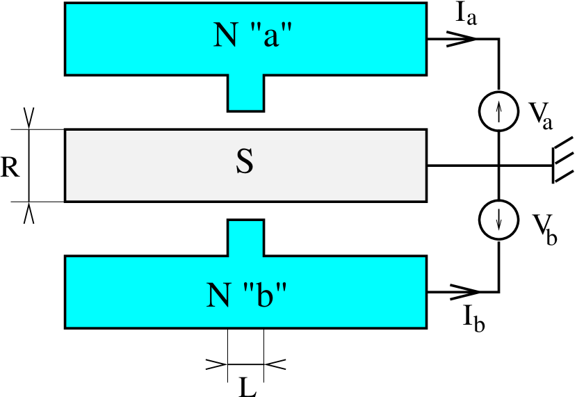
Figure 1: (Color online.) Schematic representation of the electrical circuit corresponding to the NISIN double interface interpolating between a localized contact for $L\sim\lambda_{F}$ (with $\lambda_{F}$ the Fermi wave-length) and and extended interface for $L\gg L_{\rm th}(\omega)$, where $L_{\rm th}$ is the Thouless length corresponding to the energy $eV_{b}$. The current $I_{a}$ through electrode “a” is determined in response to a voltage $V_{b}$ on electrode “b”, with $V_{a}=0$. The dimensions $R$ (superconductor thickness) and $L$ (dimension of the junction) are shown on the figure. The available experiment by Russo et al. Russo corresponds to extended interface with $L$ of the order of $0.5\mu$m and $R\simeq 15\div 200$nm.

The article is organized as follows. The factorization of non local processes as two local Andreev reflections and a non local propagation is discussed in Sec. II. The factorization of the non local conductance is illustrated in Sec. III in the case of one dimensional models (the Blonder, Thinkham, Klapwijk (BTK) modelBTK and a Green’s function model). The Thouless energy of non local conductance fluctuations is examined in Sec. IV on the basis of the evaluation of the diffuson. Numerical simulations are presented in Sec. V. The role of weak localization is pointed out in Sec. VI. Concluding remarks are given in Sec. VII.

II Factorization of the non local resistance

II.1 Existing results for $eV_{b}\gg E_{\rm th}(L)$

The diagram corresponding to the non vanishing lowest order process of order $T^{4}$ (with $T$ the normal transparency) is shown on Fig. 2a. This diagram is local with respect to excursions parallel to the interfaces if the bias voltage energy $eV_{b}$ is much larger than the Thouless energy $E_{\rm th}(L)$ associated to the dimension $L$ of the junction parallel to the interface (see Fig. 1), as it is the case in the experiment by Russo et al. Russo . The corresponding non local conductance

$$\overline{\cal G}_{a,b}(V_{b})=\frac{\partial I_{a}}{\partial V_{b}}(V_{b}),$$ (1)

where $I_{a}$ and $V_{b}$ are defined on Fig. 1, is given by Melin-Feinberg-PRB ; Melin-cond-mat

$$\overline{\cal G}_{a,b}(V_{b})=-\frac{e^{2}}{h}N_{\rm ch}T^{4}\frac{\xi}{l_{e}^{(S)}}\frac{\Delta^{2}}{\Delta^{2}-(eV_{b})^{2}}\exp{\left[-\left(\frac{2R}{\xi}\right)\right]},$$ (2)

where $N_{\rm ch}$ is the number of conduction channels, $\Delta$ the superconducting gap, $\xi$ the superconducting coherence length, $l_{e}^{(S)}$ the superconductor elastic mean free path, $T$ the normal local transparency, and the overline is an average over disorder. The local Andreev conductance is given by

$${\cal G}_{\rm loc}(V_{b})=2\frac{e^{2}}{h}N_{\rm ch}T^{2}\frac{\Delta^{2}}{\Delta^{2}-(eV_{b})^{2}},$$ (3)

where we used the ballistic result without disorder because of the condition $eV_{b}\gg E_{\rm th}(L)$.

The resistance matrix probed in the experiment Russo is the inverse of the conductance matrix calculated theoretically:

$$\left[\begin{array}[]{cc}{\cal R}_{a,a}(V_{b})&{\cal R}_{a,b}(V_{b})\\ {\cal R}_{b,a}(V_{b})&{\cal R}_{b,b}(V_{b})\end{array}\right]=\left[\begin{array}[]{cc}\overline{\cal G}_{a,a}(V_{b})&\overline{\cal G}_{a,b}(V_{b})\\ \overline{\cal G}_{b,a}(V_{b})&\overline{\cal G}_{b,b}(V_{b})\end{array}\right]^{-1},$$ (4)

from what we deduce that the non local resistance ${\cal R}_{a,b}(V_{b})$ is given by

$${\cal R}_{a,b}(V_{b})=\frac{-\overline{\cal G}_{a,b}(V_{b})}{[{\cal G}_{\rm loc}(V_{b})]^{2}-\overline{\cal G}_{a,b}(V_{b})\overline{\cal G}_{b,a}(V_{b})},$$ (5)

that simplifies into

$${\cal R}_{a,b}(V_{b})\simeq-\frac{\overline{\cal G}_{a,b}(V_{b})}{\left[{\cal G}_{\rm loc}(V_{b})\right]^{2}}$$ (6)

if the thickness of the superconductor is larger than the superconducting coherence length $\xi$, and leads to

$${\cal R}_{a,b}(V_{b}) = \frac{1}{4N_{\rm ch}}\frac{h}{e^{2}}\left(\frac{\xi}{l_{e}^{(S)}}\right)$$ (7)

$$\times \left(\frac{\Delta^{2}-(eV_{b})^{2}}{\Delta^{2}}\right)\exp{(-2R/\xi)}.$$

The non local resistance at low bias is positive (dominated by elastic cotunneling), as found in Ref. Melin-Feinberg-PRB, . The case of extended interfaces is addressed in Ref. Melin-cond-mat, .

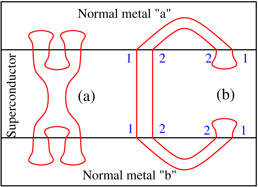
Figure 2: (Color online.) The diagrams representing the lowest order processes of order $T^{4}$. The diagram (a), local with respect to a propagation in the normal electrodes, was introduced in Ref. Melin-Feinberg-PRB, . The diagram (b) is its non local counterpart. “1” and “2” correspond to the electron and hole Nambu labels. The diagram on (b) factorizes in two Andreev reflections at both interfaces, and a non local propagation in the superconductor. The electron line crosses $8$ times the interfaces, so that the diagrams are of order $T^{4}$, where $T\propto(t/\epsilon_{F})^{2}$ is the normal transparency, with $t$ the tunnel amplitude and $\epsilon_{F}$ the Fermi energy.

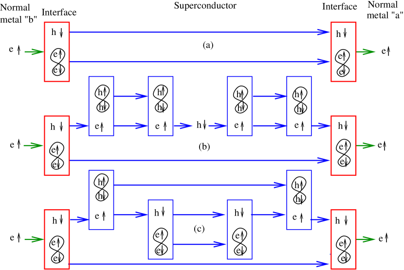
Figure 3: (Color online.) Schematic representation of (a): the formation of composite objects at the interfaces with a ballistic superconductor; (b): the sequential conversion of the composite objects in the bulk of the superconductor in the absence of weak localization; (c): the scattering induced by weak localization.

II.2 Case $eV_{b}\lesssim E_{\rm th}(L)$

Now, if the bias voltage energy $eV_{b}$ is smaller than the Thouless energy $E_{\rm th}(L)$, the lowest order diagram of order $T^{4}$ becomes non local in the normal electrodes (see Fig. 2b). The diagram on Fig. 2b corresponds to two Andreev reflections in the normal electrodes, connected by a propagation in the superconductor, so that the non local conductance factorizes into

$$\overline{\cal G}_{a,b}(V_{b})=\frac{{\cal S}(V_{b})\left[{\cal G}_{\rm loc}(V_{b})\right]^{2}}{N_{\rm ch}},$$ (8)

where ${\cal S}(V_{b})$ is a transmission coefficient of the superconductor. Using Eq. (6), we find that the crossed resistance

$${\cal R}_{a,b}(V_{b})=-\frac{{\cal S}(V_{b})}{N_{\rm ch}}$$ (9)

does not depend on the local conductances. The scaling between the local and non local conductances is tested in Sec. III for the generalization of the model of reflectionless tunneling at a single interface introduced by Melsen and Beenakker Melsen .

The factorization of the Andreev reflections at both interfaces suggests that part of the current is carried by pairs in the condensate. We thus arrive at the notion of the transport of a composite object made of an evanescent quasiparticle and a pair in the condensate: an electron from a normal electrode is transmitted in the superconductor as a quasi-hole and a pair in the condensate (see Fig. 3a). The consequences of this qualitative picture are considered below.

Finally, we note that the factorization of two Andreev reflections at the interfaces is also valid if $eV_{b}\gg E_{\rm th}(L)$ (see Sec. II.1), as in the experiment by Russo et al. Russo . This is because the normal Green’s functions are vanishingly small at zero energy in a superconductor.

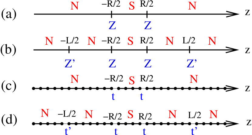
Figure 4: (Color online.) Schematic representations of the one dimensional models: (a) the BTK model for NISIN and (b) NINISININ junctions, and (c) the tight-binding model for NISIN and (d) NINISININ junctions.

III One dimensional models

III.1 Blonder, Tinkham, Klapwijk (BTK) approach

III.1.1 Non local conductance

Let us consider now a one dimensional model of NISIN double interface within the BTK approach japs (see Fig. 4a). The goal is two-fold: i) obtain the expression of the pair current in the superconductor, and ii) test the factorization of the non local conductance in the case of the model of reflectionless tunneling introduced by Melsen and Beenakker Melsen .

The gap of the superconductor is supposed to have a step-function variation as a function of the coordinate $z$ along the chain: $\Delta(z)=\Delta\theta(z+R/2)\theta(R/2-z)$, and we suppose $\delta$-function scattering potentials at the interfaces: $V(z)=H\delta(z+R/2)+H\delta(z-R/2)$ BTK . The interface transparencies are characterized by the parameter $Z=2mH/\hbar^{2}k_{F}$, where $v_{F}=\hbar k_{F}/m$ is the Fermi velocity, with $m$ the electron mass and $k_{F}$ the Fermi wave-vector. The one dimensional model is a simplified version of the genuine three terminal geometry with a supercurrent flow. The current in the normal electrode “a” is not equal to the injected current in electrode “b” because part of the injected current has been converted in a supercurrent.

The unknown coefficients in the expression of the wave-function are determined from the matching conditions at the interfaces BTK . Of particular interest are the amplitudes $a^{\prime}(k_{F}R)$ and $b^{\prime}(k_{F}R)$ of transmission in the electron-hole and electron-electron channels from one normal metal to the other, corresponding respectively to elastic cotunneling and non local Andreev reflection. Assuming $R\gg\xi$, we expand $a^{\prime}$ and $b^{\prime}$ to lowest order in $\exp{(-R/\xi)}$, to find the transmission coefficients

$$\int_{0}^{2\pi}\frac{d(k_{F}R)}{2\pi}|a^{\prime}(k_{F}R)|^{2}=$$ (10)

$$\left(\frac{1}{2Z^{4}}-\frac{1}{2Z^{6}}+\frac{1}{2Z^{8}}+...\right)e^{-2R/\xi}+{\cal O}\left(e^{-4R/\xi}\right)$$

$$\int_{0}^{2\pi}\frac{d(k_{F}R)}{2\pi}|b^{\prime}(k_{F}R)|^{2}=$$ (11)

$$\left(\frac{1}{2Z^{4}}-\frac{1}{2Z^{6}}+\frac{5}{4Z^{8}}+...\right)e^{-2R/\xi}+{\cal O}\left(e^{-4R/\xi}\right)$$

at $\omega=0$. We deduce the first non vanishing term in the large-$R$, large-$Z$ expansion of the non local transmission:

$$T^{\prime} = \int_{0}^{2\pi}\frac{d(k_{F}R)}{2\pi}\left(|a^{\prime}(k_{F}R)|^{2}-|b^{\prime}(k_{F}R)|^{2}\right)$$

$$= -\frac{3}{4Z^{8}}e^{-2R/\xi}+{\cal O}\left(e^{-4R/\xi}\right).$$

In agreement with the Green’s function approach Melin-Feinberg-PRB ; Melin-cond-mat corresponding to the diagrams on Fig. 2, the non local conductance is dominated by elastic cotunneling and appears at order $Z^{-8}\sim T^{4}$. In agreement with Ref. Melin-Feinberg-PRB, , we find no non local Andreev reflection for highly transparent interfaces corresponding to $Z=0$.

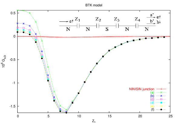
Figure 5: (Color online.) Variation of the non local conductance $G_{a,b}$ (in units of $e^{2}/h$) for the junction on Fig. 4c, with $Z^{\prime}=Z_{1}=Z_{4}$ and $Z=Z_{2}=Z_{3}=10$. (a) … (f) correspond to an increasing values of the precision in the evaluation of the Fermi phase factors related to the superconductor. We have also shown the much smaller non local conductance of the NINISIN junction, as a function of $Z_{1}$ for the NIN contact, with the same value of $Z$ for the NIS contacts.

III.2 Reflectionless tunneling

III.2.1 BTK approach

To discuss the form (9) of the crossed resistance, we include now multiple scattering in the normal electrodes and consider two additional scatterers at positions $z_{1}=-L_{1}/2$ in the left electrode and $z_{2}=L_{2}/2$ in the right electrode, described by the potentials $V^{\prime}(z)=H^{\prime}\delta(z-z_{1})+H^{\prime}\delta(z-z_{2})$, and leading to the barrier parameter $Z^{\prime}=2mH^{\prime}/\hbar^{2}k_{F}$ (see Fig. 4b for the definitions of $Z$ and $Z^{\prime}$). This constitutes, for a double interface, the analog of the model introduced by Melsen and Beenakker Melsen for a single interface. We average numerically the non local transmission coefficient over the Fermi oscillation phases $\varphi_{1}=k_{F}(R-L_{1})/2$, $\varphi=k_{F}R$ and $\varphi_{2}=k_{F}(L_{2}-R)$.

The variations of the non local conductance at zero bias as a function of $Z^{\prime}$ for a fixed $Z$ are shown on Fig. 5, as well as the corresponding non local conductance for the NINISIN junction. The negative non local conductance at small $Z_{1}$ for the NINISININ junction disappears when increasing the precision of the integrals. The variation of the non local conductance on Fig. 5 shows a strong enhancement by the additional scatterers, like reflectionless tunneling at a single NIS interface Melsen .

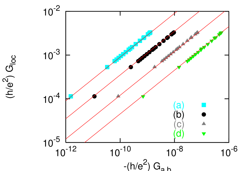
Figure 6: (Color online.) Correlation between the nonlocal conductance ($x$-axis) and the local conductance ($y$-axis) for the peaks similar to Fig. 5 as a function of $t^{\prime}/T$ for a fixed $t/T=0.05$ and (a) $R/\xi=5$, (b) $R/\xi=4$, (c) $R/\xi=3$, and (d) $R/\xi=2$. The solid line is a fit to ${\cal G}_{a,b}(t^{\prime}/T)\propto\left[G_{\rm loc}(t^{\prime}/T)\right]^{2}$.

III.2.2 Green’s functions: scaling between the local and non local conductances

Considering the tight-binding model within Green’s functions, the variation of the non local conductance of the NINISININ junction as a function of $t^{\prime}$ for a fixed $t$ (see Fig. 4d) is similar to the BTK model. Imposing the same normal conductance in the BTK and in the tight-binding models leads to $Z=(1-(t/T)^{2})/(2t/T)$, where $T$ is the bulk hopping amplitude. The identification of $Z$ to $t/T$ results in a good (but not perfect) agreement for the non local conductance when the tight-binding and BTK results are rescaled on each other. The non local conductance ${\cal G}_{a,b}(V_{b}=0,t/T,t^{\prime}/T)$ is shown on Fig. 6 as a function of the local conductance ${\cal G}_{\rm loc}(V_{b}=0,t/T,t^{\prime}/T)$, fitted by ${\cal G}_{a,b}(V_{b}=0,t/T,t^{\prime}/T)={\cal S}(V_{b}=0)\left[{\cal G}_{\rm loc}(V_{b}=0,t/T,t^{\prime}/T)\right]^{2}$, corresponding to Eq. (9) for $N_{\rm ch}=1$. The scaling is very well obeyed, showing the validity of form (9) of the crossed resistance involving the destruction of a pair in the condensate at one interface, its propagation in the superconductor and its creation at the other interface.

IV Thouless energy of a disordered superconductor

IV.1 Relevance to experiments

We consider now non local conductance fluctuations. The total non local transmission coefficient is given by $T_{tot}=T_{e-e}-T_{e-h}$, where $T_{e-e}$ and $T_{e-h}$ are the transmission coefficients in the electron-electron and electron-hole channels respectively. As discussed in Sec. II, one has $\overline{T_{tot}}=0$ but

$$\overline{\left(T_{tot}\right)^{2}}=\overline{\left(T_{e-e}\right)^{2}}+\overline{\left(T_{e-h}\right)^{2}}-2\overline{\left(T_{e-e}T_{e-h}\right)^{2}}.$$ (13)

Inspecting the corresponding lowest order diagrams shows that $\overline{T_{e-e}T_{e-h}}=-\overline{\left(T_{e-e}\right)^{2}}$, where we suppose that the normal metal phase coherence length is vanishingly small, therefore avoiding the specific effects of extended interfaces Melin-cond-mat . The root mean square of the non local conductance fluctuations is thus proportional to $(e^{2}/h)T^{2}$ while the average non local conductance is proportional to $(e^{2}/h)T^{4}N_{\rm ch}$ (see Eq. 2). The fluctuations are important for small junctions such that $T^{2}N_{\rm ch}\lesssim 1$.

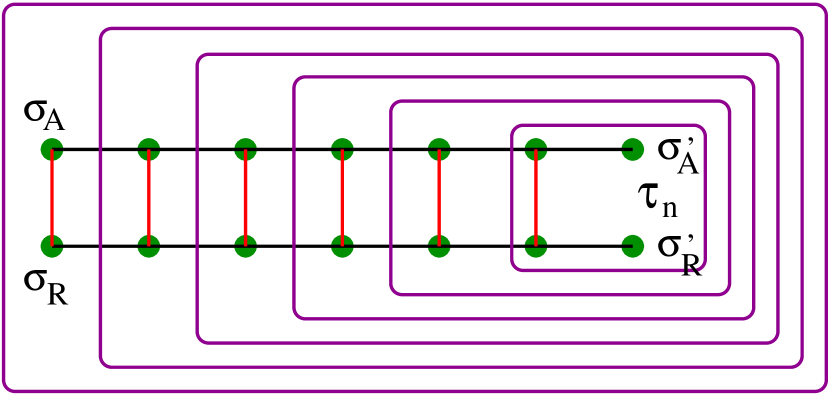
Figure 7: (Color online.) Schematic representation of the recursive calculation of the matrix diffuson in the ladder approximation used by Smith and Ambegaokar Smith . The integrals over the wave-vectors are carried out recursively, starting from the right of the diagram. The two horizontal black lines correspond to the advanced and retarded Green’s functions. The green dots correspond to the disorder vertices, and the vertical red lines correspond to the impurity lines. We have shown the Nambu labels $(\sigma_{A},\sigma_{R})$ and $(\sigma^{\prime}_{A},\sigma^{\prime}_{R})$ at the extremities of the diffuson.

IV.2 Diffusons in a superconductor

IV.2.1 Evaluation of the diffusons

Let us first evaluate the Thouless energy of a superconductor in the absence of crossings between diffusons. Smith and Ambegaokar Smith start from one extremity of the ladder diagram and calculate recursively the integrals over the wave-vectors. Once the right-most integral on Fig. 7 has been evaluated, one is left with a “ladder” with one less rung, but with a different $2\times 2$ matrix at the extremity. The four parameter recursion relations reduce to a matrix geometric series in the sector $(\hat{\tau}_{0},\hat{\tau}_{1})$, and to another matrix geometric series in the sector ($\hat{\tau}_{2}$,$\hat{\tau}_{3}$), where $\hat{\tau}_{n}$ are the four Pauli matrices, with $\hat{\tau}_{0}$ the identity.

More precisely, we define the four matrix diffusons

$$\overline{\hat{\cal D}}_{q,\delta\omega}(\hat{\tau}_{n})=v^{2}\int\frac{d^{3}{\bf k}}{(2\pi)^{3}}\overline{\hat{\tau}_{3}\hat{G}({\bf k},\omega)\hat{\tau}_{n}\hat{G}({\bf k}+{\bf q},\omega+\delta\omega)\hat{\tau}_{3}},$$ (14)

where $n=0,...,3$, $q=|{\bf q}|$ is the modulus of the wave-vector, and $\delta\omega$ is small compared to the energy $\omega$. The microscopic disorder scattering potential is given by $v^{2}=4\pi\epsilon_{F}/\tau_{e}$, with $\epsilon_{F}$ the Fermi energy and $\tau_{e}$ the elastic scattering time, related to the elastic scattering length $l_{e}$ by the relation $l_{e}=v_{F}\tau_{e}$. We find

$$\overline{\hat{\cal D}}_{q,\delta\omega}(\hat{\tau}_{0}) = X\left(\Delta^{2}\hat{\tau}_{0}-\omega\Delta\hat{\tau}_{1}\right)$$ (15)

$$\overline{\hat{\cal D}}_{q,\delta\omega}(\hat{\tau}_{1}) = X\left(\omega\Delta\hat{\tau}_{0}-\omega^{2}\hat{\tau}_{1}\right),$$ (16)

in the sector $(\hat{\tau}_{0},\hat{\tau}_{1})$, and

$$\overline{\hat{\cal D}}_{q,\delta\omega}(-i\hat{\tau}_{2})=X\left(-\frac{3{\cal D}_{0}\Delta\delta\omega\sqrt{\Delta^{2}-\omega^{2}}}{2v_{F}^{2}}\hat{\tau}_{3}-\right.$$ (17)

$$\left.i(\Delta^{2}-\omega^{2})\hat{\tau}_{2}\right)$$

$$\overline{\hat{\cal D}}_{q,\delta\omega}(\hat{\tau}_{3})=X{\cal D}_{0}\delta\omega\left(-\frac{{\cal D}_{0}^{2}\Delta\delta\omega}{4v_{F}^{4}}\hat{\tau}_{3}-\frac{3i\Delta}{2v_{F}^{2}}\sqrt{\Delta^{2}-\omega^{2}}\hat{\tau}_{2}\right),$$

in the sector $(\hat{\tau}_{2},\hat{\tau}_{3})$. We used the notation

$$\frac{1}{X}=\frac{3{\cal D}_{0}(\Delta^{2}-\omega^{2})}{v_{F}^{2}}\left[\sqrt{\Delta^{2}-\omega^{2}}+\frac{{\cal D}_{0}q^{2}}{4}-\frac{\omega\delta\omega}{2\sqrt{\Delta^{2}-\omega^{2}}}\right],$$ (18)

where ${\cal D}_{0}$ is the diffusion constant.

IV.2.2 Non local transmission coefficient

The relation between the diffusons in the superconductor and non local transport is provided by the non local conductance (1). The non local conductance ${\cal G}_{a,b}^{(2)}(\omega)$ of order $T^{2}$ is related to the transmission coefficients according to

$${\cal G}_{a,b}^{(2)}(\omega)=\frac{e^{2}}{h}\left[T_{(1,1)}^{(1,1)}(\omega)-T_{(1,1)}^{(2,2)}(\omega)\right],$$ (19)

with

$$T_{(\sigma_{A},\sigma_{R})}^{(\sigma^{\prime}_{A},\sigma^{\prime}_{R})}(\omega)=T^{2}\epsilon_{F}^{2}\int\frac{d^{3}{\bf q}}{(2\pi)^{3}}e^{i{\bf q}.{\bf R}}$$ (20)

$$\times\int\frac{d^{3}{\bf k}}{(2\pi)^{3}}\overline{\hat{G}^{\sigma_{A},\sigma^{\prime}_{A}}({\bf k},\omega)\hat{G}^{\sigma^{\prime}_{R},\sigma_{R}}({\bf k}+{\bf q},\omega)}.$$

The notation $T_{(\sigma_{A},\sigma_{R})}^{(\sigma^{\prime}_{A},\sigma^{\prime}_{R})}(\omega)$ corresponds to the transmission coefficient related to a diffuson with the Nambu labels $(\sigma_{A},\sigma_{R})$ for the advanced and retarded propagators at one extremity, and the Nambu labels $(\sigma^{\prime}_{A},\sigma^{\prime}_{R})$ at the other extremity (see Fig. 7). The transmission coefficients $\overline{T}_{(1,1)}^{(1,1)}(\omega)$ and $\overline{T}_{(1,1)}^{(2,2)}(\omega)$ encode elastic cotunneling and non local Andreev reflection respectively. With the notations in Sec. IV.1, we have $\overline{T}_{(1,1)}^{(1,1)}(\omega)=T_{e-e}(\omega)$ for transmission in the electron-electron channel, and $\overline{T}_{(1,1)}^{(2,2)}(\omega)=T_{e-h}(\omega)$ for transmission in the electron-hole channel. We deduce from Eq. (IV.2.1) that $\overline{\cal G}^{(2)}_{a,b}(\omega)=0$: the average non local conductance vanishes to order $T^{2}$, in agreement both with Sec. II and with an early work Feinberg-des in the disordered case. The transmission coefficients $\overline{T}_{(1,2)}^{(1,2)}(\omega)$ and $\overline{T}_{(2,1)}^{(2,1)}(\omega)$ involve the propagation of a pair in the condensate in parallel to the quasiparticle channels, as in the diagram on Fig. 2b.

IV.3 Thouless energy

The Thouless energy is defined from the non local conductance fluctuations by the decay of the autocorrelation of the non local conductance

$$\langle\left[\overline{{\cal G}_{a,b}(\omega){\cal G}_{a,b}(\omega+\delta\omega)}-\overline{\cal G}_{a,b}(\omega)\overline{\cal G}_{a,b}(\omega+\delta\omega)\right]\rangle_{\omega}$$ (21)

as $\delta\omega$ increases, where $\langle...\rangle_{\omega}$ denotes an average over the energy $\omega$ in a given window.

The autocorrelation of the non local conductance defined by Eq. (21) is related to the autocorrelation of the transmission coefficients

$$\langle\overline{T_{(\sigma_{1},\sigma_{2})}^{(\sigma^{\prime}_{1},\sigma^{\prime}_{2})}(\omega)T_{(\sigma_{3},\sigma_{4})}^{(\sigma^{\prime}_{3},\sigma^{\prime}_{4})}(\omega+\delta\omega)}$$ (22)

$$-\overline{T}_{(\sigma_{1},\sigma_{2})}^{(\sigma^{\prime}_{1},\sigma^{\prime}_{2})}(\omega)\overline{T}_{(\sigma_{3},\sigma_{4})}^{(\sigma^{\prime}_{3},\sigma^{\prime}_{4})}(\omega+\delta\omega)\rangle_{\omega}.$$

More precisely, the non local conductance to lowest order in the tunnel amplitudes is given by

$${\cal G}_{a,b}(\omega)={\cal A}\left[g_{a,b}^{1,1,A}g_{b,a}^{1,1,R}-g_{a,b}^{1,2,A}g_{b,a}^{2,1,R}\right],$$ (23)

where “1” and “2” refer to the electron and hole Nambu components, “A” and “R” stand for advanced and retarded, $g_{a,b}^{1,1}$ is a propagation from “a” to “b” in the electron-electron channel, and $g_{a,b}^{1,2}$ in the electron-hole channel. The prefactor ${\cal A}$, not directly relevant to our discussion, can be found in Ref. Melin-Feinberg-PRB, . We find easily

$$\overline{{\cal G}_{a,b}(\omega){\cal G}_{a,b}(\omega+\delta\omega)}={\cal A}^{2}\sum_{k_{1},...,k_{4}}e^{i(k_{1}-k_{2}+k_{3}-k_{4})R}$$

$$\left[\overline{g^{A}_{1,1}(k_{1},\omega)g^{R}_{1,1}(k_{2},\omega)g^{A}_{1,1}(k_{3},\omega+\delta\omega)g^{R}_{1,1}(k_{4},\omega+\delta\omega)}\right.$$

$$- \overline{g^{A}_{1,1}(k_{1},\omega)g^{R}_{1,1}(k_{2},\omega)g^{A}_{1,2}(k_{3},\omega+\delta\omega)g^{R}_{2,1}(k_{4},\omega+\delta\omega)}$$

$$- \overline{g^{A}_{1,2}(k_{1},\omega)g^{R}_{2,1}(k_{2},\omega)g^{A}_{1,1}(k_{3},\omega+\delta\omega)g^{R}_{1,1}(k_{4},\omega+\delta\omega)}$$

$$+ \left.\overline{g^{A}_{1,2}(k_{1},\omega)g^{R}_{2,1}(k_{2},\omega)g^{A}_{1,2}(k_{3},\omega+\delta\omega)g^{R}_{2,1}(k_{4},\omega+\delta\omega)}\right].$$

The quantity

$${\cal S}_{a,b}(\omega,\omega+\delta\omega)=\overline{{\cal G}_{a,b}(\omega){\cal G}_{a,b}(\omega+\delta\omega)}-\overline{{\cal G}_{a,b}(\omega){\cal G}_{a,b}(\omega)}$$ (25)

is evaluated by discarding the Nambu components of the type $\overline{g^{A}_{1,1}(k_{1},\omega)g^{A}_{1,2}(k_{2},\omega+\delta\omega)}$, much smaller than $\overline{g^{A}_{1,1}(k_{1},\omega)g^{A}_{1,1}(k_{2},\omega+\delta\omega)}$ and $\overline{g^{A}_{1,2}(k_{1},\omega)g^{A}_{2,1}(k_{2},\omega+\delta\omega)}$ if $\omega$ is small compared to $\Delta$. In addition, we use

$$\overline{{\cal G}_{a,b}(\omega){\cal G}_{a,b}(\omega)}\simeq\overline{{\cal G}_{a,b}(\omega+\delta\omega){\cal G}_{a,b}(\omega+\delta\omega)}$$ (26)

within the small energy window that we consider. We obtain

$${\cal S}_{a,b}(\omega,\omega+\delta\omega)=$$

$$2\left(T_{(1,1)}^{(1,1)}(R,\omega,\delta\omega)\right)^{2}+2\left(T_{(1,1)}^{(2,2)}(R,\omega,\delta\omega)\right)^{2}$$

$$- 2\left(T_{(1,1)}^{(1,1)}(R,\omega,0)\right)^{2}-2\left(T_{(1,1)}^{(2,2)}(R,\omega,0)\right)^{2},$$

where the Fourier transforms with respect to the spatial variable of $T_{(1,1)}^{(1,1)}(R,\omega,\delta\omega)$ and $T_{(1,1)}^{(2,2)}(R,\omega,\delta\omega)$ are given by

$$T_{(1,1)}^{(1,1)}(q,\omega,\delta\omega)=T_{(1,1)}^{(2,2)}(q,\omega,\delta\omega)=$$ (28)

$$\frac{v_{F}^{2}\Delta^{2}}{3{\cal D}_{0}^{2}(\Delta^{2}-\omega^{2})\left[\sqrt{\Delta^{2}-\omega^{2}}+{\cal D}_{0}q^{2}/4-\omega\delta\omega/2\sqrt{\Delta^{2}-\omega^{2}}\right]},$$

deduced from Sec. IV.2.1. The notation $R$ stands for the distance between the contacts “a” and “b”. Taking the Fourier transform of Eq. (28), we obtain

$${\cal S}_{a,b}(\omega,\delta\omega)\left[\overline{{\cal G}_{a,b}(\omega){\cal G}_{a,b}(\omega)}\right]^{-1}$$

$$= \exp{\left(i\sqrt{3}\frac{R}{\xi}\frac{\omega\delta\omega}{4(\Delta^{2}-\omega^{2})}\right)}-1,$$

that dephases above the Thouless energy

$$E_{c}=\delta\omega_{c}=\frac{8\pi}{\sqrt{3}}\frac{\Delta^{2}-\omega^{2}}{\omega}\frac{\xi}{R},$$ (30)

for energies $\omega$ large compared to $\Delta\sqrt{\xi/R}$, so that $E_{c}$ is much smaller than $\omega$.

V Numerical results

V.1 The different length scales in the simulations

The non local transport simulations are carried out in a quasi-1D geometry, on a strip of longitudinal dimension $L$ and of transverse dimension $L_{y}$, corresponding to $M$ transverse modes. We calculate non local transport along the $z$ direction. The trilayer geometry with an aspect ratio similar to the experiment by Russo et al. Russo , would require much larger system sizes to have a reasonable separation between the different length scales in the $y$ direction while $L$ is much larger than $L_{y}$. The relevant length scales in the diffusive regime are given by increasing order by the Fermi wave-length $\lambda_{F}$, the elastic mean free path $l_{e}$, the superconducting coherence length $\xi$ and the sample size.

V.2 Ballistic system and small disorder

We use typically $M=10$, $L/a_{0}$ ranging from $80$ to $100$ for a method Levy-Yeyati based on the inversion of the Dyson matrix, and much higher values of $L/a_{0}$ (in units of the tight binding model lattice spacing $a_{0}$), for a complementary method consisting in connecting together several conductors by a hopping self-energy, given the Green’s functions of each conductor evaluated by the inversion of the Dyson matrix. Disorder is introduced as in the Anderson model by a random potential between $-W$ and $W$.

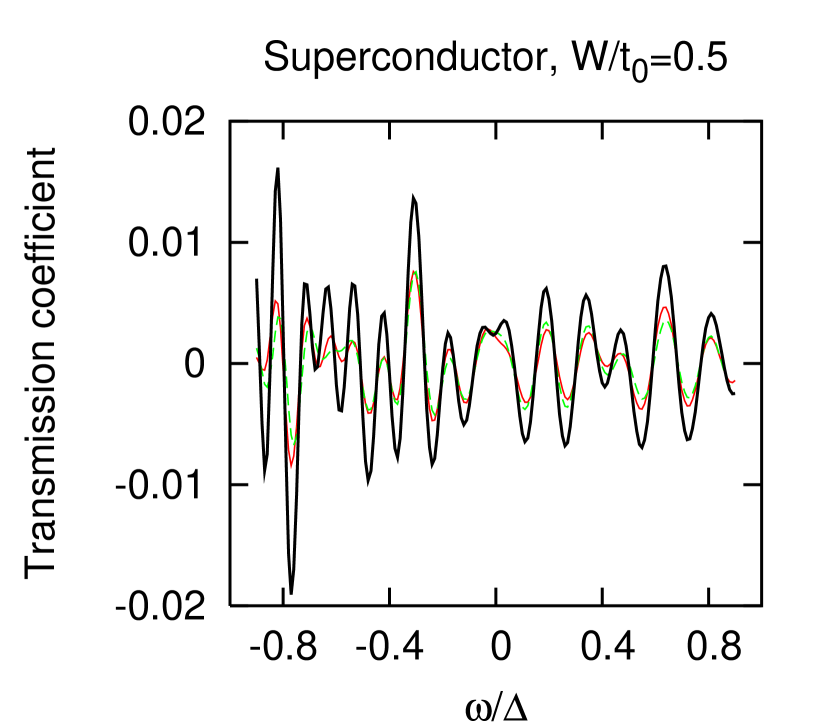
Figure 8: (Color online.) Energy dependence of the superconducting transmission coefficient $T^{\prime}(\omega/\Delta)$ [defined by Eq. (31)] through a diffusive superconductor on a strip with $L_{y}/a_{0}=10$ and $L/a_{0}=100$, in the limit of small disorder. The bold line corresponds to the ballistic result, and the two other traces correspond to two realizations of disorder with $W/t_{0}=0.5$ and $l_{e}/a_{0}\simeq 500$. The ballistic coherence length is $\xi/a_{0}\simeq 33$. This figure has been obtained with a method based on the inversion of the Dyson matrix.

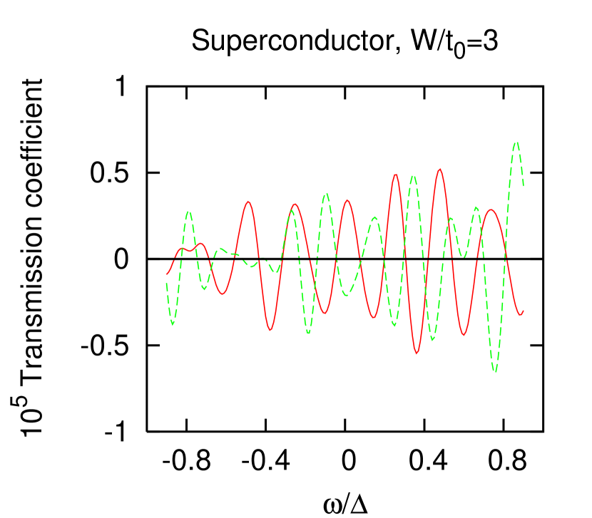
Figure 9: (Color online.) Energy dependence of the superconducting transmission coefficient $T^{\prime}(\omega/\Delta)$ [defined by Eq. (31)] through a diffusive superconductor on a strip with $L_{y}/a_{0}=10$ and $L/a_{0}=100$, in the diffusive limit. The two traces correspond to different realizations of disorder corresponding to $W/t_{0}=3$ and $l_{e}/a_{0}\simeq 16$. This figure has been obtained with a method based on the inversion of the Dyson matrix.

The normalized transmission coefficient $T^{\prime}(\omega)$ that we calculate numerically is related to the non local conductance by the relation

$$T^{\prime}(\omega)=\frac{h}{e^{2}}T^{-2}{\cal G}_{a,b}^{(2)}(\omega),$$ (31)

where ${\cal G}_{a,b}^{(2)}(\omega)$ is the contribution of order $T^{2}$ to the non local conductance, with $T$ the normal transparency. The transmission coefficient $T^{\prime}(\omega)$ defined by Eq. (31) fluctuates around zero as a function of energy because the wave-vectors of the different channels vary with energy. The characteristic energy scale in the oscillations of the transmission coefficient is the ballistic normal state Thouless energy associated to the dimension $L$ (see Fig. 8 in the forthcoming section V.3).

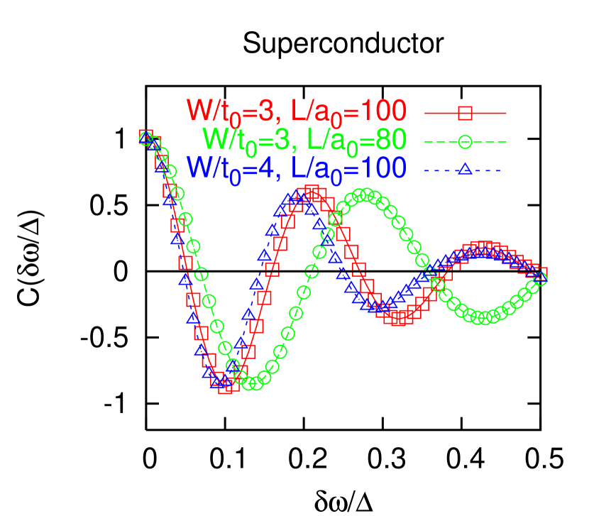
Figure 10: (Color online.) Autocorrelation function of the transmission coefficient [see Eqs. (32)-(33)], for ($W/t_{0}=3$, $L/a_{0}=80$), ($W/t_{0}=3$, $L/a_{0}=100$), and ($W/t_{0}=4$,$L/a_{0}=100$). $W/t_{0}=3$ corresponds to $l_{e}/a_{0}\simeq 16$, and $W/t_{0}=4$ corresponds to $l_{e}/a_{0}\simeq 10$. The errorbars are smaller than the size of the symbols.

V.3 Thouless energy of a disordered superconductor

Figs. 8 and 9 show the energy dependence of the superconducting transmission coefficient $T^{\prime}(\omega/\Delta)$ defined by Eq. (31). The fluctuations of the transmission coefficient are close to the ballistic limit result in the limit of small disorder (see Fig. 8). We obtain regular fluctuations of the transmission coefficient of a superconductor in the diffusive limit where the normal transmission coefficient is characterized by fluctuations (see Fig. 9). We used a large number of realizations of disorder at a single energy to show that the transmission coefficient averages to zero because of disorder. This shows that the regular fluctuations in the disordered system are genuinely related to disorder, and do not have the same origin as in the ballistic system.

To characterize the regular fluctuations, we calculate the normalized autocorrelation of the transmission coefficient ${\cal C}(\delta\omega)=\langle A(\omega,\delta\omega)/B(\omega,\delta\omega)\rangle_{\omega}$, with

$$A(\omega,\delta\omega) = \overline{T^{\prime}(\omega+\delta\omega)T^{\prime}(\omega)}$$ (32)

$$B(\omega,\delta\omega) = \sqrt{\overline{T^{\prime}}(\omega+\delta\omega)\overline{T^{\prime}}(\omega)},$$ (33)

where $\langle...\rangle_{\omega}$ is an average over the energy $\omega$, as in Eq. (21). The autocorrelation ${\cal C}(\delta\omega)$ is characterized by oscillatory damped oscillations (see Fig. 10), in contrast to the autocorrelation of conductance fluctuations in the normal case that is damped without oscillations. The energy scales $E_{c,1}$ and $E_{c,2}$ related to period of oscillations and to the damping increase as the system size decreases (see Fig. 10), in agreement with the expected behavior for Thouless-like energies. Going to larger system sizes, we find that $E_{c,1}$ scales like the inverse of the sample size (see Fig. 11).

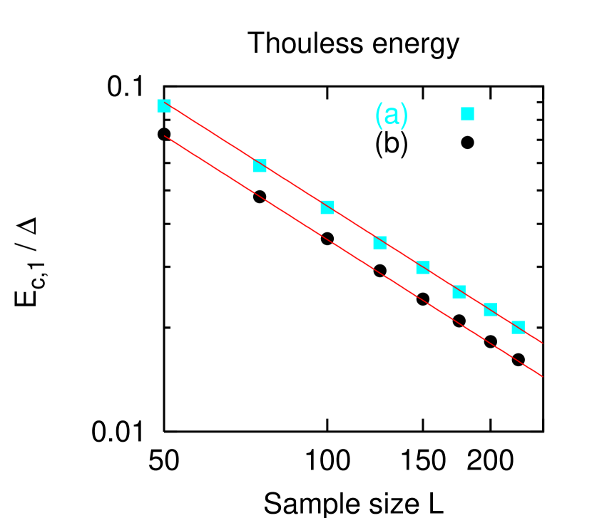
Figure 11: (Color online.) Variation of the Thouless energy $E_{c,1}/\Delta$ as a function of the system size $L/a_{0}$ in a log-log plot, for (a): $W/t=1$ and $l_{e}/a_{0}\simeq 127$ (b): $W/t=2$ and $l_{e}/a_{0}\simeq 34$. The solid lines are a fit to $E_{c,a}/\Delta\sim 1/L$.

The comparison between Fig. 9 for ($W/t_{0}=3$, $l_{e}/a_{0}\simeq 16$), and similar data for ($W/t_{0}=2$, $l_{e}/a_{0}\simeq 34$) and ($W/t_{0}=4$, $l_{e}/a_{0}\simeq 10$) show that $E_{c,1}$ and $E_{c,2}$ have a weaker dependence on the elastic mean free path than for a normal diffusive system.

VI Effective scattering induced by weak localization

We find a formal analogy between the calculation of the non local conductance fluctuations in the preceding section, and the linear response theory of collective modes Anderson ; Bogoliubov ; Kulik . Namely, the non local conductance fluctuations can be viewed as a generalized susceptibility in linear response, but otherwise the two models involve rather different physical quantities. We show now that weak localization can induce additional couplings to the condensate. Evaluating all the Nambu labels at the two three-diffuson vertices (see Fig. 12c) is possible in the limit $\omega\ll\Delta$ because of the constraint that the normal local Green’s functions can be discarded in this limit that corresponds “internal” Andreev reflection processes as on Fig. 3c. The diagrams on Fig. 12c then defines a set of transmission coefficients modified by weak localization. With the notations $A=T_{(1,2)}^{(1,2)}$, $B=T_{(1,2)}^{(2,1)}$, $C=T_{(1,1)}^{(2,2)}$, $D=T_{(1,1)}^{(1,1)}$, we find for the “renormalized” transmission coefficients

$$\tilde{A} = A+\lambda\left[AB(A+B)^{2}+D^{2}(A^{2}+B^{2})\right.$$

$$+ \left.2ABC^{2}\right]+{\cal O}(\lambda^{2})$$

$$\tilde{B} = B+\lambda\left[AB(A+B)^{2}+C^{2}(A^{2}+B^{2})\right.$$

$$+ \left.2ABD^{2}\right]+{\cal O}(\lambda^{2})$$

$$\tilde{C} = C+\lambda D(A+B)(D^{2}+3C^{2})+{\cal O}(\lambda^{2})$$ (36)

$$\tilde{D} = D+\lambda C(A+B)(C^{2}+3D^{2})+{\cal O}(\lambda^{2}),$$ (37)

with the perturbative parameter $\lambda\sim(\tau^{2}\epsilon_{F}\Delta)^{-4}$ that can turn out to be large. Weak localization can thus lead to a large effective scattering for the processes on Fig. 3c with multiple imbricate Andreev reflections providing a coupling between the condensate and the evanescent quasiparticle channels.

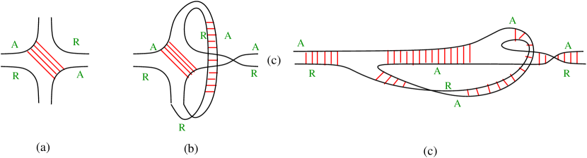
Figure 12: (Color online.) (a) One of the Gorkov-Larkin-Khmelnitskii-Hikami (GLKH) boxes Gorkov ; Hikami ; Montambaux in the superconducting case, dressed by a diffuson. (b) The self-crossing of a diffuson with the superconducting GLKH box. (c) Another representation of (b), with two additional diffusons at the entry and exit of the GLKH box. “A” and “R” stand for advanced and retarded.

VII Conclusions

To conclude, we have provided a theory of non local conductance fluctuations at normal metal / superconductor double interfaces. First, reconsidering the case of the average non local conductance, we confirm that the central role is played by higher order processes in the tunnel amplitude. We found that for these processes part of the non local current circulates as pairs in the condensate, not only as evanescent quasiparticles. The crossed conductance at zero bias factorizes in the Andreev conductances at the two interfaces, and a factor related to the propagation in the superconductor. This factorization was tested in the context of a model of reflectionless tunneling Melsen .

On the other hand we found numerically regular fluctuations of the non local conductance. The Thouless energy inverse proportional to the system size obtained in the simulations can be interpreted by a model ignoring weak localization. Alternatively, an energy scale inverse proportional to the system size could have received an interpretation in terms of the AndersonAnderson -BogoliubovBogoliubov collective mode, which is not in contradiction with the fact that weak localization can induce a strong coupling to the condensate if the superconductor elastic mean free path is sufficiently small. However, disorder in our simulations is most likely not strong enough to correspond to this possibility. Finally, the Thouless energy of a normal cavity appears also in circuit theoryMorten . Our model for the conductance fluctuations clarifies the concept of Thouless energy intrinsic to a superconductor.

References

- (1) U.P.R. 5001 du CNRS, Laboratoire conventionné avec l’Université Joseph Fourier
- (2) A.F. Andreev, Sov. Phys. JETP 19, 1228 (1964).
- (3) C.J. Lambert and R. Raimondi, J. Phys.: Condens. Matter 10, 901 (1998).
- (4) F.J. Jedema et al., Phys. Rev. B 60, 16549 (1999).
- (5) M.S. Choi, C. Bruder, and D. Loss, Phys. Rev. B 62, 13569 (2000); P. Recher, E. V. Sukhorukov, and D. Loss Phys. Rev. B 63, 165314 (2001)
- (6) G. B. Lesovik, T. Martin, and G. Blatter, Eur. Phys. J. B 24, 287 (2001); N. M. Chtchelkatchev, G. Blatter, G. B. Lesovik, and T. Martin, Phys. Rev. B 66, 161320(R) (2002).
- (7) J. M. Byers and M. E. Flatté, Phys. Rev. Lett. 74, 306 (1995).
- (8) G. Deutscher and D. Feinberg, App. Phys. Lett. 76, 487 (2000);
- (9) P. Samuelsson, E. V. Sukhorukov, and M. Büttiker, Phys. Rev. Lett. 91, 157002 (2003).
- (10) E. Prada and F. Sols, Eur. Phys. J. B 40, 379 (2004).
- (11) C. J. Lambert, J. Koltai, and J. Cserti, Towards the Controllable Quantum States (Mesoscopic Superconductivity and Spintronics, 119, Eds H. Takayanagi and J. Nitta, World Scientific (2003).
- (12) R. Mélin and S. Peysson, Phys. Rev. B 68, 174515 (2003); R. Mélin, Phys. Rev. B 72, 134508 (2005).
- (13) G. Falci, D. Feinberg, and F.W.J. Hekking, Europhysics Letters 54, 255 (2001).
- (14) D. Feinberg, Eur. Phys. J. B 36, 419 (2003).
- (15) N. M. Chtchelkatchev and I. S. Burmistrov, Phys. Rev. B 68, 140501 (2003).
- (16) R. Mélin and D. Feinberg, Eur. Phys. J. B 26, 101 (2002).
- (17) R. Mélin and D. Feinberg, Phys. Rev. B 70, 174509 (2004).
- (18) F. Taddei and R. Fazio, Phys. Rev. B 65, 134522 (2002).
- (19) G. Bignon, M. Houzet, F. Pistolesi, and F. W. J. Hekking, Europhys. Lett. 67, 110 (2004).
- (20) R. Mélin, Phys. Rev. B 73, 174512 (2006).
- (21) D. Beckmann, H.B. Weber, and H. v. Löhneysen, Phys. Rev. Lett. 93, 197003 (2004). D. Beckmann and H. v. Löhneysen, LT 24 conference proceedings, cond-mat/0512445 (2005).
- (22) S. Russo, M. Kroug, T.M. Klapwijk, and A.F. Morpugo, Phys. Rev. Lett. 95, 027002 (2005).
- (23) G.E. Blonder, M. Tinkham, and T.M. Klapwijk, Phys. Rev. B 25, 4515 (1982).
- (24) J.A. Melsen and C.W.J. Beenakker, Physica (Amsterdam) 203B, 219 (1994).
- (25) T. Yamashita, S. Takahashi and S. Maekawa, Phys. Rev. B 68, 174504 (2003); Phys. Rev. B 67, 094515 (2003).
- (26) R. A. Smith and V. Ambegaokar, Phys. Rev. B 45, 2463 (1992).
- (27) Normal state universal conductance fluctuations were obtained with the same parameters and with a recursive method [A. Levy Yeyati, Phys. Rev. B 45, 14189 (1992)].
- (28) P.W. Anderson, Phys. Rev. 110, 827 (1958); Phys. Rev. 112, 1900 (1958).
- (29) N. N. Bogoliubov, J. Exptl. Theoret. Phys. U.S.S.R. 34, 73 (1958); [Soviet Phys. JETP 34(7), 51 (1958)].
- (30) I.O. Kulik, O. Entin-Wohlman and R. Orbach, Jour. Low Temp. Phys. 43, 591 (1981).
- (31) L.P. Gorkov, A. Larkin, and D.E. Khmelnitskii, Pis’ma Zh. Eksp. Teor. Fiz 30, 248 (1979) [JETP Lett. 30, 228 (1979)].
- (32) S. Hikami, Phys. Rev. B 24, 2671 (1981).
- (33) E. Akkermans and G. Montambaux, Physique mésoscopique des électrons et des photons, CNRS Editions, EDP Sciences (2004).
- (34) J.P. Morten, A. Brataas, and W. Belzig, cond-mat/0606561.