Non–equilibrium Anisotropic Phases, Nucleation and Critical Behavior in a Driven Lennard–Jones Fluid

Abstract

We describe short–time kinetic and steady–state properties of the non–equilibrium phases, namely, solid, liquid and gas anisotropic phases in a driven Lennard–Jones fluid. This is a computationally–convenient two-dimensional model which exhibits a net current and striped structures at low temperature, thus resembling many situations in nature. We here focus on both critical behavior and details of the nucleation process. In spite of the anisotropy of the late–time “spinodal decomposition” process, earlier nucleation seems to proceed by Smoluchowski coagulation and Ostwald ripening, which are known to account for nucleation in equilibrium, isotropic lattice systems and actual fluids. On the other hand, a detailed analysis of the system critical behavior rises some intriguing questions on the role of symmetries; this concerns the computer and field–theoretical modeling of non-equilibrium fluids.

I Introduction

Steady states in non–equilibrium many–particle systems typically involve a constant flux of matter, charge, or some other quantity and, consequently, stripes or other spatial anisotropies show up at appropriate scales haken ; garr ; cross ; Marro . This occurs during segregation in driven sheared systems exp ; beysens2 ; follow , flowing fluids rheology2 , shaken granular matter reis ; sanchez , and non–equilibrium liquid–liquid binary mixtures liqliq , and it has been reproduced in computer simulations of driven colloidal loewen3 and fluid Marro ; hurtado systems, for instance. Further examples are the anisotropies observed in both high–temperature superconductors cuprates0 ; cuprates1 and electron gases 2deg1 ; mosfet . The ripples shaped by the wind in sand deserts dunes ; dunes2 and the lanes and trails formed by living organisms and vehicle traffic helbing ; lanes also share some of the essential physics.

Lacking theory for the “thermodynamic” instabilities causing the observed striped structures, one tries to link them to the microscopic dynamics of suitable model systems. For two decades, the driven lattice gas (DLG) KLS , namely, a computationally–convenient model system in which particles diffuse under an external driving “field”, has been a theoretical prototype of anisotropic behavior Marro ; Zia ; odor . This model was recently shown to be unrealistic in some essential sense, however manolo0 . Particle moves in the DLG are along the principal lattice directions, and any site can hold one particle at most, so that a particle impedes the one behind to jump freely along the direction which is favored to model the action of the field. Consequently, the lattice geometry acts more efficiently in the DLG as an ordering agent than the field itself, which occurs rarely —never so dramatically— in actual cooperative transport. In fact, actual situations may in principle be more closely modeled by means of continuum models, and this peculiarity of the DLG implies that it lacks a natural off-lattice extension manolo0 .

Here we present, and analyze numerically a novel non–equilibrium off-lattice, Lennard–Jones (LJ) system which is a candidate to portray some of the anisotropic behavior in nature. The model, which involves a driving field of intensity $E,$ reduces to the celebrated (equilibrium) LJ fluid smit ; Allen as $E\rightarrow 0.$ For any $E>0,$ however, it exhibits currents and anisotropic phases as in many observations out of equilibrium. In particular, as the DLG, our model in two dimensions shows striped steady states below a critical point. We also observe critical behavior consistent with the equilibrium universality class. This is rather unexpected in view of the criticality reported both for the DLG and in a related experiment exp . On the other hand, concerning the early–time relaxation before well–defined stripes form by spinodal decomposition, we first observe —as in previous studies of relaxation towards equilibrium— effective diffusion of small droplets, which is followed by monatomic diffusion probably competing with more complex processes. It is very likely that our observations here concerning nucleation, coexistence, criticality, and phases morphology hold also in a number of actual systems.

The paper is organized as follows. In section II we define the model, and section III is devoted to the main results as follows. § III.A describes the early–time segregation process as monitored by the excess energy, which measures the droplets surface. § III.B describes some structural properties of the steady state, namely, the radial and azimuthal distribution functions, and the degree of anisotropy. § III.C, which depicts some transport properties, is devoted to an accurate estimate of the liquid–vapor coexistence curve and the associated critical indexes. Section IV contains a brief conclusion.

II The model

Consider $N$ particles of equal mass (set henceforth to unity) in a $d-$dimensional box, $L^{d},$ with periodic boundary conditions. Interactions are via the truncated and shifted pair potential Allen :

$$\phi(r)=\left\{\begin{array}[]{cc}\phi_{LJ}(r)-\phi_{LJ}(r_{c})&\text{if }r<r_{c}\\ 0&\text{if }r\geqslant r_{c},\end{array}\right.$$ (1)

where

$$\phi_{LJ}(r)=4\epsilon\left[(\sigma/r)^{12}-(\sigma/r)^{6}\right]$$ (2)

is the LJ potential, $r$ stands for the interparticle distance, and $r_{c}$ is a cut-off that we set $r_{c}=2.5\sigma$. The parameters $\sigma$ and $\epsilon$ are, respectively, the characteristic length and energy —that we use in the following to reduce units as usual.

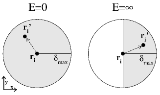
Figure 1: Schematic representation of the region (grey) which is accesible to a given particle as a consequence of a trial move for $E=0$ (left) and $E=\infty$ (right), assuming the “infinite” field points $\hat{x},$ horizontally.

Time evolution is by microscopic dynamics according to the transition probability per unit time (rate):

$$\omega^{\left(E\right)}\left(\mathbf{\eta}\rightarrow\mathbf{\eta}_{i}\right)=\chi^{(E)}\times\min\left\{1,e^{-\Delta\Phi_{i}/T}\right\}.$$ (3)

Here,

$$\chi^{(E)}=\frac{1}{2}\left[1+\tanh\left(E\hat{x}\cdot\vec{\delta}_{i}\right)\right],$$ (4)

$E$ is the intensity of a uniform external field along a principal lattice direction, say $\hat{x},$ $\mathbf{\eta}\equiv\left\{\vec{r}_{1},\ldots,\vec{r}_{N}\right\}$ stands for any configuration of energy

$$\Phi(\mathbf{\eta})=\sum_{i<j}\phi\left(\left|\vec{r}_{i}-\vec{r}_{j}\right|\right),$$ (5)

where $\vec{r}_{i}$ is the position of particle $i$ that can be anywhere in the $d-$torus, $\mathbf{\eta}_{i}$ equals $\mathbf{\eta}$ except for the displacement of a single particle by $\vec{\delta}_{i}=\vec{r}_{i}^{\prime}-\vec{r}_{i},$ and $\Delta\Phi_{i}\equiv\Phi(\mathbf{\eta}_{i})-\Phi(\mathbf{\eta})$ is the cost of such displacement.

It is to be remarked that $\chi^{(E)},$ as defined in (4), contains a drive bias (see Fig. 1) such that the rate (3) lacks invariance under the elementary transitions $\mathbf{\eta\leftrightarrows\eta}_{i}.$ Consequently, unlike in equilibrium, there is no detailed balance for toroidal boundary conditions if $E>0.$

We report here on the results from a series of Monte Carlo (MC) simulations using a neighbor–list algorithm Allen . Simulations concern fixed values of $N,$ with $N\leq 10^{4},$ particle density $\rho=N/L^{d}$ within the range $\rho\in\left[0.2,0.6\right],$ and temperature $T\in\left[10^{-2},10^{5}\right].$ Following the fact that most studies of striped structures, e.g., many of the ones mentioned in the first paragraph of section I, concern two dimensions —in particular, the DLG critical behavior is only known with some confidence for $d=2$ Marro ; beta4 ; beta5 — we restricted ourselves to a two dimensional torus. The maximum particle displacement is $\delta_{\text{max}}=0.5$ in our simulations. We report below on steady–state averages over 10⁶ configurations, and kinetic or time averages over 40 or more independent runs.

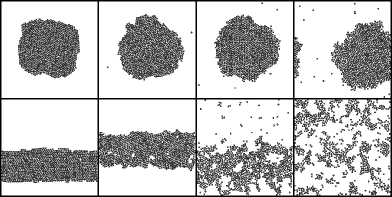
Figure 2: Typical steady–state configurations for $E=0$ (top row) and $E\rightarrow\infty$ (bottom row) at $T=$ 0.10, 0.15, 0.30 and 0.35, respectively, from left to right. This is for $N=1000$ and $\rho=0.30.$

The distribution of displacements $\vec{\delta}_{i}$ is uniform, except that the new particle position $\vec{r}_{i}^{\prime}$ is (most often in our simulations) sampled only from within the half–forward semi–circle of radius $\delta_{\text{max}}$ centered at $\vec{r}_{i},$ as illustrated in the right graph of Fig. 1. This is because the infinite–field limit, $E\rightarrow\infty,$ turns out to be most relevant, and this means, in practice, that any displacement contrary to the field is forbidden. This choice eliminates from the analysis one parameter and, more importantly, it happens to match a physically relevant case. As a matter of fact, simulations reveal that any external field $E>0$ induces a flux of particles along $\hat{x}$ —which crosses the system with toroidal boundary conditions— that monotonically increases with $E$, and eventually saturates to a maximum. This is a realistic stationary condition in which the thermal bath absorbs the excess of energy dissipated by the drive.

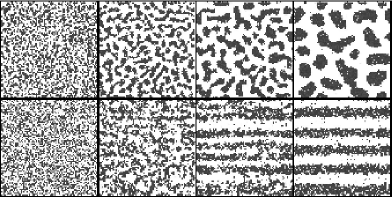
Figure 3: Typical configurations for $E=0$ (top row) and $E\rightarrow\infty$ (bottom row) as time proceeds during relaxation from a disordered state (as for $T\rightarrow\infty)$ at $t=0$. The graphs are, respectively from left to right, for times $t=$ 10${}^{2},$ 10${}^{4},$ 10${}^{5},$ and 10⁶ MC steps. This is for $N=7500$, $\rho=0.35,$ and $T=0.275,$ below the corresponding transition temperature.

III Main results

Fig. 2 illustrates late–time configurations, i.e., the ones that typically characterize the steady state, as the temperature $T$ is varied. These graphs already suggest that the system undergoes an order–disorder phase transition at some temperature $T_{E}.$ This happens to be of second order for any $E>0,$ as in the equilibrium case $E=0.$ We also observe that $T_{E}$ decreases monotonically with increasing $E,$ and that it reaches a well–defined minimum, $T_{\infty},$ as $E\rightarrow\infty.$

Fig. 2 also shows that, at low enough temperature, an anisotropic interface forms between the condensed phase and its vapor; this extends along $\hat{x}$ throughout the system at intermediate densities.

III.1 Phase segregation kinetics

Skipping microscopic details, the kinetics of phase segregation at late times looks qualitatively similar to the one in other non–equilibrium cases, including driven lattice systems hurtado and both molecular–dynamic zeng and Cahn–Hilliard ludo representations of sheared fluids, while it essentially differs from the one in the corresponding equilibrium system. This is illustrated in Fig. 3. One observes, in particular, condensation of many stripes —as in the graph for $t=10^{5}$ in Fig. 3— into a single one —as in the first three graphs at the bottom row in Fig. 2. This process corresponds to an anisotropic version of the so–called spinodal decomposition spinod , which is mainly characterized by a tendency towards minimizing the interface surface as well as by the existence of a unique relevant length, e.g., the stripe width hurtado . A detailed analysis of this late regime, which has already been studied for both equilibrium marro2 ; bray and non–equilibrium cases, including the DLG hurtado ; levine , will be the subject of a separate report.

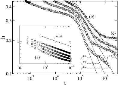
Figure 4: Time evolution of the enthalpy per particle for $N=7500,$ $\rho=0.35$ and, from top to bottom, $T=0.200,$ 0.225, 0.250 and 0.275. Straight lines are a guide to the eye; the slope of each line is indicated. The inset shows the detail at early times. (For clarity of presentation, the main graph includes a rescaling of the time corresponding to the data for $T=0.250,$ 0.225 and 0.200 by factors 2, 3 and 3, respectively.)

Detailed descriptions of early non–equilibrium nucleation are rare as compared to studies of the segregation process near completion. Following an instantaneous quench from a disordered state into $T<T_{\infty}\left(\rho\right),$ one observes in our case that small clusters form, and then some grow at the expenses of the smaller ones but rather independently of the growth of other clusters of comparable size. This corresponds to times $t<10^{5}$ in Fig. 3, i.e., before many well–defined stripes form. We monitored in this regime the excess energy or enthalpy, $H\left(t\right),$ measured as the difference between the averaged internal energy at time $t>0$ and its stationary value. This reflects more accurately the growth of the condensed droplets than its size or radius, which are difficult to be estimated during the early stages toral ; chinos . Furthermore, $H\left(t\right)$ may be determined in microcalorimetric experiments marro3 .

The time development of the enthalpy density $h\left(t\right)=H\left(t\right)/N$ is depicted in Fig. 4. This reveals some well–defined regimes at early times.

The first regime, (a) in the inset of Fig. 4, follows a power law $t^{-\theta}$ with $\theta\approx 0.165$ —which corresponds to the line shown in the graph— independently of the temperature investigated. This is the behavior predicted by the Smoluchowski coagulation or effective cluster diffusion binder2 . The same behavior was observed in computer simulations for $E=0$ and also reported to hold in actual experiments on binary mixtures toral ; marro3 . This suggests the early dominance of a rather stochastic mechanism, in which the small clusters rapidly nucleate, which is practically independent of the field, i.e., it is not affected in practice by the drive. The indication of some temperature dependence in equilibrium chinos , which is not evident here, might correspond to the distinction between deep and shallow quenches made in Ref. toral that we have not investigated out of equilibrium.

At latter times, there is a second regime, (b) in Fig. 4, in which the anisotropic clusters merge into filaments and, finally, stripes. We observe in this regime that $\theta$ varies between 0.3 and 0.6 with increasing $T$. Ostwald ripening lifshitz , consisting of monomers diffusion, predicts $\theta=1/3.$ It is likely that regime (b) describes a crossover from a situation which is dominated by monomers at low enough temperature to the emergence of other mechanisms bray ; baum which might be competing as $T$ is increased.

Finally, one observes a regime, (c) in Fig. 4, which corresponds to the beginning of spinodal decomposition.

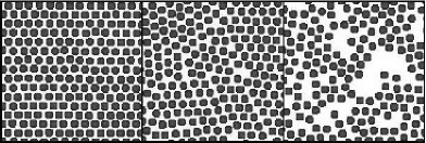
Figure 5: Details of the structure in the low$-T,$ solid phase as obtained by zooming in into configurations such as the ones in Fig. 2. This is for $T=0.05,$ $0.12$ and 0.25, from left to right, respectively.

III.2 Structure of the steady state

For any $E>0,$ the anisotropic condensate changes from a solid–like hexagonal packing of particles at low temperature (e.g., $T=0.10$ in Fig. 2), to a polycrystalline or perhaps glass–like structure with domains which show a varied morphology at (e.g.) $T=0.12.$ The latter phase further transforms, with increasing temperature, into a fluid–like structure at (e.g.) $T=0.30$ and, finally, into a disordered, gaseous state.

More specifically, the typical situation we observe at low temperature is illustrated in Fig. 5. At sufficiently low temperature, $T=0.05$ in the example, the whole condensed phase orders according to a perfect hexagon with one of its main directions along the field direction $\hat{x}.$ This is observed in approximately 90% of the configurations that we generated at $T=0.05,$ while all the hexagon axis are slanted with respect to $\hat{x}$ in the other 10% cases. As the system is heated up, the stripe looks still solid at $T=0.12$ but, as illustrated by the second graph in Fig. 5, one observes in this case several coexisting hexagonal domains with different orientations. The separation between domains is by line defects and/or vacancies. Interesting enough, as it will be shown later on, both the system energy and the particle current are practically independent of temperature up to, say $T=0.12.$ The hexagonal ordering finally disappears in the third graph of Fig. 5, which is for $T=0.25;$ this case corresponds to a fluid phase according to the criterion below.

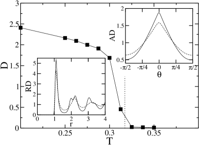
Figure 6: Data from simulations for $N=7000$ and $\rho=0.35$. The main graph shows the degree of anisotropy, as defined in the main text, versus temperature. The vertical dotted line denotes the transition temperature. The lower (upper) inset shows the radial (azimuthal) distribution at $T=0.20,$ full line, and $T=0.30,$ dashed line.

A close look to the structure is provided by the radial distribution (RD),

$$g\left(r\right)=\rho^{-2}\left\langle\sum_{i<j}\delta\left(\mathbf{r}_{i}-\mathbf{r}_{j}\right)\right\rangle,$$ (6)

i.e., the probability of finding a pair of particles a distance $r$ apart, relative to the case of a random spatial distribution at same density. This is shown in the lower inset of Fig. 6. At fixed $T,$ the driven fluid is less structured that its equilibrium counterpart, suggesting that the field favors disorder. This is already evident in Fig. 2, and it also follows from the fact that the critical temperature decreases with increasing $E.$

The essential anisotropy of the problem is revealed by the azimuthal distribution (AD) defined

$$\alpha(\theta)=N^{-2}\left\langle\sum_{i<j}\delta\left(\theta-\theta_{ij}\right)\right\rangle,$$ (7)

where $\theta_{ij}\in[0,2\pi)$ is the angle between the line connecting particles $i$ and $j$ and the field direction $\hat{x}.$ Except at equilibrium, where this is uniform, the AD is $\pi/2-$periodic with maxima at $k\pi$ and minima at $k\pi/2,$ where $k$ is an integer. The AD is depicted in the upper inset of Fig. 6.

We also monitored the degree of anisotropy, defined as the distance

$$D=\int_{0}^{2\pi}\left|\alpha-1\right|,$$ (8)

which measures the deviation from the equilibrium, isotropic case, for which $\alpha(\theta)=1,$ independent of $\theta.$ The function (8), which is depicted in the main graph of Fig. 6, reveals the existence of anisotropy even above the transition temperature. This shows the persistence of non–trivial two–point correlations at high temperatures which has been demonstrated for other non–equilibrium models pedro .

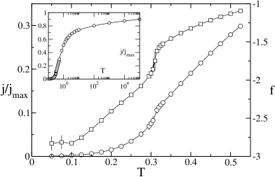
Figure 7: Temperature dependence of the mean energy (squares; the scale is on the right axis) and normalized net current (circles; scale at the left) for $N=5000$ and $\rho=0.30$ under “infinite” field. The inset shows the $T-$dependence of the current over a wider range.

III.3 Coexistence curve

The transition points may be estimated from the temperature dependence of the mean potential energy per particle,

$$f=N^{-1}\left\langle\Phi(\mathbf{\eta})\right\rangle,$$ (9)

and from the net current $j,$ defined as the mean displacement per MC step per particle. Fig. 7 shows well–defined changes of slope in both magnitudes when the phase transforms from solid to liquid ($T\approx 0.12$) and then to disorder ($T\approx 0.30$). The persistence of correlations is again revealed by the fact that the current is nonzero for any, even low $T,$ though it is small, and roughly independent of $T$, in the solid phase. The energy (9) behaves linearly with temperature for $T\in\left(0.12,0.3\right),$ as expected for a fluid phase. The maximum value of the current, $j_{max}=4\delta_{max}/3\pi,$ is only reached for $T\rightarrow\infty$. The way this limit is approached is illustrated in the inset of Fig. 7 where the grow is shown to be slower than exponential.

A main issue concerning the steady state is the liquid–vapor coexistence curve and the associated critical behavior. The (non–equilibrium) coexistence curve may be determined from the density profile transverse to the field. This is illustrated in Fig. 8.

At high enough temperature —in fact, already at $T=0.35$ in this case for which the transition temperature is slightly above 0.3— the local density is roughly constant around the mean system density, $\rho=0.35$ in Fig. 8. As $T$ is lowered, the profile accurately describes the existence of a single stripe of condensed phase of density $\rho_{+}$ which coexists with its vapor of density $\rho_{-}.$ The interface becomes thinner and smother, and $\rho_{+}$ increases while $\rho_{-}$ decreases, as $T$ is decreased.

As in equilibrium, one may use $\rho_{+}-\rho_{-}$ as an order parameter. The result of plotting $\rho_{+}$ and $\rho_{-}$ at each temperature results in the non-symmetric liquid-vapor coexistence curve shown in Fig. 9. The same result follows from the current, which in fact varies strongly correlated with the local density. Notice that the accuracy of our estimate of $\rho_{\pm}$ is favored by the existence of a linear interface. This is remarkable because we can therefore get closer to the critical point than in equilibrium. Furthermore, we found that the rectilinear diameter law,

$$\frac{1}{2}(\rho_{+}+\rho_{-})=\rho_{\infty}+b_{0}(T_{\infty}-T),$$ (10)

and the scaling law (the first term of a Wegner-type expansion wegner ),

$$\rho_{+}-\rho_{-}=a_{0}(T_{\infty}-T)^{\beta},$$ (11)

can be used here to estimate the critical parameters with higher accuracy than in the equilibrium case papa . The simulation data in Fig. 9 then yields the values in Table I, which are confirmed by the familiar log–log plots. Compared to the equilibrium critical temperature reported by Smit and Frenkel smit , one has that $T_{0}/T_{\infty}\approx 1.46,$ i.e., the change is opposite to the one for the DLG Marro . This confirms the observation above that the field acts in the non–equilibrium LJ system favoring disorder.

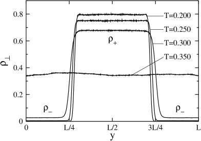
Figure 8: Density profiles transverse to the field for $N=7000,$ $\rho=0.35,$ and different temperature, as indicated. The coexisting densities, $\rho_{\pm},$ are indicated.

The fact that the order–parameter critical exponent is relatively small may already be guessed by noticing the extremely flat coexistence curve in Fig. 9. This is similar to the corresponding curve for the equilibrium two–dimensional LJ fluids smit ; 33 ; 34 , and it is fully consistent with the equilibrium Onsager value, $\beta=1/8.$ We therefore believe that our model belongs to the Ising universality class. In any case, one may discard with confidence both the DLG value $\beta\approx 1/3$ as well as the mean field value $\beta=1/2$ which was reported for fluids under shear exp —both cases would produce a hump visible to the naked eye in a plot such as the one in Fig. 9. One may argue that this result is counterintuitive, as our model apparently has the short–range interactions and symmetries that are believed to characterize the DLG.

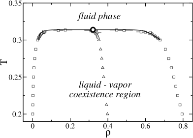
Figure 9: Coexistence curve (squares) for the LJ non-equilibrium model obtained from the density profiles in Fig. 8. The fluid phase and the coexistence region are indicated. The triangles are the arithmetic mean points, which serve to compute the critical parameters. The large circle at the top of the curve locates the critical point, and the solid line is a fit using the Wegner expansion and the rectilinear diameter law with the critical parameters given in Table I.

IV Conclusion

In summary, the present (non–equilibrium) two-dimensional Lennard–Jones system, in which particles are subject to a constant driving field, has two main general features. On one hand, this case is more convenient for computational purposses, than others such as, for instance, standard molecular–dynamics realizations of driven fluid systems. On the other, it seems to contain the necessary essential physics to be useful as a prototypical model for anisotropic behavior in nature.

This model reduces to the familiar LJ case for zero field. Otherwise, it exhibits some arresting behavior, including currents and striped patterns. We have identified two processes which seem to dominate early nucleation before anisotropic spinodal decomposition sets in. Interesting enough, they seem to be identical to the ones characterizing a similar situation in equilibrium.

We have also concluded that the model critical behavior is consistent with the Ising one for $d=2$ but not with the critical behavior of the driven lattice gas. This is puzzling. For instance, using the language of statistical field theory, symmetries seem to bring our system closer to the non–equilibrium lattice model than to the corresponding equilibrium case. The additional freedom of the present, off–lattice system, which in particular implies that the particle–hole symmetry is violated —which induces the coexistence–curve asymmetry in Fig. 9 in accordance with actual systems— are likely to matter more than suggested by some naive intuition.

Further study of the present non–equilibrium LJ system and its possible variations is suggested. A principal issue to be investigated is the apparent fact that the full non–equilibrium situations of interest can be described by some rather straightforward extension of equilibrium theory. We here report on some indications of this concerning early nucleation and properties of the coexistence curve. No doubt it would be interesting to compare more systematically the behavior of models against the varied phenomenology which was already reported for anisotropic fluids. This should also help a better understanding of non–equilibrium critical phenomena.

We acknowledge very useful discussions with M. A. Muñoz and F. de los Santos, and financial support from MEyC and FEDER (project FIS2005-00791).

References

- (1) H. Haken, Rev. Mod. Phys. 47, 67 (1975).
- (2) L. Garrido, ed., “Far from Equilibrium Phase Transitions”, Springer–Verlag, Berlin 1989.
- (3) M. C. Cross and P. C. Hohenberg, Rev. Mod. Phys. 65, 851 (1993)
- (4) J. Marro and R. Dickman, “Nonequilibrium Phase Transitions in Lattice Models” , Cambridge University Press, Cambridge 1999.
- (5) D. Beysens and M. Gbadamassi, Phys. Rev. A 22, 2250 (1980).
- (6) C.K. Chan, F. Perrot, and D. Beysens, Phys. Rev. A 43, 1826 (1991).
- (7) A. Onuki, J. Phys.: Condens. Matter 9, 6119 (1997).
- (8) R. G. Larson, “The Structure and Rheology of Complex Fluids” , Oxford University Press, New York 1999.
- (9) P. M. Reis and T. Mullin, Phys. Rev. Lett. 89, 244301 (2002).
- (10) P. Sánchez, M. R. Swift, and P. J. King, Phys. Rev. Lett. 93, 184302 (2004).
- (11) C. K. Chan, Phys. Rev. Lett. 72, 2915 (1994).
- (12) J. Dzubiella, G. P. Hoffmann, and H. Löwen, Phys. Rev. E 65, 021402 (2002).
- (13) P. I. Hurtado, J. Marro, P. L. Garrido, and E. V. Albano, Phys. Rev. B 67, 014206 (2003).
- (14) J. Hoffman, E. W. Hudson, K. M. Lang, V. Madhavan, H. Eisaki, S. Uchida, and J. C. Davis, Science, 295, 466 (2002).
- (15) J. Strempfer, I. Zegkinoglou, U. Rütt, M.v. Zimmermann, C. Bernhard, C. T. Lin, Th. Wolf, and B. Keimer, Phys. Rev. Lett. 93, 157007 (2004).
- (16) U. Zeitler, H.W. Schumacher, A.G.M. Jansen, R.J. Haug, Phys. Rev. Lett. 86, 866 (2001).
- (17) B. Spivak, Phys. Rev. B 67, 125205 (2003).
- (18) H. Yizhaq, N. J. Balmforth, and A. Provenzale, Physica D 195, 207 (2004).
- (19) B. Andreotti, Ph. Claudin, and O. Pouliquen, arXiv:cond-mat/0506758.
- (20) D.Helbing, Rev. Mod. Phys. 73, 1067 (2001).
- (21) D. Chowdhury, K. Nishinari, and A. Schadschneider, Phase Trans. 77, 601 (2004).
- (22) S.Katz, J. L. Lebowitz, and H. Spohn, J. Stat. Phys. 34, 497 (1984).
- (23) B. Schmittmann and R. K. P. Zia, in “Phase Transitions and Critical Phenomena”, Vol. 17, Academic, London 1996.
- (24) G. Ódor, Rev. Mod. Phys. 76, 663 (2004).
- (25) M. Díez–Minguito, P. L. Garrido, and J. Marro, Phys. Rev. E 72, 026103 (2005).
- (26) B. Smit and D. Frenkel, J. Chem. Phys. 94, 5663 (1991).
- (27) M. Allen and D. Tidlesley, “Computer Simulations of Liquids” , Oxford University Press, Oxford 1987.
- (28) A. Achahbar, P. L. Garrido, J. Marro, and M. A. Muñoz, Phys. Rev. Lett. 87, 195702 (2001).
- (29) E. V. Albano and G. Saracco, Phys. Rev. Lett. 88, 145701 (2002); ibid 92, 029602 (2004).
- (30) R. Yamamoto and X.C. Zeng, Phys. Rev. E 59, 3223 (1999).
- (31) L. Berthier, Phys. Rev. E 63, 051503 (2001).
- (32) K. Binder and P. Fratzl, in “Phase Transformations in Materials”, G. Kostorz ed., Wiley-VCH Verlag 2001.
- (33) J. Marro, J. L. Lebowitz, and M. H. Kalos, Phys. Rev. Lett. 43, 282 (1979).
- (34) A. Bray, Adv. Phys. 43, 357 (1994).
- (35) E. Levine, Y. Kafri, and D. Mukamel, Phys. Rev. E 64, 026105 (2001).
- (36) R. Toral and J. Marro, Phys. Rev. Lett. 54, 1424 (1985).
- (37) S. Y. Huang, X. W. Zou, and Z. Z. Jin, J. Phys.: Condens. Matter 13, 7343 (2001).
- (38) J. Marro, R. Toral, and A. M. Zahra, J. Phys. C 18, 1377 (1985).
- (39) K. Binder and D. Stauffer, Phys. Rev. Lett. 33, 1006 (1974).
- (40) W. Ostwald, Z. Phys. Chem. 37, 385 (1901); I. Lifshitz and V. Slyozov, J. Phys. Chem. Solids 19, 35 (1961); C. Wagner, Z. Elektrochem. 65, 58 (1961).
- (41) T. Baumberger, F. Perrot, and D. Beysens, Phys. Rev. A 46, 7636 (1992).
- (42) P. L. Garrido, J. L. Lebowitz, C. Maes, and H. Spohn, Phys. Rev. A 42, 1954 (1990).
- (43) F. Wegner, Phys. Rev. B 5, 4529 (1972).
- (44) This is in spite of the fact that these fits, and the so–called MC Gibbs method, which are widely used for fluids in thermal equilibrium because of its accuracy when estimating coexistence–curve properties Pana0 , have no justification out of equilibrium.
- (45) A.Z. Panagiotopopoulos, Molecular Phys. 61, 813 (1987).
- (46) R.R. Singh, K. S. Pitzer, J. J. de Pablo, and J. M. Pravsnitz, J. Chem. Phys. 92, 5463 (1990).
- (47) A.Z. Panagiotopopoulos, Int. J. Thermophys. 15, 1057 (1994)
0.321(5) 0.314(1) 0.10(8)
TABLE I: Critical indexes