Universality classes of the Kardar-Parisi-Zhang equation

Abstract

We re-examine mode-coupling theory for the Kardar-Parisi-Zhang (KPZ) equation in the strong coupling limit and show that there exists two branches of solutions. One branch (or universality class) only exists for dimensionalities $d<d_{c}=2$ and is similar to that found by a variety of analytic approaches, including replica symmetry breaking and Flory-Imry-Ma arguments. The second branch exists up to $d_{c}=4$ and gives values for the dynamical exponent $z$ similar to those of numerical studies for $d\geq 2$.

The celebrated Kardar-Parisi-Zhang (KPZ) equation kardar86 was initially derived as a model to describe the kinetic roughening of a growing interface and has been the subject of a great number of theoretical studies halpin95 . This is because the original growth problem has turned out to be equivalent to other important physical phenomena, such as the randomly stirred fluid (Burgers equation) forster77 , directed polymers in random media (DPRM) kardar87 , dissipative transport beijeren85 ; janssen86 or magnetic flux lines in superconductors hwa92 . The KPZ equation has thus emerged as one of the fundamental theoretical models for the study of universality classes in non-equilibrium scaling phenomena and phase transitions halpin95 .

It is a non-linear Langevin equation which describes the large-distance, long-time dynamics of the growth process specified by a single-valued height function $h({\bf x},t)$ on a $d$-dimensional substrate ${\bf x}\in\mathrm{I\!R}^{d}$:

$$\partial_{t}h({\bf x},t)=\nu\,\nabla^{2}h({\bf x},t)\,+\,\lambda/2\,\big{(}\nabla h({\bf x},t)\big{)}^{2}\,+\,\eta({\bf x},t),$$ (1)

where $\eta({\bf x},t)$ is a zero mean uncorrelated noise with variance $\langle\eta({\bf x},t)\eta({\bf x}^{\prime},t^{\prime})\rangle=2D\delta^{d}({\bf x}-{\bf x}^{\prime})\,\delta(t-t^{\prime})$. This equation reflects the competition between the surface tension smoothing force $\nu\nabla^{2}h$, the preferential growth along the local normal to the surface represented by the non-linear term and the Langevin noise $\eta$ which tends to roughen the interface and mimics the stochastic nature of the growth.

The stationary interface is characterized by the two-point correlation function $C(|{\bf x}-{\bf x}^{\prime}|,t-t^{\prime})\equiv\langle[h({\bf x},t)-h({\bf x}^{\prime},t^{\prime})]^{2}\rangle$ and, in particular, its large-scale properties where $C$ is expected to assume the scaling form $C(d,\tau)=d^{2\chi}\,f(\frac{\tau}{d^{z}})$, where $d=|{\bf x}-{\bf x}^{\prime}|$ , $\tau=|t-t^{\prime}|$ and $\chi$ and $z$ are the roughness and dynamical exponents respectively. These two exponents are not independent since the Galilean symmetry forster77 — the invariance of Eq. (1) under an infinitesimal tilting of the interface — enforces the scaling relation $z+\chi=2$ for solutions associated with any fixed point at which $\lambda$ is non-zero.

While some exact results are available in $d=1$, yielding $\chi=1/2$ and $z=3/2$ kardar87 ; hwa91 ; halpin95 , the complete theoretical understanding of the KPZ equation in higher dimensions is still lacking. For $d>2$, there exists a phase transition between two different regimes, separated by a critical value $\lambda_{c}$ of the non-linear coefficient kardar86 ; forster77 . In the weak-coupling regime ($\lambda<\lambda_{c}$), the behavior is governed by the $\lambda=0$ fixed point — corresponding to the linear Edwards-Wilkinson equation halpin95 — with exponents $\chi=(2-d)/d$ and $z=2$. In the strong-coupling (rough) regime ($\lambda>\lambda_{c}$), the non-linearity becomes relevant and despite considerable efforts, the statistical properties of the strong-coupling (rough) regime for $d\geq 2$ remain controversial.

The existence of a finite upper critical dimension $d_{c}$ at which the dynamical exponent $z$ of the strong-coupling phase becomes 2 is also much debated. Most of the analytical approaches support a finite $d_{c}$, but their predictions are varied: one of the solutions of the mode-coupling (MC) equations and other arguments indicate $d_{c}\simeq 4$ bouchaud93 ; halpin89 ; colaiori01 ; colaiori01b , whereas functional renormalization group to two-loop order suggests $d_{c}\simeq 2.5$ ledoussal03 . A set of related theories such as replica symmetry breaking MP , variational studies GO and Flory-Imry-Ma arguments MG give $d_{c}=2$. On the other hand, numerical simulations and real space calculations find no evidence at all for a finite $d_{c}$ tang92 ; marinari00 ; castellano98 !

We re-examine in this paper MC theory. It is a self-consistent approximation beijeren85 ; janssen86 , where in the diagrammatic expansion for the correlation and response functions only diagrams which do not renormalize the three-point vertex $\lambda$ are retained. The MC approximation has been widely studied hwa91 ; frey96 ; bouchaud93 ; doherty94 ; colaiori01 . Furthermore the MC equations are exact for the large $N$-limit of a generalised $N$-component KPZ doherty94 . This allows in principle for a systematic expansion in $1/N$. We shall show that within the MC approximation there exists two solutions, one of which had been previously overlooked. The new solution (universality class) only exists when $d<2$ and seems similar to the solution found in the analytical studies which give $d_{c}=2$ MP ; GO ; MG . The other MC solution exists on the whole range $0<d<4$ and has $d_{c}=4$. This previously known solution gives in $d=2$ a value for $z$ close to that from numerical work, e.g. marinari00 .

The correlation and response functions are defined in Fourier space by $C({k},\omega)=\langle h({k},\omega)h^{*}({k},\omega)\rangle$ and $G({k},\omega)\delta^{d}({k}-{k^{\prime}})\delta(\omega-\omega^{\prime})=\Big{\langle}\displaystyle\frac{\partial h({k},\omega)}{\partial\eta({k^{\prime}},\omega^{\prime})}\Big{\rangle}$, where $\langle\cdot\rangle$ indicates an average over $\eta$. In the MC approximation, the correlation and response functions are the solutions of two coupled equations,

$$G^{-1}({k},\omega) = G^{-1}_{0}({k},\omega)+\lambda^{2}\displaystyle\int\displaystyle\frac{d\Omega}{2\pi}\displaystyle\int\displaystyle\frac{d^{d}q}{(2\pi)^{d}}\,{q}\cdot({k}-{q})$$ (2)

$$\times \left({q}\cdot{k}\right)G({k}-{q},\omega-\Omega)\,C({q},\Omega)$$

$$C({k},\omega) = C_{0}({k},\omega)+\displaystyle\frac{\lambda^{2}}{2}\big{|}G({k},\omega)\big{|}^{2}\displaystyle\int\displaystyle\frac{d\Omega}{2\pi}\displaystyle\int\displaystyle\frac{d^{d}q}{(2\pi)^{d}}$$ (3)

$$\times \left({q}\cdot({k}-{q})\right)^{2}C({k}-{q},\omega-\Omega)\,C({q},\Omega)$$

where $G_{0}({k},\omega)=(\nu k^{2}-i\omega)^{-1}$ is the bare response function, and $C_{0}({k},\omega)=2D|G({k},\omega)|^{2}$ bouchaud93 . In the scaling limit, $G({k},\omega)$ and $C({k},\omega)$ take the forms $G({k},\omega)=k^{-z}g\left(\omega/k^{z}\right)$ and $C({k},\omega)=k^{-(2\chi+d+z)}n\left(\omega/k^{z}\right)$ and Eqs. (2) and (3) translate into coupled equations for the scaling functions $n(x)$ and $g(x)$:

$$g^{-1}(x) = -ix+I_{1}(x)\,,$$ (4)

$$n(x) = |g(x)|^{2}I_{2}(x)\,,$$ (5)

where $x=\omega/k^{z}$ and $I_{1}(x)$ and $I_{2}(x)$ are given by bouchaud93

$$I_{1}(x) = P\displaystyle\int_{0}^{\pi}d\theta\sin^{d-2}\theta\displaystyle\int_{0}^{\infty}dq\cos\theta(\cos\theta-q)$$

$$\times q^{2z-3}r^{-z}\displaystyle\int_{-\infty}^{\infty}dy\,g\left(\displaystyle\frac{x-q^{z}y}{r^{z}}\right)n(y),$$

$$I_{2}(x) = \displaystyle\frac{P}{2}\displaystyle\int_{0}^{\pi}d\theta\sin^{d-2}\theta\displaystyle\int_{0}^{\infty}dq(\cos\theta-q)^{2}$$

$$\times q^{2z-3}r^{-(d+4-z)}\displaystyle\int_{-\infty}^{\infty}dy\,n\left(\displaystyle\frac{x-q^{z}y}{r^{z}}\right)n(y),$$

with $P\!=\!\lambda^{2}/(2^{d}\Gamma(\frac{d-1}{2})\pi^{(d+3)/2})$, $r^{2}=1+q^{2}-2q\cos\theta$. Notice that the “bare term” $C_{0}({k},\omega)$ has been dropped from these equations as it is negligible in the scaling limit provided $2\chi+d+z>2z$, i.e. $4+d>3z$.

All the (necessarily approximate) solutions of the MC equations involve an ansatz on the form of the scaling functions $n(x)$ and $g(x)$. The relation $z=z(d)$ is then obtained requiring consistency of Eqs. (4) and (5) on matching both sides at an arbitrarily chosen value of $x$. Due to the non-locality of Eqs. (4) and (5), the matching condition depends on the form of the functions $n$ and $g$ for all $x$, so the ansatz needs to be reliable for all $x$, and in particular satisfy the large $x$ asymptotic forms $n(x)\sim x^{-1-\beta/z}$, $g_{R}(x)\sim x^{-1-2/z}$ and $g_{I}(x)\rightarrow x^{-1}$ where $\beta=d+4-2z$ and $g(x)=g_{R}(x)+ig_{I}(x)$. Colaiori and Moore colaiori01 ; colaiori01b proposed an ansatz which satisfies these large $x$ constraints. It enabled the authors to provide numerical estimates of $z$ when $d=2,3$ in reasonable agreement with exponents obtained from simulations marinari00 ; tang92 . It also yielded an integer finite upper critical dimension $d_{c}=4$ colaiori01 . Moreover, it led in $d=1$ to the discovery of a stretched exponential behavior for the two-point correlation function colaiori01b similar to that found in the exact solution PS04 .

Using a similar ansatz, we next show that Eqs. (4) and (5) have an additional solution with $d_{c}=2$, before discussing its significance. The advocated ansatz is most conveniently expressed in Fourier space,

$$\widehat{g}(p) = \theta(p)\,\exp(-|p|^{2/z})\,,$$ (6)

$$\widehat{n}(p) = A\exp(-\displaystyle\big{|}Bp\big{|}^{\beta/z})\,,$$ (7)

where $\widehat{n}$ and $\widehat{g}$ are the Fourier transform of $n(x)$ and $g(x)$ respectively, $A$ is a (nonzero) parameter and $B\equiv B(d,z)$ an arbitrary function colaiori01 . Requiring the matching of Eqs. (4) and (5) at large $x$ then yields:

$${C_{d}\,A}\,{B}^{-1} = {d\,(2-z)}/{(z^{2}\,I(B,d,z))}$$ (8)

$${C_{d}\,A}\,{B^{-2}} = (\beta/z)^{2}\,(\beta-z)\,{2^{\frac{2z-\beta}{\beta}}}/{\Gamma\big{(}\frac{2z-\beta}{\beta}\big{)}}$$ (9)

where $C_{d}=\lambda^{2}\,\Gamma((d-1)/2)/(4\,\pi^{\frac{d+1}{2}}\,\Gamma(d-1))$ and $I(B,d,z)\!=\!\displaystyle\int_{0}^{\infty}\!ds\,B\,(1-2s^{2})s^{2z-3}\exp\big{(}-B^{\beta/z}s^{\beta}-s^{2}\big{)}$. Combining (8) and (9) then gives an implicit equation for the curve $z(d)$ depending on $B$ only:

$$\beta^{2}\,(\beta-z)\,\frac{2^{(2z-\beta)/\beta}}{\Gamma\big{(}\frac{2z-\beta}{\beta}\big{)}}\,I(B,d,z)=\frac{d\,(2-z)}{B}.$$ (10)

Eq. (10) can be solved numerically once $B(d,z)$ has been fixed. Prior to discussing the choice of $B$, we stress the ($B$-independent) intrinsic properties of the solutions $S_{d,z}$. First, as $z\to 2$, $I(B,d,2)$ is finite for any $B>0$. One can then infer from Eq. (10) that $S_{2,2}$ and $S_{4,2}$ are always solutions independent of $B$ (provided $B^{-1}$ is finite). This singles out the two dimensions $d_{c}=2$ and $d_{c}=4$ as critical ones since $z\to 2$ for $d\to d_{c}$. Second, as $d\to 0$, $I(B,0,z)$ is non-zero for any $B>0$, and Eq. (10) yields the two solutions $S_{0,4/3}$ and $S_{0,1}$ (provided again $B^{-1}$ is finite). Lastly, as the MC equations satisfy the fluctuation-dissipation theorem (FDT) that exists in $d=1$ frey96 yielding the exact result $z=3/2$, we expect the ansatz to preserve this property, which is fulfilled for $B(1,3/2)=1$ as can be checked on Eqs. (6) and (7). It follows that $S_{1,3/2}$ is solution of (10). To summarize, Eq. (10) has five intrinsic solutions $S_{d,z}$ which do not depend on the choice of $B$ (provided $B^{-1}<\infty$ and $B(1,3/2)~{}=~{}1$).

Furthermore, Eq. (8) provides additional constraints on $B(d,z)$ in the two limits $z\to 2$ and $d\to 0$. As $I(B,d,2)$ is finite as $z\to 2$, the right-hand side of (8) vanishes identically, which forces $B^{-1}\sim(2-z)$ on the left-hand side. One can then derive the expansions of two solutions, labelled $z_{\rm S}$ and $z_{\rm F}$, about their critical dimensions:

$$z_{\rm F} = 2-(4-d)/4+{\cal O}((4-d)^{2})$$ (11)

$$z_{\rm S} = 2-(2-d)/3+{\cal O}((2-d)^{2}).$$ (12)

The arguments of Ref. colaiori01 can be used to show that these expansions are very robust and more general than the particular ansatz of Eqs. (6) and (7). Similarly, as $I(B,0,z)$ is finite for $d\to 0$ and $z>1$, Eq. (8) imposes $B^{-1}\sim d$. The expansions of the two solutions about $d=0$ can also be worked out: $z_{\rm F}=4/3+d/3+{\cal O}(d^{2})$ and $z_{\rm S}=1+d/4+{\cal O}(d^{2})$.

We emphasize that all these features do not depend on the choice of $B$. Any ansatz would lead to the same qualitative picture as Fig. 1 provided $B\sim(d(2-z))^{-1}$. The specific one used here further exploits the uniqueness of the solution in $d=1$ which imposes additional constraints on $B$ . With this choice, we have solved Eq. (10) numerically in $0<d<4$ and found that there exists two branches of solutions $z_{\rm S}(d)$ and $z_{\rm F}(d)$ lying in the interval $d\in(0,2)$ but only one solution, the continuation of $z_{\rm F}$, in the interval $d\in(2,4)$.

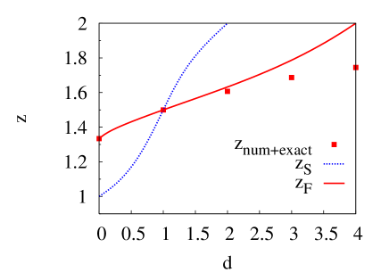
Figure 1: The two solutions $z_{\rm S}(d)$ and $z_{\rm F}(d)$ of the MC equations found in this work, compared with numerical marinari00 results for $d=2,3,4$ and the exact results in $d=0,1$, all represented by squares.

The branch $z_{\rm F}$, referred to as the F solution as it exists over the full dimensionality range $d\in(0,4)$, is similar to the solution analyzed in colaiori01 . It lies fairly close to typical numerical results marinari00 with $z=1.632$ for $d=2$ and $z=1.787$ for $d=3$, reproduces the exact results in $d=0$ and $d=1$ (see Fig. 1) and reaches $z=2$ at $d_{c}=4$, which defines the upper critical dimension of this solution. The other branch, denoted S as it is associated with the shorter dimensionality interval $d\in(0,2)$, embodies a new universality class with $z_{\rm S}\neq z_{\rm F}$ for $d\neq 1$. For this solution, $z=2$ at $d_{c}=2$ and it does not exist for $d\geq 2$, so that there remains a single strong-coupling solution in and above two dimensions – the F solution. We emphasise that both the F and S solutions are non-perturbative since no (stable) perturbative fixed point can be found for $d<2$ within the standard perturbative expansion in the coupling constant $g={2\lambda^{2}D}/{\nu^{3}}$, even to all orders Wiese . MC theory involves resumming an infinite set of diagrams and so is capable of going beyond standard RG techniques.

We now comment on our findings. According to MC theory, for $d<2$ there are two possible strong-coupling universality classes, F and S. It is clear that for a given set of initial conditions and bare correlators, the time evolution would unambiguously steer the system towards one or other of the two solutions. Equivalently, in the mapping to the DPRM, the solution with lowest free energy would be selected as the physical one. The apparent freedom to choose a solution arises because we have considered the scaling regime in which the bare correlators have been dropped as irrelevant, so we have lost track of their role. However, a clue as to the form of bare correlator needed for the S solution to emerge can be obtained by inspecting the zero-dimensional case. In $d=0$, the DPRM analogue is a directed walk along a chain of length $L$ on which the site energies are random. A dynamical exponent $z=1$ would correspond to free energy fluctuations of order $L^{2/z-1}=L$ which is larger than the $\sqrt{L}$ (for $z=4/3$) expected for independent random site energies. with $z=1$ could only exist with long-range correlations between the site energies and is therefore not the natural solution for the short-range problem in $d=0$. We suspect that the $z_{\rm S}$ branch in the whole range $0<d<2$ would only be realized if there were some long-range correlations in the noise for the KPZ problem or between the site energies for the DPRM analogue.

To investigate this possibility further, suppose instead of starting out with noise with short-range correlations, one introduces some long-ranged correlated noise, of the form $\langle\eta({x},t)\eta({x^{\prime}},t^{\prime})\rangle=2R({x}-{x^{\prime}})\delta(t-t^{\prime})$ with some power law distribution $R({x})\propto x^{2\rho-d}$, or equivalently in Fourier space $R({k})=D(1+wk^{-2\rho})$. The MC equations would formally be the same with $D$ replaced by the ‘generalized’ noise correlator $R({k})$ frey96 . These long-range bare noise correlations will not affect the scaling behavior of the system as long as they decay sufficiently quickly, so that they become irrelevant after some transient regime. The condition for this to happen can be worked out by substituting the scaling forms for $G$ and $C$ into Eq. (3). The initial correlations decay as $C_{0}({k},\omega)=2R({k})|G({k},\omega)|^{2}\sim k^{-2(z+\rho)}$ whereas the long-time correlation function is expected to behave as $C({k},\omega)\sim k^{-(2\chi+d+z)}\equiv k^{-(d+4-z)}$ using the identity $z+\chi=2$. Comparing these two expressions, one infers that the long-range correlations will destabilize a short-range solution with dynamical exponent $z$ when

$$\rho>\frac{d+4-3z}{2},$$ (13)

which is identical to the criterion obtained in frey99 from RG arguments. The condition of Eq. (13) determines the phase boundary $\rho(d,z)$ between the short-range and long-range stability domains for each of the two MC solutions $z_{\rm F}$ and $z_{\rm S}$. In the long-range noise dominated region $z_{\rm LR}=\frac{d+4-2\rho}{3}$ frey99 . The solutions F and S are stable against noise of range $\rho$ if their associated $z$ satisfies $z<z_{\rm LR}$. For all $0<d<2$, we believe that the S solution requires for its existence the addition of long-range noise of infinitesimal amplitude with $\rho_{S}=\frac{d+4-3z_{\rm S}}{2}$, as in the case $d=0$ (where $z=1$ would correspond to long-range noise with $\rho=0.5^{-}$). For $0<d<1$, the S solution lies at the stability limit of the long-range solution and in the interval $1<d<2$, it will be the solution to the KPZ problem in the presence of infinitesimal amounts of such correlated noise if (say) the associated free energy in the DPRM analogue is lower than that of the F solution (with the same correlated noise). This S solution could hence possibly be brought out by tuning the parameters. We believe that in the absence of some long-range correlation, the F solution will be the appropriate solution or universality class for $0<d<4$.

Our S solution might appear to be of academic interest as it only exists when $d<2$ and coincides with the F one in $d=1$. However, it turns out to be strikingly similar to the solution found in several theoretical studies. We focus on three of them: the replica symmetry breaking (RSB) calculation of Mézard and Parisi MP , a Gaussian variational calculation GO and Flory-Imry-Ma (FIM) arguments MG . All three approaches result in a strong-coupling solution with $d_{c}=2$. The RSB treatment yields a dynamical exponent equivalent to the FIM result MP : $z_{\rm FIM}=(4+d)/3\simeq 2-(2-d)/3+{\cal O}((2-d)^{2})$, which is identical to (12) and suggests that the MC solution S and the RSB – FIM solution are indeed different approximations to the same underlying universality class. It is not apparent how the long-range correlations needed for the S solution to exist enter these analytical approaches. However, it has been observed long ago that by the addition of a type of long-range force, the Flory formula in the conventional self-avoiding polymer problem becomes exact MB .

To summarize, we have found a new MC solution, S, which has an upper critical dimension $d_{c}=2$, in addition to the usual one, F, which has $d_{c}=4$. This new solution seems similar to that found by analytical treatments such as RSB and FIM arguments, but we believe will only exist in the presence of appropriate long-range correlated noise. We acknowledge that the numerical value for $z$ shown in Fig. 1 when $d=4$ is not apparently consistent with the upper critical dimension $d_{c}=4$ of the F solution, but we attribute that to the inability of numerical studies in high dimensions to access the scaling regime.

- (1) M. Kardar, G. Parisi, and Y.-C. Zhang, Phys. Rev. Lett. 56, 889 (1986).
- (2) T. Halpin-Healy and Y. Zhang, Phys. Rep. 245, 218 (1995), J. Krug, Adv. Phys. 46, 139 (1997).
- (3) D. Forster, D. R. Nelson, and M. J. Stephen, Phys. Rev. A 16, 732 (1977).
- (4) M. Kardar, Nucl. Phys. B 290, 582 (1987).
- (5) H. van Beijeren, R. Kutner, and H. Spohn, Phys. Rev. Lett. 54, 2026 (1985).
- (6) H. K. Janssen and B. Schmittmann, Z. Phys. B 63, 517 (1986).
- (7) T. Hwa, Phys. Rev. Lett. 69, 1552 (1992).
- (8) T. Hwa and E. Frey, Phys. Rev. A 44, R7873 (1991).
- (9) M. A. Moore et al., Phys. Rev. Lett. 74, 4257 (1995), J.-P. Bouchaud and M. E. Cates, Phys. Rev. E 47, R1455 (1993)
- (10) T. Halpin-Healy, Phys. Rev. Lett. 62, 442 (1989), H. C. Fogedby, Phys. Rev. Lett. 94, 195702 (2005).
- (11) F. Colaiori and M. A. Moore, Phys. Rev. Lett. 86, 3946 (2001).
- (12) F. Colaiori and M. A. Moore, Phys. Rev. E 63, 057103 (2001), Phys. Rev. E 65, 017105 (2001).
- (13) P. Le Doussal and K. J. Wiese, Phys. Rev. B 68, 174202 (2003), Phys. Rev. E 72, 035101(R) (2005).
- (14) M. Mézard and G. Parisi, J. Phys. I,1, 809 (1991).
- (15) T. Garel and H. Orland, Phys. Rev. B 55, 226 (1997).
- (16) C. Monthus and T. Garel, Phys. Rev. E 69, 061112 (2004).
- (17) L.-H. Tang, B. M. Forrest, and D. E. Wolf, Phys. Rev. A 45, 7162 (1992), T. Ala-Nissila, T. Hjelt, J. M. Kosterlitz, and O. Venäläinen, J. Stat. Phys. 72, 207 (1993), E. Marinari, A. Pagnani, G. Parisi, and Z. Rácz, Phys. Rev. E 65, 026136/1 (2002).
- (18) E. Marinari, A. Pagnani, and G. Parisi, J. Phys. A 33, 8181 (2000).
- (19) C. Castellano, M. Marsili, and L. Pietronero, Phys. Rev. Lett. 80, 3527 (1998), C. Castellano, M. Marsili, M. A. Muñoz, and L. Pietronero, Phys. Rev. E 59, 6460 (1999).
- (20) J. P. Doherty, M. A. Moore, J. M. Kim, and A. J. Bray, Phys. Rev. Lett. 72, 2041 (1994).
- (21) E. Frey, U. C. Täuber, and T. Hwa, Phys. Rev. E 53, 4424 (1996).
- (22) M. Prähofer and H. Spohn, J. Stat. Phys. 115, 255 (2004).
- (23) K. J. Wiese, J. Stat. Phys. 93, 143 (1998).
- (24) E. Frey, U. C. Täuber, and H. K. Janssen, Europhys. Lett. 47, 14, 1999.
- (25) M. A. Moore and A. J. Bray, J. Phys. A: Math. Gen. 11, 1353 (1978), Y. Chen and R. A. Guyer J. Phys. A: Math. Gen. 21, 4173 (1988).