Supramolecule Structure for Amphiphilic Molecule
by Dissipative Particle Dynamics Simulation

Hiroaki NAKAMURA

Theory and Computer Simulation Center / The Graduate University for Advanced Studies, National Institute for Fusion Science, 322-6 Oroshi-cho, Toki, Gifu 509-5292, JAPAN (Received )

Meso-scale simulation of structure formation for AB-dimers in solution W monomers was performed by dissipative particle dynamics (DPD) algorithm. As a simulation model, modified Jury Model was adopted [Jury, S. et al. “Simulation of amphiphilic mesophases using dissipative particle dynamics,” Phys. Chem. Chem. Phys. 1 (1999) 2051–2056], which represents mechanics of self-assembly for surfactant hexaethylene glycol dodecyl ether (${\rm C}_{12}{\rm E}_{6}$) and water(${\rm H}_{2}$O). The same phase diagram as Jury’s result was obtained. We also found that it takes a longer time to form the hexagonal phase (${\rm H}_{1}$) than to form the lamellar phase (${\rm L}_{\alpha})$.

Keywords: Amphiphilic molecule, Nonionic surfactant, Dissipative particle dynamics simulation, Self assembly, Structure formation, Phase diagram

INTRODUCTION

Dissipative particle dynamics (DPD) simulation has become one of the most powerful algorithm for soft-matter research[1, 2, 3, 4]. In DPD simulation, the conservative interaction potentials are soft-repulsive, which make simulation of long-time phenomena possible. By the way, DPD algorithm might be considered one of the coarse-grained method of molecular dynamics(MD) simulation. Some information of interaction potential between particles are neglected and simplified. We, therefore, must pick up the dominant interaction potential for the mesoscopic structure formation. Because we don’t have enough experimental data for the interaction potentials, it becomes a difficult problem of DPD simulation how we define interaction parameters. In 1999, Jury et al. succeeded, by an empirical method, the DPD simulation of the smectic mesophase for a simple amphiphilic molecule system with water solvent [5]. They showed that their minimal model (we call it Jury model), which is composed of rigid AB dimers in solution W monomers, is very proper to present phase diagram of surfactant hexaethylene glycol dodecyl ether (${\rm C}_{12}{\rm E}_{6}$) and water (${\rm H}_{2}{\rm O}$)[5, 6]. In this paper, we reveal processes of self-organization of one smectic mesophase by modified Jury model which has such a difference from the original Jury model that attractive harmonic oscillator potential is used as a covalent bond potential between A and B particles in the same molecule. Details of simulation method are explained in the next section. In the last section, we will show such a interesting property of the system that it take a longer time to form the hexagonal phase (${\rm H}_{1}$) than the lamellar phase $({\rm L}_{\alpha})$ which is more symmetric than ${\rm H}_{1}$ phase. It is considered intuitively that it takes a longer time to form the higher ordered phase than to form the lower ordered phase. However, this simulation shows that it takes a longer time to form the lower ordered phase than to form the higher ordered phase contrary to the intuitive consideration.

SIMULATION METHOD

DPD Algorithm

First of all, we express the DPD model and algorithm[2, 5]. According to ordinarily DPD model, all atoms are coarse-grained to particles whose mass are the same one. We define the total number of particles as $N.$ The position and velocity vectors of particle $i,(i=1,\cdots,N),$ are indicated by $\mbox{\boldmath$r$}_{i}$ and $\mbox{\boldmath$v$}_{i}$, respectively. The particle $i$ moves according to the following equation of motion, where all physical quantities are made dimensionless to handle easily in actual simulation.

$$\frac{d\mbox{\boldmath$r$}_{i}}{dt} = \mbox{\boldmath$v$}_{i},$$ (1)

$$\frac{d\mbox{\boldmath$v$}_{i}}{dt} = \sum_{j(\neq i)}^{N}\mbox{\boldmath$F$}_{ij},$$ (2)

where a particle $i$ interacts with the other particle $j$ by $\mbox{\boldmath$F$}_{ij}$ is the total force

$$\mbox{\boldmath$F$}_{ij}=\mbox{\boldmath$F$}_{ij}^{\rm C}+\mbox{\boldmath$F$}_{ij}^{\rm R}+\mbox{\boldmath$F$}_{ij}^{\rm D}+\mbox{\boldmath$F$}_{ij}^{\rm B}.$$ (3)

In Eq. 3, $\mbox{\boldmath$F$}^{\rm C}_{ij}$ is a conservative force deriving from a potential exerted on particle $i$ by the $j-$particle, $\mbox{\boldmath$F$}^{\rm D}_{ij}$ and $\mbox{\boldmath$F$}^{\rm R}_{ij}$ are the dissipative and random forces between particle $i$ and $j$, respectively. Furthermore, neighboring particles on the same amphiphilic molecule are bound by the bond-stretching force $\mbox{\boldmath$F$}^{\rm B}_{ij}$.

The conservative force $\mbox{\boldmath$F$}^{\rm C}$ has the following form:

$$\mbox{\boldmath$F$}^{\rm C}_{ij}=-\nabla_{i}\phi_{ij},$$ (4)

where $\nabla_{i}\equiv\partial/\partial\mbox{\boldmath$r$}_{i}$. For computational convenience, we adopted that the cut-off length as the unit of length. It is assumed that the conservative force $\mbox{\boldmath$F$}^{\rm C}$ are truncated at this radius. Following this assumption, the two-point potential $\phi_{ij}$ in Eq. 4 is defined as follows:

$$\phi_{ij}\equiv\phi(r_{ij})=\frac{1}{2}a_{ij}\left(r_{ij}-1\right)^{2}H(1-r_{ij}),$$ (5)

where $r_{ij}=|\mbox{\boldmath$r$}_{ij}|;\mbox{\boldmath$r$}_{ij}\equiv\mbox{\boldmath$r$}_{j}-\mbox{\boldmath$r$}_{i}$. We also define the unit vector $\mbox{\boldmath$n$}_{ij}\equiv\mbox{\boldmath$r$}_{ij}/r_{ij}$ between particles $i$ and $j$. The Heaviside step function $H$ in Eq. 5 is defined by

$$H(x)\equiv\left\{\begin{array}[]{ll}0&\mbox{ for }\ \ x<0,\\ \frac{1}{2}&\mbox{ at }\ \ x=0,\\ 1&\mbox{ for }\ \ x>0.\end{array}\right.$$ (6)

Español and Warren proposed that the following simple form of the random and dissipative forces, as follows[7]:

$${\mbox{\boldmath$F$}}_{ij}^{\rm R} = \sigma\omega_{\rm R}(r_{ij})\mbox{\boldmath$n$}_{ij}\frac{\zeta_{ij}}{\sqrt{\Delta t}},$$ (7)

$${\mbox{\boldmath$F$}}_{ij}^{\rm D} = -\gamma\omega_{\rm D}(r_{ij})\left(\mbox{\boldmath$v$}_{ij}\cdot\mbox{\boldmath$n$}_{i,j}\right)\mbox{\boldmath$n$}_{ij},$$ (8)

where $\zeta_{ij}$ is a Gaussian random valuable with zero mean and unit variance, chosen independently for each pair $(i,j)$ of interacting particles at each time-step and $\zeta_{ij}=\zeta_{ji}.$ The strength of the dissipative and random forces is determined by the dimensionless parameter $\sigma$ and $\gamma$, respectively. The parameter $\Delta t$ is a dimensionless time-interval of integrating the equation of motion.

Now we consider the fluctuation-dissipative theorem of DPD method. The time evolution of the distribution function of the DPD system is governed by Fokker-Planck equation[7]. The system evolves to the same steady state as the Hamiltonian system, that is, Gibbs-Boltzmann canonical ensemble, if the coefficients of the diffusion and random force terms have the following relations:

$$\omega_{\rm D} = \left(\omega_{\rm R}\right)^{2},$$ (9)

$$\sigma^{2} = 2T\gamma,$$ (10)

where $T$ is the dimensionless equilibrium-temperature. The forms of the weight functions $\omega_{\rm D}$ and $\omega_{\rm R}$ are not specified by the original DPD algorithm. We adopted the following simple form as the weighting functions[7]:

$$\omega_{\rm R}(r)=\left\{\omega_{\rm D}(r)\right\}^{1/2}=\omega\left(r\right).$$ (11)

Here the function $\omega$ is defined by[7, 2].

$$\omega(x)\equiv(1-x)H(1-x).$$ (12)

$a_{ij}$	W	A	B
W	25	0	50
A	0	25	30
B	50	30	25

Table 1: The table of the coefficients $a_{ij}$, which depend on kinds of particles $i$ and $j$; W is a “water” particle, A is a “hydrophilic” particle and B is a “hydrophobic” one.

Finally, we use the following form as the bond-stretching force:

$$\mbox{\boldmath$F$}_{ij}^{\rm B}=-\nabla_{i}\phi_{ij}^{\rm B},$$ (13)

where $\phi_{\rm B}$ is the dimensionless bond-stretching potential energy. When particles $i$ and $j$ are connected in the same molecule, they interact with each others by the following potential energy:

$$\phi_{ij}^{\rm B}\equiv\phi^{\rm B}(r_{ij})=\frac{1}{2}a_{\rm B}r_{ij}^{2},\mbox{ \ \ \ if $i$ is connected to $j$.}$$ (14)

Here $a_{\rm B}$ is the potential energy coefficient and $r_{0}$ is the equilibrium bond length.

Simulation Model and Parameters

As the model, we used modified Jury model molecule to dimer which is composed of hydrophilic particle (A) and hydrophobic one (B)[5]. Water molecules are also modeled to coarse-grained particles W. All mass of particles are assumed to unity. The number density of particle $\rho$ is set to $\rho=6$. The number of modeled amphiphilic molecules AB is shown as $N_{\rm AB}$, the number of water $N_{\rm W}.$ Total number of particle $N\equiv 2N_{\rm AB}+N_{\rm W}$ is fixed to $N=10000.$ The simulation box is set to cubic. The dimensionless length of the box $L$ is

$$L=\left(\frac{N}{\rho}\right)^{\frac{1}{3}}\sim 11.85631.$$ (15)

We use periodic boundary condition in simulation. The interaction coefficient $a_{ij}$ in Eq. 5 is given in Table 1.

The coefficient of bond-stretching interaction potential $a_{\rm B}$ is adopted as follows:

$$a_{\rm B}=100.$$ (16)

We use the dimensionless time-interval of step as $\Delta t=0.05.$

As the initial configuration, all particle were located randomly. The velocity of each particle are distributed to satisfy Maxwell distribution with dimensionless temperature $T.$

The dimensionless strength of dissipative and random forces are $\gamma=5.6250$ and $\sigma=3.3541\sqrt{T}.$

SIMULATION RESULTS

Dynamics of Structure Formation

We plot time evolution of total potential energy $\phi$ of amphiphilic molecules for $c_{\rm AB}=$ 50% and 65 %, at $T=0.5$ in Fig. 1.

For $c_{\rm AB}=$ 50%, supramolecule structure grows to hexagonal phase around $t=900.$ (See Fig.2.) Amphiphilic molecules start to make a self-aggregation from random configuration (Fig.2(a)). Then, local order grows like Fig.2(b). As time goes, the local order coalesces and the cylinder micelle structure grows up like Fig.2(c). At $t\approx 900$, hexagonal phase (H₁) was constructed like Fig.2(d). The total potential energy of amphiphilic molecules decreases during the process from (a) to (b), more than from (b) to (d). (See Fig.1.) Time dependence of the total potential energy is approximated to $\phi_{50\%}(t)=1.3389\times 10^{5}-0.081632\ t,$ by least squares method for $t\geq 200.$

For $c_{\rm AB}=$ 65%, the lamellar phase $({\rm L}_{\alpha})$ was constructed at $t\approx 195$ like Fig. 3. Time dependence of the total potential energy of amphiphilic molecules $\phi_{65\%}$ is approximated to $\phi_{65\%}(t)=1.2931\times 10^{5}-0.0095747\ t.$ (See Fig. 1.) Comparing $\phi_{65\%}(t)$ with $\phi_{50\%}(t)$, it is found that, the lamellar phase $({\rm L}_{\alpha})$ for $c_{\rm AB}=65\%$ is stable at $t=195$, though structure for $c_{\rm AB}=50\%$ at $t=195$ does not reach the stable phase, i.e., H₁ phase. In other words, it takes a longer time to form the hexagonal phase (${\rm H}_{1}$) than the lamellar phase $({\rm L}_{\alpha})$.

Phase Diagram

In the previous subsection, we showed the dynamics of structure formation for two cases, i.e., $(c_{\rm AB},T)=(50\%,0.5)$ and $(65\%,0.5)$. Next, we simulated the other cases $(c_{\rm AB},T)$ to obtain phase diagram of AB dimers in W monomers in Fig. 4. The phase diagram (Fig. 4) is qualitatively consistent with Jury’s result[5]. The phase diagram (Fig. 4) also agrees with experimental result[6]. However, we considered temperature dependence of covariant bond interaction, which denotes that a length of AB dimers is changeable by temperature. From this property, our modified Jury model is more sensitive to a change of temperature than original Jury model where AB dimers are rigid[5].

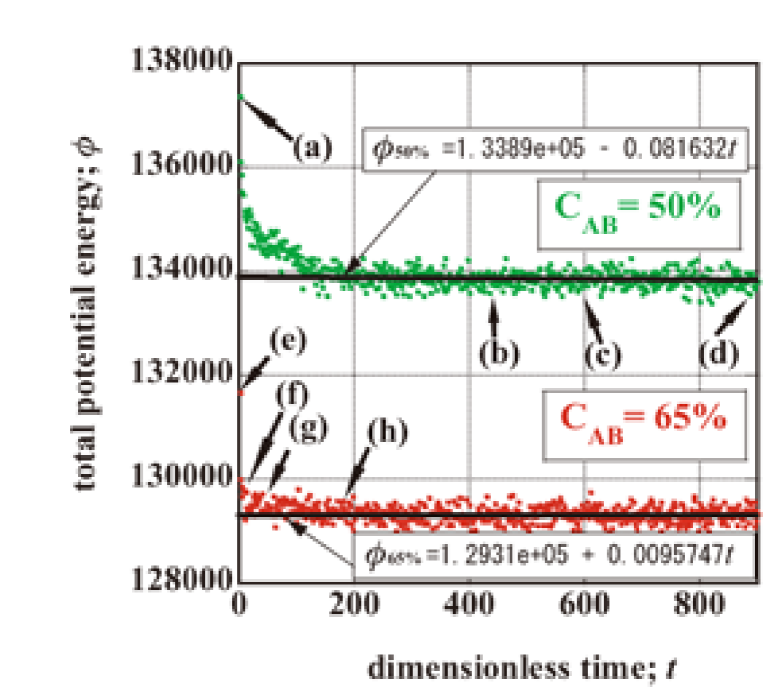
Figure 1: Time evolution of total potential energy. Green and red dots denote total potential energy for concentration of AB dimes $c_{\rm AB}=$ 50%, and 65 %, respectively. Dimensionless temperature is kept to $T=0.5.$ We make snapshots at eight times, i.e., $t=$0 (a), 450 (b), 600 (c), 900 (d) for $c_{\rm AB}=$ 50%, and $t=$0 (e), 30 (f), 75 (g), 195 (h) for $c_{\rm AB}=$ 65%. The snapshots are drawn in Figs. 2 and 3. Using the least squares method, we fit data in the region of $t\geq 200$ to liner functions.

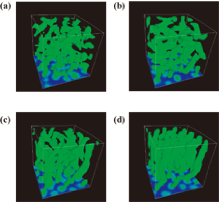
Figure 2: Snapshots of time evolution of self-assembly for $c_{\rm AB}=$ 50% at $T=0.5$. As the initial configuration(a), AB dimers and W monomers are distributed randomly in the simulation box. Velocities of all particles are distributed following Maxwell distribution. To make self-assembled structure of supramolecule clearly understandable, we pick up surface of the self-assembled structure, and interpolate the surface as if surface were continuous body. As time passes, hexagonal structure (${\rm H}_{1}$) grows like $t=$450 (b), 600 (c), 900 (d).

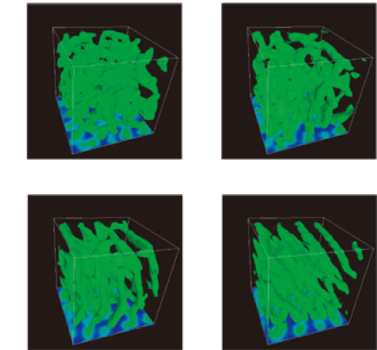
Figure 3: Snapshots of time evolution of self-assembly for $c_{\rm AB}=$ 65% at $T=0.5$. Visualization method, interaction forces, system size and other physical quantities except concentration of AB dimes are the same values as Fig. 1. As time passes, lamellar structure (${\rm L}_{\alpha}$) grows like $t=$0 (e), 30 (f), 75 (g), 195 (h). The time to form the self-assembled structure is shorter than ${\rm H}_{1}$ phase.

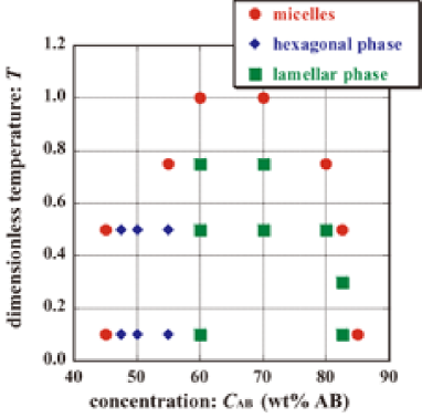
Figure 4: Phase diagram of AB dimers in solution W monomers. Horizontal axis is concentration of AB dimers $C_{\rm AB}$. Vertical one is dimensionless temperature $T$. Filled circles denote the micelles phase (${\rm L}_{\rm 1}$). Hexagonal (${\rm H}_{1}$) and lamellar (${\rm L}_{\alpha}$) phases are indicated by filled diamonds and squares, respectively. This phase diagram is qualitatively consistent with the previous work by Jury et al.[5].

RESULTS AND DISCUSSION

We found that it takes a longer time to form the hexagonal phase (${\rm H}_{1}$) than the lamellar phase $({\rm L}_{\alpha})$ where the system has higher order than ${\rm H}_{1}$ phase. This behavior is different from ordinary structure formation, where it takes a longer time to form the higher ordered phase than to form the lower ordered phase.

We would reach the conclusion that, in the process of structure formation in lamellar phase, the lamellar structure grows up directly from randomly distributed configuration of AB dimers. This behavior is contrary to our expected scenario that hexagonal cylinder structure grows first, then the hexagonal cylinders coalesce and finally lamellar appears.

Concerning the simulation model, it is easy to extend model of amphiphilic molecules for the chain-like configuration. We have already studied the dependence of interaction parameter of phase diagram[8].

References

- [1] P. J. Hoogerbrugge and J. M. V. A. Koelman. “simulating microscopic hydrocynamic phenomena with dissipative particle dynamics”. Europhys. Lett., 19:155, 1992.
- [2] R. D. Groot and P. B. Warren. “dissipative particle dynamics: Bridging the gap between atomistic and mesoscopic simulation”. J. Chem. Phys., 107:4423, 1997.
- [3] R. D. Groot and T. J. Madden. “dynamic simulation of diblock copolymer microphase separation”. J. Chem. Phys., 108:8713, 1998.
- [4] R. D. Groot and K. L. Rabone. “mesoscopic simulation of cell membrane damage, morphology change and rupture by nonionics surfactants”. Biophys. J., 81:725, 2001.
- [5] S. Jury, P. Bladon, M. Cates, S. Krishna, M. Hagen, N. Ruddock, and P. Warren. “simulation of amphiphilic mesophases using dissipative particle dynamics”. Phys. Chem. Chem. Phys., 1:2051, 1999.
- [6] D. J. Mitchell, G. J. T. Tiddy, and L. Waring. “phase behaviour of polyoxyethylene surfactants with water”. J. Chem. Soc., Faraday Trans. 1, 79:975, 1983.
- [7] P. Español and P. Warren. “statistical mechanics of dissipative particle dynamics”. Europhys. Lett., 30:191, 1995.
- [8] H. Nakamura. in preparation to submit.