Nematic textures in spherical shells.

Abstract

The equilibrium texture of nematic shells is studied as a function of their thickness. For ultrathin shells the ground state has four short $\frac{1}{2}$ disclination lines but, as the thickness of the film increases, a three dimensional escaped configuration composed of two pairs of half-hedgehogs becomes energetically favorable. We derive an exact solution for the nematic ground state in the one Frank constant approximation and study the stability of the corresponding texture against thermal fluctuations.

I Introduction

The study of liquid crystal phases benefits from geometrical reasoning in two important ways. Firstly, liquid crystal elasticity can often be cast in terms of the curvature of equipotential lines (or surfaces) that map out the corresponding textures. Second, the observed textures are strongly affected by geometric and topological constraints imposed by the presence of boundaries confining the system. The liquid crystal ground state results from the competition between the energetic requirement of minimizing the ”curvature of the texture” and the geometric frustration introduced by boundaries that impart a preferred curvature at the edge of the sample that often cannot propagate across the system deGennesbook ; Kleman-book ; MKleman .

The boundary conditions can be controlled experimentally with the possibility of designing molecular systems with intriguing technological applications Kami03 . For example, colloidal particles coated by a very thin nematic layer have in their ground state four disclinations sitting at the vertices of a tetrahedron. Each coated colloidal particle can then be viewed as the fundamental building block of a self assembled lattice with tetravalent coordination. The ”bonds” between the colloidal particles could be provided by chemical linkers attached at the four ”bald spots” at the cores of the four disclinations present in each colloid Nels02 . A second example, is provided by self-assembled systems of block copolymers sega03 which are a promising tool for ”soft lithography” on both flat and curved substrates Park-Chaikin97 . In addition, liquid crystals in confined geometries provide an arena for physicists and mathematicians interested in applications of geometrical and topological ideas to material science Kami02 ; Lavr98 ; Craw96 .

In this work we present a theoretical study of liquid crystal phases (focusing on vector, nematic and hexatic order) confined in a spherical shell of varying thickness with the director assumed to be tangent to the two interfaces. We first consider the two dimensional regime where a nematic film coats a quenched spherical surface such as a colloidal particle in solution or the interface of, say, a water droplet in oil. The presence of topological defects in the ground state for ordered states on spherical surfaces is unavoidable Nels83 ; Mack91 ; lube92 . Recent experimental and theoretical investigations of spherical crystallography have provided an alternative context to study the constraints posed by the compactness of the underlying curved space bowi2000 ; baus03 . More recent explorations have concentrated on 2D ordered phases confined to interfaces of varying Gaussian curvature Bowi03 ; ViteNels04 ; ViteTurn05 as well as dynamically fluctuating surfaces Park96 ; Lenz03 .

As the thickness of a nematic film increases, an escaped three dimensional texture, also strongly influenced by the spherical topology and the boundary conditions, become energetically favored with respect to planar textures. This instability destabilizes the tetravalent nematic texture on colloids. In this paper, we estimate the thickness of the nematic film above which a texture with four radial disclination lines of charge $s=\frac{1}{2}$ becomes unstable to four half-hedgehogs. The two competing textures studied in this paper are shown in Fig. 1. We also discuss the possibility of hysteresis between the two textures.

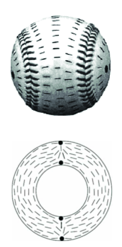
Figure 1: (Top panel) Two-dimensional texture characterized by four short disclination lines at the vertices of a tetrahedron inscribed in the sphere. The surface texture shown (inscribed on the surface of a baseball) is invariant throughout the thickness of the shell. (Bottom panel) Cut view of the escaped three dimensional texture given by two pairs of half hedgehogs located at the north and south poles of the sphere.

The organization of this paper is as follows. In section II we derive exact solutions for the ground state of spherical films of tilted molecules and nematogens within isotropic elasticity by using the method of conformal mappings. In the notation of References Nels02 ; lube92 , these situations correspond to order parameters described by a bond angle with $p=1,2$ fold symmetry in the tangent plane of the sphere (see Appendix A). A mathematical justification for our approach is provided in Appendix B, where the same technique is illustrated in the context of a more familiar flat space problem. In section III we study the stability of liquid crystal textures to thermal fluctuations by means of a normal mode analysis whose details are relegated to Appendices A and C. The stability of the valence-four texture against escaped solutions is considered in section IV where a phase diagram is derived with the thickness as a control parameter. The texture distortions caused by the elastic anisotropy between bend and splay deformations are briefly considered in section V.

II Textures

The liquid crystal free energy for molecules embedded in an arbitrary frozen surface can be written in the one constant approximation as

$$F=\frac{K}{2}\int dA\!\!\!\!\!\quad D_{i}n^{j}({\bf u})D^{i}n_{j}({\bf u})\!\!\!\!\quad,$$ (1)

where ${\bf u}=\{u_{1},u_{2}\}$ is a set of internal coordinates, ${\bf n}({\bf u})$ is the liquid crystal director defined in the tangent plane, $D_{i}$ is the covariant derivative with respect to the metric of the surface and $dA$ is the infinitesimal surface area Nels87 ; Davi87 ; Park96 ; Davidreview . The free energy of Eq.(1) is invariant upon rotating each molecule n$(u)$ by the same (arbitrary) angle with respect to any axis of rotation perpendicular to the local tangent plane. The treatment of systems with a p-fold symmetry is straightforward provided that the one Frank constant approximation is used for $p=1$ and $p=2$ and the consequences of any additional couplings to curvature neglected Davi87 . This choice of free energy implies that the minimal energy configuration will be given locally by neighboring ${\bf n}({\bf u})$ vectors which differ only by parallel transport. The curvature of the surface induces ”frustration” in the texture. In fact, by Gauss’ ”Theorema egregium” Kami02 , tangent vectors parallel transported along a closed loop are rotated by an amount equal to the Gaussian curvature integrated over the enclosed area. On a sphere, this theorem insures that the nematic ground state always has four excess disclinations Nels83 ; lube92 . More generally, the sum of the topological charges on any closed surface is equal to the integrated Gaussian curvature, implying a minimum of $2$ and $6$ disclinations in the ground state of tilted molecules and hexatics, respectively.

We introduce a local angle field $\alpha({\bf u})$, corresponding to the angle between ${\bf n}({\bf u})$ and an arbitrary local reference frame, we can rewrite the free energy introduced in Eq.(1) as:

$$F=\frac{1}{2}K\int dS\!\!\!\!\!\quad g^{ij}(\partial_{i}\alpha-A_{i})(\partial_{j}\alpha-A_{j})\!\!\!\!\quad,$$ (2)

where $dS=d^{2}u\sqrt{g}$, $g$ is the determinant of the metric tensor $g_{ij}$ and $A_{i}$ is the spin-connection whose curl is the Gaussian curvature $G({\bf u})$ Davidreview ; Kami02 . On a sphere of radius $R$ parametrized by polar coordinates $(\theta,\phi)$, the only non vanishing components of the (inverse) metric tensor are $g^{rr}=\frac{1}{R\sin\theta}$ and $g^{\phi\phi}=\frac{1}{R}$. A convenient choice of of the spin connection (which plays the role of the vector potential) is discussed in Appendix A. The simplified free energy in Eq.(2) is the starting point of our analysis.

II.1 Tilted molecules on a sphere

The orientational order of molecules tilted by a constant angle with respect to a spherical interface can be modelled by a vector field $\textbf{n}(\theta,\phi)$ defined in the local tangent plane on which the molecule has a fixed length projection Mack91 . To determine the ground state of the liquid crystal texture, we minimize the Frank free energy of Eq.(2). As discussed above, the topological charges must sum up to $4\pi$, the integrated Gaussian curvature of the sphere Davidreview ; Kami02 . For a vector field ($p=1$) the texture with only two defects of charges $+2\pi$ minimizes the Frank free energy and satisfies the topological constraint. Since the defects repel each other they preferentially sit at two antipodal points that we can designate as the north and south pole of the sphere. If the splay and bend coupling constants of the nematic are equal, then there is a large degeneracy in the ground state arising from the invariance of the vector free energy in Eq.(2) under global rotations $\alpha(\bf{u})$$\rightarrow$$\alpha(\bf{u})$+c, where $\textbf{u}\equiv{\theta,\phi}$. One representative texture is a ”sink” and a ”source” of $\textbf{n}(\textbf{u})$ at the two poles. In this splay rich texture $\textbf{n}(\textbf{u})$ is parallel to the lines of longitude on a sphere. In a bend rich texture, related to the previous by a $\frac{\pi}{2}$ rotation about the local normal to the surface, $\textbf{n}(\textbf{u})$ is everywhere parallel to the lines of latitude. Any other rotation of $\textbf{n}(\textbf{u})$ that makes an arbitrary constant angle with respect to this texture is an acceptable solution for the ground state of the molecules.

As we now show, this degeneracy is lifted when $K_{3}\neq K_{1}$. Indeed the effect of distinct splay and bend elastic constants $K_{1}$ and $K_{3}$ (the twist elastic constant $K_{2}$ is absent in two dimensions) is to select the bend-rich texture if $K_{1}>K_{3}$ or the splay-rich one if $K_{3}>K_{1}$. The intermediate configurations obtained by a global rotation of the director are now unstable. Assume for simplicity that $K_{3}>K_{1}$. In this case, it is convenient to recast the Frank free energy (see Appendix A) as follows:

$$F=\frac{1}{2}\int d^{2}\textbf{x}\!\!\!\!\quad\sqrt{g}\!\!\!\!\quad[K_{1}\left(D_{i}\!\!\!\!\!\quad n^{j}\left)\!\!\!\!\quad\right(D^{i}\!\!\!\!\!\quad n^{j}\right)$$

$$+(K_{3}-K_{1})(\textbf{D}\times\textbf{n})^{2}]\!\!\!\!\quad,$$ (3)

where the covariant derivatives is expressed in terms of the Christoffel connection, $\Gamma\!\!\!\!\!\quad^{j}_{i\!\!\!\!\!\!\!\quad t}$ ,

$$D_{i}\!\!\!\!\!\quad n^{j}=\partial_{i}\!\!\!\!\!\quad n^{j}+\Gamma\!\!\!\!\!\quad^{j}_{i\!\!\!\!\!\!\!\quad t}\!\!\!\!\quad n^{t}\!\!\!\!\!\quad,$$ (4)

and the covariant form of the curl squared is Davidreview ; Weinberg-GRbook ,

$$(\nabla\times\textbf{n})^{2}\equiv\left(D_{i}\!\!\!\!\!\quad n_{j}-D_{j}\!\!\!\!\!\quad n_{i}\left)\!\!\!\!\quad\right(D^{i}\!\!\!\!\!\quad n^{j}-D^{j}\!\!\!\!\!\quad n^{i}\right)\!\!\!\!\quad.$$ (5)

The first term in Eq.(3) resembles the Frank free energy in the one coupling constant approximation and is minimized by choosing the sink-source (or ”lines of longitude”) solution. The second term (which is positive definite) will vanish for this texture since the sink-source texture is bend free. All other textures have a higher energy.

A similar argument can be used to prove that the two vortex-configuration which follows the lines of latitude is the minimum of the free energy when $K_{1}>K_{3}$ by rewriting the Frank free energy as

$$F=\frac{1}{2}\int d^{2}\textbf{x}\!\!\!\!\quad\sqrt{g}\!\!\!\!\quad[K_{3}\left(D_{i}\!\!\!\!\!\quad n^{j}\left)\!\!\!\!\quad\right(D^{i}\!\!\!\!\!\quad n_{j}\right)$$

$$+\left(K_{1}-K_{3}\right)(\textbf{D}\cdot\textbf{n})^{2}]\!\!\!\!\quad,$$ (6)

where the covariant form of the divergence reads

$$\textbf{D}\cdot\textbf{n}\equiv\frac{1}{\sqrt{g}}\partial_{i}\left(\sqrt{g}\!\!\!\!\!\quad n^{i}\right)\!\!\!\!\quad.$$ (7)

The latitudinal texture minimizes the first term of Eq.(6) while the second vanishes because this texture is splay free. Any deviation from the splay-free latitudinal texture will only increase the energy.

The energy of both textures can be expressed as a function of the anisotropy parameter, $\epsilon$, and the mean of the elastic constants, $K$,

$$\epsilon \equiv \frac{K_{3}-K_{1}}{K_{3}+K_{1}}\!\!\!\!\quad,$$ (8)

$$K \equiv \frac{K_{3}+K_{1}}{2}\!\!\!\!\quad,$$ (9)

and the radius of the sphere, $R$, scaled by the short distance cutoff $a$. The resulting free energy for arbitrary $\epsilon$ reads (see Eq.(86))

$$F=2\pi K\left(1-|\epsilon\!\!\!\!\quad|\right)\left(\ln\left[\frac{R}{a}\right]-0.3\right)\!\!\!\!\quad.$$ (10)

The conclusions of this section are summarized in Fig. 2 which suggests that there is a discontinuous first order transition when $\epsilon$ passes through zero. This analysis mirrors similar arguments valid in the plane chandra-book .

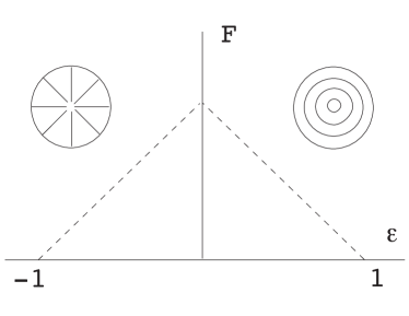
Figure 2: Schematic illustration of the phase diagram of the texture of tilted molecules on a sphere as a function of the anisotropy parameter $\epsilon$ superimposed on a plot of the free energy, $F$, stored in the texture versus $\epsilon$. The two competing ground states (top view) are characterized by either pure bend (lines of longitude configuration at left) or pure splay (lines of latitude configuration at right).

II.2 Nematic Texture

The nematic texture of very thin spherical shells of nematic liquid crystal with tangential boundary conditions can be analyzed within the one Frank constant approximation by using the method of conformal mappings whose mathematical justification is illustrated in Appendix B by means of a simpler example.

An elegant argument introduced by Lubensky and Prost in Ref.lube92 shows that the ground state of nematogens on a sphere is given by $4$ disclinations of topological charge $s=1/2$ sitting at the vertexes of a tetrahedron. The energy of single disclinations is proportional to the square of its strength. As a result, the longitudinal and latitudinal textures derived for tilted molecules in section II.1 are unstable since their energies can be lowered by splitting each $s=1$ defect at the north and south pole into two $s=1/2$ disclinations and letting them relax to their equilibrium positions at the vertexes of a tetrahedron where they are as far away from each other as possible. According to a calculation in Ref.lube92 , the energy $F_{s}$ of a sphere of radius $R$ with in plane orientational order and $2n$ interacting minimal disclinations for a p-fold order parameter is given by

$$F_{s}=2\pi K\!\!\!\!\quad h\left[\frac{1}{p}\ln\left(\frac{4p^{2}R}{a}\right)+c_{p}\right]\!\!\!\!\quad.$$ (11)

where the $\{c_{p}\}$ are constants depending on the symmetry of the order parameter and the defect core energy while $h$ is the thickness of the liquid crystal layer. The numerical values of the relevant constants are $c_{1}=0$ and $c_{2}\simeq-0.2$. When $p=2$ is chosen in Eq.(11) the elastic energy is indeed smaller than the corresponding value for $p=1$ in the limit $R\gg a$, in agreement with related arguments given in Ref.Nels02 .

To obtain an algebraic expression for the texture we proceed as illustrated in Appendix B and seek a function $\Omega(x,y,z)=\Phi(x,y,z)+i\Psi(x,y,z)$ which is harmonic on the sphere except for two arcs connecting the defects in pairs. The calculation for nematogens described below was suggested to us by F. Dyson Dyson . The function $\Phi(x,y,z)$, which we can interpret as an electrostatic potential, takes equal and opposite values on the two arcs and is equal to zero on a baseball-like seam (see Fig. 3) which divides the sphere into two congruent regions.

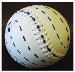
Figure 3: Schematic illustration of the baseball texture of a thin nematic shell. The same texture is reproduced from a different perspective in the top panel of Fig. 1.

The nematic director is then oriented (up to a global rotation) along the contour lines of $\Phi(x,y,z)$, that is the equipotential lines of this ”curved space capacitor”. In this analogy, the contour lines of $\Psi(x,y,z)$ are electric field lines, hence they correspond to a valid texture where the director is rotated locally by $\frac{\pi}{2}$ with respect to the equipotential lines. The arcs can be either great-circle arcs extending more than half way round the sphere or short great-circles arcs connecting the same pair of defects along the shortest path. The first choice leads to equipotential lines whose seam resembles in shape that of a baseball. If the second choice is made the pattern of equipotential lines would not deviate much from concentric circles and the seam would look more like the seam of a cricket ball. We will explicitly show that the two choices are equivalent since the equipotential lines of the first solution are field lines of the second and vice versa.

We choose the arcs connecting the defect pairs along great circles and we take the four defects labelled by A, B, C, D to lie at the vertices of a tetrahedron inscribed on a sphere of radius $1$ and whose north and south poles are $N=(0,0,1)$ and $S=(0,0,-1)$ respectively

$$A = \frac{1}{\sqrt{3}}(1,1,1)\!\!\!\quad,\!\!\quad B=\frac{1}{\sqrt{3}}(-1,-1,1)\!\!\!\quad,$$

$$C = \frac{1}{\sqrt{3}}(-1,1,-1)\!\!\!\quad,\!\!\quad D=\frac{1}{\sqrt{3}}(1,-1,-1)\!\!\!\quad.$$ (12)

We now perform a stereographic projection (see Fig. 4)

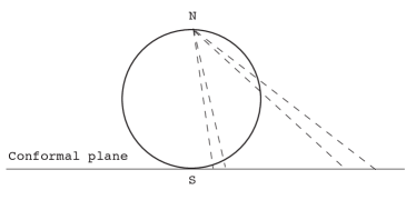
Figure 4: Graphical construction of the stereographic projection. Regions close to the north pole have larger images in the conformal plane than regions of equal areas close to the south pole. The stereographic projection preserves the topology of the surface provided all points at infinity are identified with the north pole.

that maps every point on a unit sphere centered on the origin onto the plane $z=-1$ according to the rule

$$\left(\begin{array}[]{c}x\\ y\\ z\\ \end{array}\right)\rightarrow\left(\begin{array}[]{c}a\\ b\\ -1\\ \end{array}\right)\!\!\!\quad.$$ (19)

The coordinates of the image points (connected to points on the sphere by dashed lines in Fig. 4) are given by

$$a = \frac{2x}{1-z}\!\!\!\quad,$$

$$b = \frac{2y}{1-z}\!\!\!\quad.$$ (20)

Upon transforming to a complex coordinate $w=a+ib$, the four tetrahedral points of Eq.(12) are mapped onto

$$A^{\prime} = p\!\!\!\!\quad(1+i)\!\!\!\quad,\!\!\quad B^{\prime}=p\!\!\!\!\quad(-1-i)\!\!\!\quad,$$

$$C^{\prime} = q\!\!\!\!\quad(-1+i)\!\!\!\!\quad,\!\!\quad D^{\prime}=q\!\!\!\!\quad(1-i)\!\!\!\quad,$$ (21)

where

$$p=\sqrt{3}+1\!\!\!\quad,\!\!\!\quad q=\sqrt{3}-1\!\!\!\quad.$$ (22)

(In this section $p$ does not refer to the symmetry of the order parameter). The great arc passing through the south pole (corresponding to one capacitor plate in the electrostatic analogy) maps onto the segment $A^{\prime}B^{\prime}$, as illustrated schematically in the top panel of Fig. 5, while the great arc through the north pole

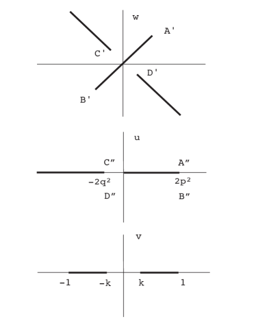
Figure 5: Illustration of the change in the branch cut structures of the complex function $\Omega(v)$ describing the nematic texture after performing a series of conformal transformations. In the top panel we have simply performed a stereographic projection from the sphere. The middle panel shows the ”fold up” transformation of Eq.(23) whereas the bottom panel corresponds to the transformation in Eq.(27) that symmetrizes the positions of the cuts.

maps onto the two semi-infinite segments of the line $a+b=0$ which bracket $C^{\prime}D^{\prime}$. We can fold the two cuts in the $w$ plane back on top of each other by mapping the $w$ plane onto the $u$ plane via

$$u=-iw^{2}\!\!\!\quad.$$ (23)

As shown in the middle panel of Fig. 5, the images à and B̃ of A’ and B’ now both lie on the real axis at $2p^{2}$ while the images of C’ and D’ now lie at $-2q^{2}$. The two cuts in the $u$ plane are both on the real axis, running from zero to $2p^{2}$ and from $-2q^{2}$ to minus infinity. On the sphere, these correspond to geodesics connecting defects which stretch more than halfway around the sphere. In order to make the cuts symmetric with respect to the imaginary axis (see the bottom panel of Fig. 5) we search for a conformal transformation that maps the following four points in the complex $u$-plane to four points on the real axis of a complex $v$-plane

$$u_{0}=0 \rightarrow v_{0}=k\!\!\!\quad,$$

$$u_{1}=-2q^{2} \rightarrow v_{1}=-k\!\!\!\quad,$$

$$u_{2}=-\infty \rightarrow v_{2}=-1\!\!\!\quad,$$

$$u_{3}=2p^{2} \rightarrow v_{3}=1\!\!\!\quad.$$ (24)

In order to fully determine the conformal transformation we need to determine the value of $k$. This can be done by using a standard relation in the theory of conformal transformations Smirnov3.2

$$\frac{u_{0}-u_{1}}{u_{0}-u_{2}}\!\!\!\quad\frac{u_{3}-u_{2}}{u_{3}-u_{1}}=\frac{v_{0}-v_{1}}{v_{0}-v_{2}}\!\!\!\quad\frac{v_{3}-v_{2}}{v_{3}-v_{1}}\!\!\!\quad.$$ (25)

Upon inserting the points of Eq.(24) into Eq.(25), we determine the value of $k$ (less than one)

$$k=\frac{2\sqrt{2}-p}{p+2\sqrt{2}}\!\!\!\quad.$$ (26)

Equation (24) contains four independent relations so we are still left with three conditions to determine the three independent coefficients $\{\alpha,\!\!\!\!\!\quad\beta,\!\!\!\!\!\quad\delta\}$ of the bilinear conformal transformation that implements the mapping illustrated pictorially in the bottom plate of Fig. 5

$$v=\frac{u+\delta}{\alpha\!\!\!\!\!\quad u+\beta}\!\!\!\quad.$$ (27)

The required coefficients needed to implement the mapping in Eq.(24) are

$$\alpha = -1\!\!\!\quad,$$

$$\beta = 2p\!\!\!\!\quad(2\sqrt{2}+p)\!\!\!\quad,$$

$$\delta = 2p\!\!\!\!\quad(2\sqrt{2}-p)\!\!\!\quad,$$ (28)

To solve Laplace’s equation, we desire a function $\Omega(v)$ which is analytic except on the two cuts on the real axis, and whose real part takes constant values on the cuts. By symmetry, $\Omega(v)$ is an odd function of v, and its real part $\Phi(v)$ is zero when the real part of v is zero. Therefore the image of the seam in the v plane is simply the imaginary axis $\Re e\!\!\!\!\quad v=0$. Upon substituting for $v$ using Equations (27) and (23), the condition $\Re e\!\!\!\!\quad v=0$ becomes

$$16+4p^{2}\Im m(w^{2})-|w|^{4}=0\!\!\!\quad,$$ (29)

With the help of Equations (20) and (19), we can now write down the equation of the seam explicitly in the original cartesian coordinates Dyson

$$z=(2+\sqrt{3})\!\!\!\!\!\quad xy\!\!\!\quad,$$ (30)

or in spherical polar coordinates $\{\phi,\!\!\!\!\!\!\quad\theta\}$ as

$$\frac{\cos\theta}{\sin^{2}\theta}=\left(1+\frac{\sqrt{3}}{2}\right)\sin 2\phi\!\!\!\quad.$$ (31)

The seam defined by the line of zero potential, is represented for different orientations of the sphere in Fig. 6.

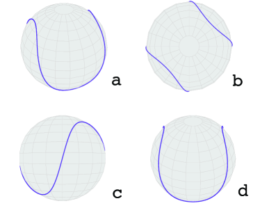
Figure 6: Different views of a track of parallel nematogens which partitions the sphere into two equal areas, each containing two $s=\frac{1}{2}$ disclination defects. It resembles a ”fattened” version of the seam of a baseball.

Its contour length $l$, on a unit radius ball, is readily calculated upon integrating the expression for the infinitesimal arc of the seam

$$dl=\sqrt{\sin^{2}\theta\left(\frac{d\phi}{d\theta}\right)^{2}+1}\!\!\quad d\theta\!\!\!\quad,$$ (32)

from $\theta_{min}\approx 0.69$ radians to $\theta_{max}\approx 2.44$ radians and multiplying the result by four in view of the symmetry of the seam. The values of $\theta_{min}$ and $\theta_{max}$ are obtained from Eq.(31) by setting $\phi$ equal to $\frac{\pi}{4}$ and $\frac{3\pi}{4}$ respectively. Upon using Eq.(31) to substitute $\phi(\theta)$ in Eq.(32), we obtain $l\simeq 9.09$ for a sphere of unit radius. The seam is longer than the equatorial circumference by slightly less than $50\%$.

The branch cut structure in the $v$ plane is sufficiently simple to allow a guess of the corresponding analytic function $\Omega(v)$. A function with cuts from $k$ to $1$ and $-k$ to $-1$, whose real part is equal and opposite on the two cuts and with a single imaginary period around any curve separating the cuts is easily identified to be a standard elliptic integral

$$\Omega(v)=\int_{0}^{v}\left[(k^{2}-t^{2})(1-t^{2})\right]^{-\frac{1}{2}}dt\!\!\!\quad.$$ (33)

with $v$ given in terms of $w$ by Equations (23) and (27). The nematic director is oriented (up to a global rotation) along the contour lines of the imaginary or (real part) of $\Omega(v)$. The equipotential (red) and field lines (black) of $\Omega(v)$ are conveniently plotted using the stereographic projection plane $w=a+ib$ in Fig. 7 along with the positions of the disclinations (green dots).

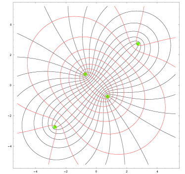
Figure 7: Illustration of the nematic texture in stereographic projection (Color online). The red and black field lines correspond to two energetically degenerate (in the one Frank constant approximation) families of bend and splay rich textures. The dots indicate the four tetrahedral $s=\frac{1}{2}$ disclination defects.

It is easy to switch from the stereographic-projection plane $w=a+ib$ of Fig. 7 to spherical polar coordinates $(\theta,\phi)$ by using the relation (reviewed in Appendix B),

$$w=2R\cot\left(\frac{\theta}{2}\right)e^{i\phi}\!\!\!\quad,$$ (34)

where $R$ is the radius of the sphere.

If we had constructed the base-ball with cuts along the $short$ geodesics connecting the defects, then the form of the texture given in Eq.(33) would be the same, but the parameter $k$ in the elliptic integral would be given by

$$k=(\sqrt{3}-\sqrt{2})^{2}(\sqrt{2}+1)^{2}\!\!\!\quad,$$ (35)

instead of Eq.(26). The equation for the seam becomes

$$z=-(2-\sqrt{3})\!\!\!\!\quad xy\!\!\!\quad$$ (36)

and the corresponding equipotential and field lines are plotted in black and red respectively in Fig. 7. The expression reads

$$\frac{\cos\theta}{\sin^{2}\theta}=-\left(1-\frac{\sqrt{3}}{2}\right)\sin 2\phi\!\!\!\quad,$$ (37)

in spherical polar coordinates, and leads to the same contour length $l$ as Eq.(31). Thus the two choices of arcs lead to two equivalent textures differing only by a $\frac{\pi}{2}$ about the local normal. As in Section II.1, the degeneracy in energy between the red and black flow lines in Fig. 7 is lifted upon considering the effect of elastic anisotropy generated by a different energy cost for bend and splay.

III Stability of liquid crystal textures to thermal fluctuations

In this section, we study the stability of liquid crystal ground states to thermal fluctuations Nels02 . To explore the fidelity of directional bonds at finite temperatures, we employ a Coulomb gas representation of the liquid crystal free energy (in the one Frank constant approximation) obtained by substituting in Eq.(2) the relation

$$\gamma^{\alpha\beta}\partial_{\alpha}(\partial_{\beta}\theta-A_{\beta})=s({\bf u})-G({\bf u})\equiv n({\bf u})\!\!\!\!\quad,$$ (38)

where $\gamma^{\alpha\beta}$ is the covariant antisymmetric tensor Davidreview , $G({\bf u})$ is the Gaussian curvature and $s({\bf u})\equiv\frac{1}{\sqrt{g}}\sum_{i=1}^{N_{d}}q_{i}\delta({\bf u}-{\bf u}_{i})$ is the disclination density with $N_{d}$ defects of charge $q_{i}$ at positions ${\bf u}_{i}$. The final result is an effective free energy whose basic degrees of freedom are the defects themselves Park96 ; bowi2000 ; Nels87 :

$$F = \frac{K}{2}\int\!dA\!\!\!\!\!\quad\int\!dA^{\prime}\!\!\!\quad n({\bf u})\!\!\!\quad\Gamma({\bf u},{\bf u}^{\prime})\!\!\!\quad n({\bf u}^{\prime})\!\!\!\!\quad.$$ (39)

The Green’s function $\Gamma({\bf u},{\bf u}^{\prime})$ is calculated (see Appendix A) by inverting the Laplacian defined on the sphere

$$\Gamma({\bf u},{\bf u}^{\prime})\equiv-\left(\frac{1}{\Delta}\right)_{{\bf u}{\bf u}^{\prime}}\!\!\!\!\quad,$$ (40)

and we have suppressed for now defect core energy contributions which reflect the physics at microscopic length scales. Equations (38) and (39) can be understood by analogy to two dimensional electrostatics, with the Gaussian curvature $G({\bf u})$ (with sign reversed) playing the role of a uniform background charge distribution and the topological defects appearing as point-like sources with electrostatic charges equal to their topological charge $q_{i}$. The charge $q$ can be defined by the amount $\theta$ increases along a counterclockwise path enclosing the defect’s core. On a generic surface, the defects tend to position themselves so that the Gaussian curvature is screened: typically, the positive ones are attracted to peaks and valleys while the negative ones to the saddles of the surface ViteNels04 ; ViteTurn05 . This geometric potential is ruled out by symmetry on an undeformed sphere since the Gaussian curvature is constant. The Gaussian curvature plays the role of a uniform background charge fixing the net charge of the defects consistent with the topological constraint imposed by the Poincare-Hopf theorem (see section II and References Kami02 ; Needham-book ). The equilibrium positions of the defects are then determined only by defect-defect interactions which are proportional to the logarithm of their chordal distance (see Appendix A) according to

$$F=-\frac{\pi K}{2p^{2}}\sum_{i\neq j}n_{i}n_{j}\ln\left[1-\cos\beta_{ij}\right]\!\!\!\!\quad,$$ (41)

where the integers $n_{i}$ and $n_{j}$ describing the singularities associated with each defect, and the integer $p$ controls the period $\frac{2\pi}{p}$ of the orientational order parameter. The ”topological charge” describing the rotation of the order parameter around each defect is given by $s_{j}=\frac{n}{p}$. The geodesic angle $\beta_{ij}$ subtended by the two defects at positions $\bf{u}_{i}=\{\theta_{i},\phi_{i}\}$ and $\bf{u}_{j}=\{\theta_{j},\phi_{j}\}$ can be conveniently recast in terms of their spherical polar coordinates

$$\cos\beta_{ij}=\cos\theta_{i}\cos\theta_{j}+\sin\theta_{i}\sin\theta_{j}\cos\left[\phi_{i}-\phi_{j}\right]\!\!\!\!\quad.$$ (42)

As a simple example, we first consider the case of a $Z=2$ colloidal particle (p=1) with two antipodal defects of index $1$. We can study the effect of thermal disruption of the ground state by setting $\beta_{ij}=\pi+\theta$ in Eq.(41) and expanding in the bending angle $\theta$. The resulting free energy, apart from an additive constant, reads

$$F\approx\frac{\pi K}{4}\!\!\!\!\quad\theta^{2}\!\!\!\!\quad.$$ (43)

Upon applying the equipartition theorem we obtain in the limit $K\gg k_{B}T$ Nels02

$$\langle\cos\beta_{ij}\rangle \approx -1+\frac{1}{2}\langle\theta^{2}\rangle\!\!\!\!\quad,$$ (44)

$$\approx -1+\frac{k_{B}T}{\pi K}\!\!\!\!\quad,$$

which describes the fidelity of $\pi$ antipodal ”bonds” of a divalent colloidal particle.

The effect of thermal fluctuations on the tetrahedral ground state of nematic molecules confined on the sphere (p=2 and all $s_{j}=\frac{1}{2}$) can be studied by means of a normal mode analysis. The basic results sketched in Nels02 were obtained by a slightly different method. Here we describe an alternative treatment in some detail and extend our analysis to hexatic and tetratic defect arrays (see Appendix C).

We start by defining a generalized array of defect coordinates $\{q_{i}\}$ as a $2N$ dimensional vector, where $N$ is the number of defects in the ground state (or, equivalently, the valence of the colloidal molecule). $N=4$ in the case of the tetrahedron. The first $N$ entries of the vector $\bf{q}$ are the longitudinal deviations of the $N$ defects from a perfect tetrahedral configuration while the remaining $N$ components describe defect displacements along the lines of latitude of a sphere of unit radius. As a result, the deviations of the $i^{th}$ defect from its equilibrium configuration $\{\theta_{i}\!\!\!\!\!\!\!\quad^{0},\phi_{i}\!\!\!\!\!\!\!\quad^{0}\}$ are parameterized by the two independent components of the vector $\bf{q}$

$$q_{i} = \delta\theta_{i}\!\!\!\!\quad,$$

$$q_{N+i} = \delta\phi_{i}\!\!\!\!\quad\sin(\theta_{i}\!\!\!\!\!\!\!\quad^{0})\!\!\!\!\quad.$$ (45)

The relations in Eq.(45) can be used to reexpress Eq.(42) in terms of the components of the displacements vector $q_{i}$, with the result,

$$\cos\beta_{ij}=\cos\left(\theta_{i}\!\!\!\!\!\!\!\quad^{0}+q_{i}\right)\cos\left(\theta_{j}\!\!\!\!\!\!\!\quad^{0}+q_{j}\right)+$$

$$\sin\left(\theta_{i}\!\!\!\!\!\!\!\quad^{0}+q_{i}\right)\sin\left(\theta_{j}\!\!\!\!\!\!\!\quad^{0}+q_{j}\right)\cos\left[\phi_{i}\!\!\!\!\!\!\!\quad^{0}-\phi_{j}\!\!\!\!\!\!\!\quad^{0}+\frac{q_{N+i}}{\sin\theta_{i}\!\!\!\!\!\!\!\quad^{0}}-\frac{q_{N+j}}{\sin\theta_{j}\!\!\!\!\!\!\!\quad^{0}}\right]\!\!\!\!\quad.$$ (46)

Upon substituting Eq.(46) in Eq.(41), the free energy $F$ can be expanded around the equilibrium configuration to quadratic order in $q_{i}$ with the result (apart from an additive constant)

$$F\approx\frac{1}{2}\sum_{ij}\!\!\!\!\quad M_{ij}\!\!\!\!\quad q_{i}\!\!\!\!\!\quad q_{j}\!\!\!\!\quad\!\!\!\!\quad,$$ (47)

where the matrix, $M_{ij}$, describing the deformation of the tetrahedral molecule is naturally defined as

$$M_{ij}=\left[\frac{\partial^{2}F}{\partial q_{i}\!\!\!\!\!\quad\partial q_{j}}\right]_{q_{i},q_{j}=0}\!\!\!\quad.$$ (48)

The eigenvalues of this matrix can be classified according to the irreducible representation of the symmetry group of the tetrahedron; their degeneracies can be determined purely from the group theoretical relation WilsonDeciusCross-book ; Landau-quantum-book

$$n^{(\gamma)}=\frac{1}{g}\sum_{i}\!\!\!\!\!\quad g_{i}\!\!\!\!\!\quad\chi_{i}^{(\gamma)\ast}\!\!\!\!\!\quad\chi_{i}^{(\Sigma)}\!\!\!\quad,$$ (49)

where $n^{(\gamma)}$ is the number of frequency degenerate normal modes that transform like the irreducible representation labeled by $\gamma$, $g_{i}$ is the number of symmetry operations of the tetrahedral point group in the i^th class, $g=\sum_{i}g_{i}=24$ is the total number of symmetry operation in the group, $\chi_{i}^{(\gamma)}$ is the character of the i^th class in the irreducible representation labelled by $\gamma$ while $\chi_{i}^{(\Sigma)}$ is the corresponding character for the reducible representation formed by the defects’ displacements.

The information necessary to apply Eq.(49) to a tetravalent colloid is collected in Table 1. The top row contains the five symmetry class $\{E,C_{3},C_{2},S_{4},\sigma_{d}\}$ contained in the tetrahedral point group $\Im_{d}$, corresponding respectively to the identity, three and two fold rotations, four fold rotatory-reflections and reflection through a plane of symmetry WilsonDeciusCross-book . The number of symmetry operations $g_{i}$ included in the i^th class also appears in the top row: thus, $\{g_{i}\}=\{1,8,3,6,6\}$ where the same ordering used above to list the classes has been adopted.

Table 1: Character for the irreducible representations of the tetrahedral point group together with the character of the eight-dimensional representation $\Sigma$ generated by the defect displacements of a tetravalent colloid.

$\Im_{d}$	$E$	8$C_{3}$	3$C_{2}$	6$S_{4}$	6$\sigma_{d}$
$A_{1}$	1	1	1	1	1
$A_{2}$	1	1	1	$-1$	$-1$
$E$	2	$-1$	2	0	0
$F_{1}$	3	0	$-1$	1	$-1$
$F_{2}$	3	0	$-1$	$-1$	1
$\Sigma$	8	$-1$	0	0	0

The left most column of Table 1 lists the one, two and three dimensional irreducible representations of the tetrahedral group $\{A_{1},A_{2},E,F_{1},F_{2}\}$, along with the eight dimensional representation $\Sigma$ generated by the defect displacements. The entries of the table list the characters corresponding to each class of the five irreducible representations, $\chi_{i}^{(\gamma)}$, and in the last row the corresponding characters, $\chi_{i}^{(\Sigma)}$, for the eight dimensional representation. The former are tabulated from standard group theoretical treatments while the latter needs to be worked out from the traces of the transformation matrices that describe how the displacement coordinates $q_{i}$ transform under the action of each symmetry element in the group. These manipulations are rather cumbersome, especially for the ”icosahedral molecule” arising when a spherical surface is coated with a pure hexatic layer (see Appendix C).

In the rich literature on molecular vibrations a set of empirical rules has been developed to write down the characters by examining only the transformation of the $three$ dimensional cartesian displacements of the few atoms whose equilibrium positions are not altered by the symmetry operation. In Appendix C we provide analogous rules that simplify the task of finding the $\chi_{i}^{(\Sigma)}$ characters by incorporating the constraint that each atom is confined on a sphere and hence only $two$ orthogonal displacements need to be considered as shown in Eq.(45).

The interested reader is referred to Appendix C for a more comprehensive mathematical justification of the normal mode analysis applied to the tetrahedral colloid and to the more complicated cases of hexatic $Z=12$ and tetratic order $Z=8$. Here, we simply summarize the results of applying Eq.(49) in conjunction with Table 1 to find the degeneracies of the eigenvalue spectrum of the matrix $M_{ij}$. The representation $\Sigma$ contains (only once) the three dimensional representations $F_{2}$ and $F_{1}$ as well as the two dimensional representation $E$.

$$\Sigma=F_{2}+F_{1}+E\!\!\!\quad.$$ (50)

The three normal coordinates with vanishing frequency correspond to the three rigid body rotations and belong to the $F_{1}$ irreducible representation WilsonDeciusCross-book ; Landau-quantum-book . We are left with a doublet ($E$) and a triplet ($F_{2}$) corresponding respectively to two shear-like twisting deformations of the tetrahedron and to three stretching and bending modes of the cords joining neighboring defects.

This symmetry analysis is confirmed by direct diagonalization of the matrix $M_{ij}$ which leads the following set of eigenvalues $\lambda_{i}$

$$\{\lambda_{i}\}=\frac{3\!\!\!\!\!\quad\pi\!\!\!\!\!\quad K}{8}\!\!\!\quad\{0,0,0,1,1,2,2,2\}\!\!\!\quad.$$ (51)

In Section C, we also list the eigenvectors $w_{i}$ of $M_{ij}$. The displacement coordinates are readily expressed in terms of the eigenvectors

$$q_{i}=U^{-1}_{ij}\!\!\!\!\!\quad w_{j}\!\!\!\quad,$$ (52)

where the unitary matrix $U$ diagonalizes $M$ and hence the free energy of Eq.(47) and is defined by

$$U\!\!\!\!\!\quad M\!\!\!\!\!\quad U^{-1}=Diag\!\!\!\!\!\quad(\lambda_{i})\!\!\!\quad.$$ (53)

Its construction is easily achieved by the standard Gram-Schmidt orthogonalization procedure to the eigenvectors $\{w_{i}\}=\{w_{1},...,w_{8}\}$, where the same ordering chosen in listing the eigenvalues in Eq.(51) is implicitly assumed. The resulting orthogonal basis vectors are the rows of the $8\times 8$ matrix $U$.

We are now in a position to evaluate $\langle\cos\beta_{ij}\rangle$ where the thermal average is performed with the Boltzman weight obtained from the free energy in Eq.(47) which is now diagonal. Note that for the tetrahedron any choice of pair of defects labelled by $i$ and $j$ (where $i\neq j$) will lead to the same answer, unlike the less symmetric cases of the twisted cube (p=4) and the icosahedron (p=6) considered in Appendix C. The bending angle $\cos\beta_{ij}$ in Eq.(46) can be Taylor expanded in the $q_{i}$. The resulting expression is rather cumbersome, but once the displacements $\{q_{i}\}$ are reexpressed in terms of the normal coordinates $\{w_{i}\}$ (by means of Eq.(52)), $\cos\beta_{ij}$ reduces to

$$\cos\beta_{ij}=-\frac{1}{3}+\frac{2}{9}\left(w_{6}^{2}+w_{7}^{2}+w_{8}^{2}\right)\!\!\!\quad,$$ (54)

where the only eigenmodes $\{w_{6},w_{7},w_{8}\}$ appearing in Eq.(54) correspond to the bending triplet of Eq.(51).

It is now easy to perform the thermal average by Gaussian integration of the energetically degenerate eigenmodes, with the result Nels02

$$\langle\cos\beta_{ij}\rangle = -\frac{1}{3}+\frac{2}{9}\!\!\!\!\!\quad\left(\langle w_{6}^{2}\rangle+\langle w_{7}^{2}\rangle+\langle w_{8}^{2}\rangle\right)$$ (55)

$$= -\frac{1}{3}+\frac{16\!\!\!\!\!\quad k_{B}\!\!\!\!\!\!\quad T}{9\pi K}\!\!\!\quad.$$

IV Valence transitions in thick nematic shells

In this section, we study the crossover from a two to three dimensional regime as the thickness of the spherical shell, $h$, increases. For thicker shells, three dimensional defect configurations (”escaped” in the third dimension) compete with the planar textures described in the previous sections, leading to a structural transition and a change in valence from $Z=4$ to $Z=2$ beyond a critical value of $h$.

We first consider the case of a cylindrical slab (or disk) of radius $R$ and thickness $h$ filled with a nematic whose director is tangent to the two circular faces Chic02 (see Fig. 8). This simpler geometry captures the essential features of the problem and provides a suitable starting point for understanding thin spherical shells (see Fig. 9).

IV.1 Slab geometry

To estimate the energy stored in the texture of Fig. 8, we coarse grain the system to ”blobs” of size $h$. The elastic energy arises from two sources: a long distance contribution from a radial texture associated with an $s=1$ disclination and a local energy cost for the elastic deformations inside the spherical blob in Fig. 8.

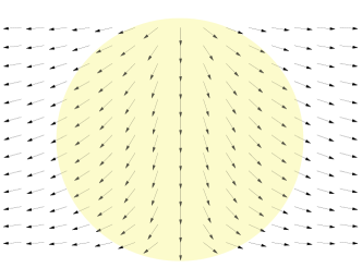
Figure 8: Side view of the 2D nematic texture ansatz solution in Eq.(60). The cylindrical slab has height $h$ and radius $R$. The arrows can be interpreted as flow lines of a fluid entering a narrow and long channel from a point source located on the top plate. To obtain the nematic texture the vectors need to be normalized and viewed as rods with both ends identified as shown in Fig. 9.

In the one Frank constant approximation, the former can be estimated as the energy $\pi Kh\ln\left(\frac{R}{h}\right)$ of a disclination whose enlarged ”core” of size $h$ is given by the spherical blob while the latter is roughly $4\pi Kh$, the energy of two half hedgehogs living inside the blob Stark01 .

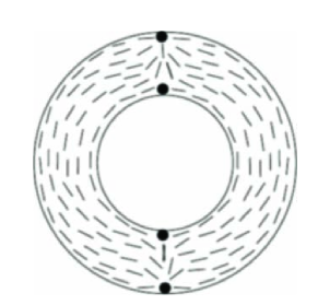
Figure 9: Nematic texture in a thin spherical shell. The nematic director near the pair of half hedgehogs indicated in the figure is well described by the one calculated for the slab in Fig. 8.

In view of the azimuthal symmetry of our configuration, the director, $\textbf{n}(\textbf{r},z)$, can be parameterized by the angle $\Theta(\textbf{r},z)$ formed with respect to the $\widehat{z}$ axis of the circular slab along the centers of the two half hedgehogs shown in Fig. 8

$$\textbf{n}(\textbf{r},z)=\sin\Theta(\textbf{r},z)\textbf{e}_{r}+\cos\Theta(\textbf{r},z)\textbf{e}_{z}\!\!\!\!\quad.$$ (56)

The energy density $f(\Theta)=\frac{1}{2}K_{1}\left(\nabla\cdot\textbf{n}\right)^{2}+\frac{1}{2}K_{3}\left(\nabla\times\textbf{n}\right)^{2}$ expressed in terms of the bond angle reads

$$f(\Theta) = \frac{K_{1}}{2}\left(\frac{\sin\Theta}{r}+\Theta_{r}\cos\Theta-\Theta_{z}\sin\Theta\right)^{2}$$ (57)

$$+ \frac{K_{3}}{2}\left(\Theta_{z}\cos\Theta+\Theta_{r}\sin\Theta\right)^{2}\!\!\!\!\quad.$$

where $K_{1}$ and $K_{3}$ are the splay and bend constants and $\Theta_{r}\equiv\frac{\partial\Theta}{\partial r}$ and $\Theta_{z}\equiv\frac{\partial\Theta}{\partial z}$ . In the one Frank constant approximation, minimization of the free energy leads to a non linear partial differential equation for the bond angle $\Theta(\textbf{r},z)$

$$\frac{1}{r}\frac{\partial}{\partial r}\left(r\frac{\partial\Theta}{\partial r}\right)+\frac{\partial^{2}\Theta}{\partial z^{2}}=\frac{\sin 2\Theta}{r^{2}}\!\!\!\!\quad.$$ (58)

The operator on the left arise from the Laplacian in cylindrical coordinates. Note there is no need to explicitly consider the azimuthal angle $\phi$ as an additional independent variable in view of the symmetry of the problem.

Instead of solving this partial differential equation, we follow a route analogous to that in Ref.Lube98 , that is we construct an $exact$ 2D solution for the liquid crystal problem and then rotate it along the axis $\widehat{z}$ to retrieve an $ansatz$ for the 3D director configuration. The 2D solution is the true minimum of the two dimensional liquid crystal elastic free energy while the 3D Ansatz does $\bf{not}$ minimize $f(\Theta)$ nor satisfy Eq.(58).

To solve the 2D problem we adopt the method of conformal mappings that simplifies the study of many complicated boundary problems in fluid dynamics and electrostatics Smirnov3.2 . Think of Fig. 8 as a source of fluid confined to flow in a narrow and long channel ($R\gg h$). The spherical ”half-hedgehog” corresponds to the source and the hyperbolic one at the top to the stagnation point of the flow. The complex potential $\Omega(w)$ of the desired flow is

$$\Omega(w)=Log\left(\sin\left(\frac{\pi w}{h}\right)-1\right)\!\!\!\!\quad,$$ (59)

where the complex variable is denoted by $w=r+iz$ to distinguish it from the $z$ coordinate along the axis of the cylinder. The velocity field is given by $\overline{\Omega^{\prime}(w)}$ and the corresponding complex nematic director $\textbf{n}(w)=\cos{\Theta}+i\sin{\Theta}$ is obtained by normalizing this vector field. Note that the prime in $\Omega^{\prime}(w)$ denotes the derivative with respect to $w$ of the complex function $\Omega=\Phi+i\Psi$ and we define $\overline{\Omega}\equiv\Phi-i\Psi$. A straightforward but tedious calculation (see Appendix B) leads the functional form of $\Theta(r,z)$ for a source at $z=-\frac{h}{2}$ and a stagnation point at $z=+\frac{h}{2}$, namely

$$\tan\Theta(r,z)=\sec\left(\frac{\pi z}{h}\right)\sinh\left(\frac{\pi r}{h}\right)\!\!\!\!\quad.$$ (60)

This trial solution respects the boundary conditions of the problem, has the correct short and long distance behavior in $r$ and the expected functional form near the source.

Upon inserting $\Theta(r,z)$ in Eq.(57) and integrating the energy density $f(\Theta)$ over the cylindrical volume of the slab, we obtain the total elastic energy $E_{1}$ stored in the field. The resulting energy $E_{1}$ does $\bf{not}$ rely on the assumption $R\gg h$, as can be explicitly checked numerically.

$$E_{1}=\pi Kh\left[\ln\left(\frac{R}{h}\right)+c\right]\!\!\!\!\quad,$$ (61)

where $c\approx 4.2$. Note that the functional dependence of $E_{1}$ on $R$ and $h$ matches the expectations from the blob argument. Indeed the prefactor of the logarithm is universal in the sense that it does not depend on the details of the trial solution near the hedgehogs, but only on its long distance behavior. By contrast, we expect the result quoted above for the coefficient $c$ to be only an estimate (an upper bound) since it relies on a $trial$ solution for $\Theta(r,z)$ that is not the absolute minimum of the free energy. Numerical studies carried out in Ref.Chic02 for the slab geometry reported that $c\approx 4.19$.

A competing energy minimum for the nematic is given by a planar texture with two $s=\frac{1}{2}$ disclination lines. Note that $+\frac{1}{2}$ lines cannot escape in the third dimension chandra-book . A tedious but straightforward calculation shows that the energy $E_{p}$ of the pair of disclination lines is given by

$$E_{p}=\frac{\pi}{2}Kh\left(\ln\left(\frac{R}{a}\right)-0.06+\frac{4\!\!\!\!\quad E_{c}}{\pi Kh}\right)\!\!\!\!\quad.$$ (62)

where $a$ is a macroscopic cutoff typically of the order of the molecular length. These two disclination repel each other, and are repelled by the circular boundary, leading to a separation of order $R$. The second term of Eq.(62), corresponding to the interaction of the two disclinations with the boundary and among themselves, is negligibly small. The third term accounts for the core energies of the two disclination lines $2E_{c}$. The combination $Kh$ is equal to the two dimensional coupling constant $K_{2D}$. The relevant dimensionless ratio is $\frac{E_{c}}{K_{2D}}$.

By setting $E_{p}=E_{1}$ we obtain the critical thickness $h^{*}$ above which the escaped ”half-hedgehogs” become energetically favored compared to a single $s=\frac{1}{2}$ disclination line:

$$h^{*}=e^{c^{\prime}}\sqrt{R\!\!\!\!\!\quad a}\!\!\quad.$$ (63)

The core energy terms in Eq.(62) reduce the previous estimate of $c$ to $c^{\prime}=c-\frac{2E_{c}}{\pi Kh}$. A similar analysis applies to spherical shells which we now discuss.

IV.2 Extrapolation to thin spherical shells

In principle, one could proceed along the same route as in the previous section and find a conformal mapping that provides a trial function for the bond angle $\Theta(\theta,r)$ corresponding to the texture shown in Fig. 9. This is possible but rather cumbersome. In the case of very thin shells one can adapt the slab calculation by noting again that the energy is composed of two parts. There is a long distance piece arising from ”combing the hair” of the nematic texture in the tangent plane of the sphere that we can read off from a suitable 2D calculation (see Appendix A) and the short distance contribution arising from the short distance contribution arising from the two pairs of half-hedgehogs at the north and south pole.

The energy $E_{d}$ of two short $+1$ disclination lines placed at antipodal points on a sphere (the north and south pole, say) can be estimated by performing a 2D calculation on the curved surface and simply multiplying the result by the thickness of the layer $h$

$$E_{d}=2\pi Kh\left(\ln\left(\frac{R}{a}\right)-0.3+\frac{E_{c}}{\pi Kh}\right)\!\!\!\!\quad,$$ (64)

where the middle term accounts for the interaction between the two disclinations in their equilibrium positions. Note that this result is accurate only up to factors of the order of $\left(\frac{h}{R}\right)$ since the explicit integration over the volume of the thin shell was bypassed. To obtain the energy of the escaped solution, the core size $a$ in Eq.(64) is rescaled to $h$. This will account for the integration of the energy density at distances of the order of a few $h\ll R$ from the two hedgehogs. In these portions of the shell the integrand reduces to the energy density of the two disclination problem and hence the integration can be easily carried out leading the result in Eq.(64) with a lower cutoff of the order $h$.

The energy stored in the remaining portions of the thin shell is approximately given by twice the energy $4.2\!\!\!\!\!\quad\pi Kh$ of the yellow blob of Fig. 8. This estimate neglects curvature corrections of the order of $\left(\frac{h}{R}\right)$ and arises because at distances of the order $h$ the spherical shell looks $locally$ like a flat circular slab as long as $h\ll R$. The resulting energy $E_{2}$ of the escaped configuration reads

$$E_{2}=2\pi Kh\left(\ln\left(\frac{R}{h}\right)-0.3+4.2\right)\!\!\!\!\quad.$$ (65)

Although the prefactor of the sub-leading term linear in $h$ has only been estimated, we expect that the coefficients of the logarithm, which arises from large scales compared to $h$, is exact. For a spherical shell whose radius $R$ is a hundred times its thickness, the corrections from higher powers of $\frac{h}{R}$ are indeed negligible. However for reasonable values of $\frac{R}{h}$, the logarithmic term of Eq.(65) is still comparable in magnitude to the ”sub-leading” one linear in $h$.

The energy $E_{4}$ of the tetravalent configuration can be evaluated using similar considerations, with the result

$$E_{4}=\pi Kh\left(\ln\left(\frac{R}{a}\right)-0.4+\frac{4E_{c}}{K\pi h}\right)\!\!\!\!\quad.$$ (66)

Upon setting $E_{4}=E_{2}$ we obtain the critical thickness $h^{*}$ below which the tetravalent configuration becomes energetically favored

$$h^{*}=e^{(4.1-\frac{2E_{c}}{K\pi h})}\sqrt{R\!\!\!\!\!\quad a}\!\!\quad.$$ (67)

The exponential prefactor arises from the terms linear in $h$ in Eq.(65), which cannot be ignored in estimating $h^{*}$ even in the limit $R\gg h$. Note that an accurate determination of the argument in the exponent would require knowledge of the core energies of the disclination lines. In fact, the exponential prefactor can be interpreted as a numerically significant rescaling of the core radius.

The energy barrier between these two coexisting minima of the free energy $f(\Theta)$ can be estimated by splitting the path connecting them in $\Theta$ space in two steps. First, consider a continuous deformation of the escaped texture of Fig. 9 obtained by appropriately rotating each nematigen until the $non-escaped$ solution (with two disclinations $lines$ of index one at the north and south pole) is recovered. This part of the path must be uphill in energy if the escaped solution was allowed to escape in the first place. The corresponding energy barrier $\Delta E$ is given approximately by the difference between $E_{d}$ as calculated in Eq.(64) and $E_{2}$ in Eq.(65)

$$\Delta E=2\pi Kh\left(\ln\left(\frac{h}{a}\right)-4.2\right)\!\!\!\!\quad.$$ (68)

The second step consists in letting each of the unstable disclination lines split in two $+\frac{1}{2}$ defects and subsequently separate them until they sit at the vertexes of a tetrahedron inscribed in the sphere. This portion of the path is downhill because the ”non-escaped” texture of valence $2$ is unstable. This can be proved by writing down the energy of the pair and show that it decreases monotonically as one separates them because of the ”electrostatic-like” repulsion lube92 ; ViteNels04 . As a result the energy barrier is simply the energy difference calculated in Eq.(68).

Upon inserting $K\approx 10^{-6}$ dyn in Eq.(68) and taking $k_{B}T\approx 4\!\!\!\!\quad 10^{-14}$ erg, as in Ref.Poul97 ; Stark01 , we obtain

$$\frac{\Delta E}{k_{B}T}\approx\frac{15h}{nm}\left(\ln\left(\frac{h}{a}\right)-4.2+\frac{E_{c}}{K\pi h}\right)\!\!\!\!\quad.$$ (69)

For shells with critical thickness $h^{*}$ Eq.(69) reduces to

$$\frac{\Delta E}{k_{B}T}\approx 10^{3}\sqrt{\frac{R}{a}}\!\!\!\!\quad\ln\left(\frac{R}{a}\right)\!\!\!\!\quad,$$ (70)

where a core size of the order of $10$ nm was assumed and the core energies were set to zero lube92 . This estimate indicates that the energy barrier is very high around $h^{*}$ suggesting that exchange between the two minima is unlikely to happen by thermal activation. In a monodisperse solution of shells with thickness $h$, the ratio between shells of the two valence will be given by their Boltzman factors as long as equilibrium is reached. If one engineers shells with thickness below $h^{*}$, the Z=4 configuration would be more likely.

V Conclusion

We have studied the crossover from the two dimensional regime of liquid crystals confined on a spherical surface to the full three dimensional problem in a spherical shell. For very thin shells, the nematic ground state has four disclination lines sitting at the vertices of a tetrahedron inscribed in the ball and whose texture approximately track the seam of a baseball. As the thickness increases, a competing three dimensional defected texture characterized by two pairs of half hedgehogs at the north and south pole becomes energetically favorable. For ultra-thin shells this instability is suppressed and one expects a defected ground state with tetravalent symmetry. Estimates of the stability of this texture to thermal fluctuations indicate that the vibrations around the equilibrium configurations of the defects should not be significant. The present analysis has been carried out primarily in the limit in which the elastic anisotropy parameter, $\epsilon=\frac{K_{3}-K_{1}}{K_{3}+K_{1}}\ll 1$.

We hope to extend our investigation with a systematic study of the effect of elastic anisotropy on the nematic texture. It is interesting to note that in the case of pure bend or splay (ie. $\epsilon=\pm 1$) the ground state is given by only two disclinations of unit index at the north and south pole. This suggests the possibility that the effect of the elastic anisotropy may not be limited to locally adjusting the orientation of the director but may induce a change in the inter-defect interaction and hence a distortion of the tetravalent equilibrium configuration. The limit of strong elastic anisotropy is also relevant to studies of the nematic to smectic transition in a spherical geometry for which the ratio of the bend to splay coupling constants $\frac{K_{3}}{K_{1}}$ is expected to diverge.

Additional experimental complications include the possibility of having a nematic layer of non constant thickness that would induce trapping of the defects in the regions where the layer is thinner. This effect may also induce a local transition to an escaped texture where the layer thickens in just one hemisphere so that two disclination lines of index $\frac{1}{2}$ are traded for a pair of half hedgehogs. If that happens shells with three-fold symmetry could be observed.

Appendix A Free energy of a vector field on a sphere

We start our analysis with the Frank free energy with splay and bend terms proportional to $K_{1}$ and $K_{3}$ and expressed in terms of the covariant derivative $D_{i}\!\!\!\!\!\quad n^{j}$

$$F = \frac{1}{2}\int d^{2}\textbf{x}\!\!\!\!\quad\sqrt{g}\!\!\!\!\quad[K_{1}\left(D_{i}\!\!\!\!\!\quad n^{i}\right)^{2}\!$$ (71)

$$+ K_{3}\left(D_{i}\!\!\!\!\!\quad n_{j}-D_{j}\!\!\!\!\!\quad n_{i}\right)\left(D^{i}\!\!\!\!\!\quad n^{j}-D^{j}\!\!\!\!\!\quad n^{i}\right)]\!\!\!\!\quad,$$

where

$$D_{i}\!\!\!\!\!\quad n^{j}=\partial_{i}\!\!\!\!\!\quad n^{j}+\Gamma\!\!\!\!\!\quad^{j}_{i\!\!\!\!\!\!\!\quad k}\!\!\!\!\quad n^{k}\!\!\!\!\!\quad.$$ (72)

The Christoffel connection $\Gamma\!\!\!\!\!\quad^{j}_{i\!\!\!\!\!\!\!\quad k}$ Weinberg-GRbook is unchanged if the lower indices $i$ and $k$ are interchanged. As a result, the covariant derivative $D_{i}$ can be replaced by $\partial_{i}$ in the second term of Eq.(71) because the covariant curl is antisymmetric. It follows that

$$\vec{D}\times\vec{n}=\nabla\times\vec{n}\!\!\!\!\!\quad.$$ (73)

The covariant form of the divergence is given by Weinberg-GRbook

$$D_{i}\!\!\!\!\!\quad n^{i}\equiv\frac{1}{\sqrt{g}}\!\!\!\!\quad\partial_{i}\left(\sqrt{g}\!\!\!\!\!\quad n^{i}\right)\!\!\!\!\quad.$$ (74)

For a rigid sphere of radius $R$ with polar coordinates $\{\theta,\phi\}$, we have $\sqrt{g}=R^{2}\sin\theta$, $\Gamma\!\!\!\!\!\quad^{\theta}_{\phi\!\!\!\!\!\!\!\quad\phi}=-\sin\theta\cos\theta$, $\Gamma\!\!\!\!\!\quad^{\phi}_{\phi\!\!\!\!\!\!\!\quad\theta}=\Gamma\!\!\!\!\!\quad^{\phi}_{\theta\!\!\!\!\!\!\!\quad\phi}=-\cot\theta$, and all other $\Gamma\!\!\!\!\!\quad^{j}_{i\!\!\!\!\!\!\!\quad k}=0$.

Upon adding and subtracting the expression for the curl of $\bf{n}$ multiplied by $K_{1}$ from the first and second term in Eq.(71) we obtain

$$F=\frac{1}{2}\int d^{2}\textbf{x}\!\!\!\!\quad\sqrt{g}\!\!\!\!\quad[K_{1}\left(D_{i}\!\!\!\!\!\quad n^{j}\left)\!\!\!\!\quad\right(D^{i}\!\!\!\!\!\quad n_{j}\right)$$

$$+(K_{3}-K_{1})(\nabla\times\textbf{n})^{2}]\!\!\!\!\quad.$$ (75)

Similarly, upon adding and subtracting the covariant divergence of $\bf{n}$ multiplied by $K_{3}$ from the second and first term in Eq.(71) we obtain

$$F=\frac{1}{2}\int d^{2}\textbf{x}\!\!\!\!\quad\sqrt{g}\!\!\!\!\quad[K_{3}\left(D_{i}\!\!\!\!\!\quad n^{j}\left)\!\!\!\!\quad\right(D^{i}\!\!\!\!\!\quad n_{j}\right)$$

$$+\left(K_{1}-K_{3}\right)(\nabla\cdot\textbf{n})^{2}]\!\!\!\!\quad.$$ (76)

Upon adding the two equivalent expressions for $F$ in Equations (75) and (76) and dividing by two we can express the free energy in terms of the constants

$$\epsilon \equiv \frac{K_{3}-K_{1}}{K_{3}+K_{1}}\!\!\!\!\quad,$$ (77)

$$K \equiv \frac{K_{3}+K_{1}}{2}\!\!\!\!\quad,$$ (78)

namely

$$F=\frac{K}{2}\int d^{2}\textbf{x}\!\!\!\!\quad\sqrt{g}\!\!\!\!\quad[\left(D_{i}\!\!\!\!\!\quad n^{j}\left)\!\!\!\!\quad\right(D^{i}\!\!\!\!\!\quad n_{j}\right)$$

$$+\epsilon\left((\nabla\times\textbf{n})^{2}-(\nabla\cdot\textbf{n})^{2}\right)]\!\!\!\!\quad.$$ (79)

We now parameterize the orientation of the unit vector $\bf{n}$ in terms of the bond angle field $\alpha(\theta,\phi)$ that it forms with respect to the longitudinal direction $\vec{e}$_θ which in polar coordinates $(\theta,\phi)$ is given by

$$\textbf{e}_{\theta}=R(\cos{\theta}\sin{\phi},\cos{\theta}\cos{\phi},-\sin{\theta})\!\!\!\!\quad,$$ (80)

while the orthogonal unit vector $\textbf{e}_{\phi}$ is given by

$$\textbf{e}_{\phi}=R(-\sin{\theta}\sin{\phi},\sin{\theta}\cos{\phi},0)\!\!\!\!\quad.$$ (81)

The components of the vector $\bf{n}$ with respect to $\vec{e}_{\phi}$ and $\vec{e}$_θ are given by

$$n^{\theta} = \frac{\cos\alpha}{R}\!\!\!\!\quad,$$ (82)

$$n^{\phi} = \frac{\sin\alpha}{R\sin\theta}\!\!\!\!\quad.$$ (83)

Upon substituting the relevant expressions for the non vanishing components of the connection in the covariant derivative (see Eq.(72)) and using Eq.(83), the free energy density $f(\theta,\phi)$ is given by

$$\frac{4R^{2}}{K_{1}+K_{3}}\!\!\!\!\quad f = \left(\frac{\partial\alpha}{\partial\theta}\right)^{2}+\Upsilon_{\alpha}\!\!\!\!\!\!\!\quad^{2}(\theta,\phi)$$ (84)

$$+ \epsilon\cos 2\alpha\left[\left(\frac{\partial\alpha}{\partial\theta}\right)^{2}-\Upsilon_{\alpha}\!\!\!\!\!\!\!\quad^{2}(\theta,\phi)\right]$$

$$+ 2\epsilon\sin 2\alpha\left(\frac{\partial\alpha}{\partial\theta}\right)\Upsilon_{\alpha}(\theta,\phi)\!\!\!\!\quad,$$

where the $\alpha$-dependent function $\Upsilon_{\alpha}(\theta,\phi)$ is

$$\Upsilon_{\alpha}(\theta,\phi)\equiv\frac{1}{\sin\theta}\left(\frac{\partial\alpha}{\partial\phi}+\cos\theta\right)\!\!\!\!\quad.$$ (85)

The energies of the latitudinal ($\alpha=\pi/2$) and longitudinal ($\alpha=0$) tilted-molecules textures favored for $\epsilon$ less or greater than zero respectively (see section II.1) are easily determined by substituting the appropriate $\alpha$ and $\epsilon$ in Eq.(84). After integrating the free energy density $f$ in Eq.(84) we obtain

$$F = 2\pi K(1-|\epsilon|)\int_{\frac{a}{R}}^{\frac{\pi}{2}}\frac{\cos^{2}(\theta)}{\sin(\theta)}\!\!\!\!\!\quad d\theta$$ (86)

$$= 2\pi K(1-|\epsilon|)\left(\ln\left(\frac{2R}{a}\right)-1\right)+2E_{c}\!\!\!\!\quad,$$

where we have introduced a core radius, $a$, and corresponding core energy $E_{c}$ for each defect.

In the zero anisotropy limit ($\epsilon=0$), only the first line in Eq.(85) survives. The resulting free energy $F=\int dSf(\theta,\phi)$ then matches the one obtained using the spin connection in the one Frank constant approximation upon setting $K_{1}=K_{3}=K$,

$$F=\frac{1}{2}K\int dS\!\!\!\!\!\quad g^{ij}(\partial_{i}\alpha-A_{i})(\partial_{j}\alpha-A_{j})\!\!\!\!\quad,$$ (87)

where $dS=d\theta d\phi\!\!\!\!\!\quad R^{2}\sin\theta$ and the metric tensor $g^{\phi\phi}=diag\left(\frac{1}{R^{2}},\frac{1}{R^{2}\sin^{2}\theta}\right)$. The curl of the spin-connection $A_{i}$ is the Gaussian curvature $\frac{1}{R^{2}}$ Davidreview ; Kami02 and its only non-vanishing component is $A_{\phi}=-\cos\theta$.

We now adopt a Coulomb gas representation of the liquid crystal free energy (in the one Frank constant approximation) obtained by exploiting in Eq.(87) the relation

$$\gamma^{ij}\partial_{i}(\partial_{j}\alpha-A_{j})=s({\bf u})-G({\bf u})\equiv n({\bf u})\!\!\!\!\quad,$$ (88)

where $\gamma^{ij}$ is the covariant antisymmetric tensor Davidreview , $G({\bf u})$ is the Gaussian curvature and $s({\bf u})\equiv\frac{1}{\sqrt{g}}\sum_{i=1}^{N_{d}}q_{i}\delta({\bf u}-{\bf u}_{i})$ is the disclination density with $N_{d}$ defects of charge $q_{i}$ at positions ${\bf u}_{i}$. The final result is an effective free energy whose basic degrees of freedom are the defect positions themselves Park96 ; bowi2000 :

$$F = \frac{K}{2}\int\!dA\!\!\!\!\!\quad\int\!dA^{\prime}\!\!\!\quad n({\bf u})\!\!\!\!\!\quad\Gamma({\bf u},{\bf u}^{\prime})\!\!\!\!\!\quad n({\bf u}^{\prime})\!\!\!\!\quad,$$ (89)

where $n({\bf u})$, the defect density relative to the Gaussian curvature, was defined in Eq.(88). The equilibrium positions of the defects are determined only by defect-defect interactions because the Gaussian curvature is constant $G=\frac{1}{R^{2}}$ on an undeformed sphere. To calculate the Green’s function $\Gamma({\bf u},{\bf u}^{\prime})$ we need to invert the covariant Laplacian defined on the sphere

$$\Gamma({\bf u},{\bf u}^{\prime})\equiv-\left(\frac{1}{\Delta}\right)_{{\bf u}{\bf u}^{\prime}}\!\!\!\!\quad,$$ (90)

As shown below, this inversion can be accomplished by performing a weighted sum over eigenmodes of the covariant Laplacian, bowi2000 .

We first recall that the (generalized) Green function $\Gamma({\bf u},{\bf u}^{\prime})$ is defined by

$$\Delta_{\textbf{u}}\!\!\!\!\!\quad\Gamma({\bf u},{\bf u}^{\prime})=\frac{\delta(\bf{u,u^{\prime}})}{\sqrt{g}}-\frac{1}{S}\!\!\!\!\quad,$$ (91)

where $S=4\pi R^{2}$ denotes the area of the surface and $\Delta=\frac{1}{\sqrt{g}}\partial_{i}(\sqrt{g}g^{ij}\partial_{j})$. The presence of the second term on the left hand side of Eq.(91) can be understood as follows. The Green function of the Laplacian (according to the usual definition without the area correction in Eq.(91)) can be interpreted physically as the steady temperature response of the system to a point-like unit source of heat. However, for a closed system such as the surface of the sphere heat cannot escape. Hence, it is impossible to impose a point source, that would inject heat at a constant rate and have the system respond with a time-independent distribution. To prevent energy from building up in such a system, we put the spherical surface of area $S$ in contact with a reservoir that uniformly absorbs heat at the same rate it is pumped in. The need for subtracting the ”neutralizing background heat” $\frac{1}{S}$ in Eq.(91) will become transparent mathematically once we proceed to determine $\Gamma({\bf u},{\bf u}^{\prime})$ explicitly.

The first step consists in writing the delta function as a sum over spherical harmonics $Y^{m}_{l}(\theta,\phi)$,

$$\frac{\delta(u,u^{\prime})}{\sqrt{g}} \equiv \frac{\delta(\theta-\theta^{\prime})\delta(\phi-\phi^{\prime})}{R^{2}\sin\theta^{\prime}}$$ (92)

$$= \frac{1}{R^{2}}\sum_{l=0}^{\infty}\sum_{m=-l}^{m=+l}Y^{m}_{l}(\theta,\phi){Y^{m}_{l}}^{\ast}(\theta,\phi)\!\!\!\!\!\quad,$$

and recall the eigenvalue equation

$$\Delta\!\!\!\!\!\quad Y^{m}_{l}(\theta,\phi)=-\frac{l(l+1)}{R^{2}}\!\!\!\quad Y^{m}_{l}(\theta,\phi)\!\!\!\!\!\quad.$$ (93)

Upon substituting Eq.(92) in Eq.(91) and using the eigenvalue Equation (93), we can write down the Green function as

$$\Gamma({\bf u},{\bf u}^{\prime})=-R^{2}\sum_{l=1}^{\infty}\sum_{m=-l}^{m=+l}\!\!\!\!\quad\frac{Y^{m}_{l}(\theta,\phi){Y^{m}_{l}}^{\ast}(\theta^{\prime},\phi^{\prime})}{l(l+1)}\!\!\!\!\!\quad.$$ (94)

We have used the fact that $Y^{0}_{0}=\sqrt{\frac{1}{4\pi}}$, and used the neutralizing background charge $\frac{1}{S}$ in Eq.(91) to cancel out the $l=0$ diverging mode.

To simplify the series in Eq.(94), we exploit the familiar identity Wyld-book

$$\sum_{m=-l}^{m=+l}\!\!\!\!\quad Y^{m}_{l}(\theta,\phi){Y^{m}_{l}}^{\ast}(\theta^{\prime},\phi^{\prime})=\frac{2l+1}{4\pi}\!\!\!\!\!\quad P_{l}(\cos\beta)\!\!\!\!\!\quad,$$ (95)

where $\beta$ is the angle (relative to the center of the sphere) between the directions $\{\theta,\phi\}$ and $\{\theta^{\prime},\phi^{\prime}\}$ (see also Eq.(42)). Upon substituting Eq.(95) in Eq.(94), we find

$$\Gamma({\bf u},{\bf u}^{\prime})=-\sum_{m=-l}^{m=+l}\!\!\!\!\quad\left(\frac{1}{l}+\frac{1}{l+1}\right)\!\!\!\!\!\quad\frac{P_{l}(\cos\beta)}{4\pi}\!\!\!\!\!\quad.$$ (96)

The first term of the sum in Eq.(94) can be simplified using the following identity Grad-book

$$\sum_{l=l}^{l=\infty}\!\!\!\!\quad\frac{P_{l}(\cos\beta)}{l} = -\ln\left[1+\sin\left(\frac{\beta}{2}\right)\right]$$ (97)

$$- \ln\left[\sin\left(\frac{\beta}{2}\right)\right]\!\!\!\!\quad,$$

while for the second term we substitute

$$\sum_{l=l}^{l=\infty}\!\!\!\!\quad\frac{P_{l}(\cos\beta)}{l+1} = \ln\left[1+\left(\sin\frac{\beta}{2}\right)\right]$$ (98)

$$- \ln\left[\sin\left(\frac{\beta}{2}\right)\right]-1\!\!\!\!\!\quad,$$

with the result

$$\Gamma({\bf u},{\bf u}^{\prime})=\frac{1}{4\pi}\ln\left[\frac{1-\cos\beta}{2}\right]+\frac{1}{4\pi}\!\!\!\!\!\quad.$$ (99)

Upon dropping additive constants that do not contribute to the energy and substituting in Eq.(89) we obtain

$$F=-\frac{\pi K}{2p^{2}}\sum_{i\neq j}q_{i}q_{j}\ln\left[1-\cos\beta_{ij}\right]+\sum_{i=1}^{N_{d}}q_{i}^{2}E_{c}\!\!\!\!\quad,$$ (100)

where the phenomenologically determined core energy $E_{c}$ has been added by hand and reflect the microscopic physics not captured by our long-wavelength theory.

Appendix B Liquid crystal textures and conformal mappings

This Appendix collects a number of results from the theory of complex variables relevant to the study of liquid crystal textures. The perspective adopted is to link the liquid crystal elasticity to the intrinsic geometry of the texture by the use of conformal transformations. The same method provides an elegant route to finding the flow lines of simple incompressible fluids in 2D feynmanbook and to the exact solution of analogous problems in electromagnetism and elasticity Needham-book ; Smirnov3.2 .

Nematic textures in the plane in the one Frank constant approximation can be obtained by solving Laplace equation, which is conformally invariant, and in complex coordinates $\{z=x+iy,\overline{z}=x-iy\}$ reads

$$\partial_{\overline{z}}\!\!\!\!\quad\partial_{z}\!\!\!\!\!\quad\alpha=0\!\!\quad.$$ (101)

Here $\alpha(x,y)\equiv\alpha(z,\overline{z})$ is the bond angle that the director $\textbf{n}=(\cos{\alpha},\sin{\alpha})$ forms with respect to a fixed direction, say the real axis $\widehat{x}$. The flat space laplacian equation (101) is also obtained by minimizing the free energy of a vector field on a sphere (see Appendix A) provided that a ”stereographic projection gauge” is chosen to carry out the calculation lube92 ; ovru91 . The stereographic projection maps an arbitrary point on the sphere $\textbf{R}(\theta,\phi)$ to the corresponding point $z=2R\tan\left(\frac{\theta}{2}\right)e^{i\phi}$ in the complex plane. The metric reads lube92

$$g_{ij}=\frac{1}{2\left(1+\frac{z\bar{z}}{4R^{2}}\right)}\begin{pmatrix}0&1\\ 1&0\end{pmatrix}\!\!\!\!\quad,$$ (102)

and the components of the gauge field in Eq.(2) are given by

$$A_{z}=\bar{A}_{\bar{z}}=-\frac{1}{2iz}\left(\frac{1-\frac{z\bar{z}}{4R^{2}}}{1+\frac{z\bar{z}}{4R^{2}}}\right)\!\!\!\!\quad.$$ (103)

In this representation of liquid crystal order on a sphere, the Frank free energy is

$$F=\frac{K}{4}\int d^{2}z\!\!\!\!\quad|\partial_{z}\alpha-A_{z}|^{2}\!\!\!\!\quad,$$ (104)

and the corresponding Euler Lagrange equation is indeed Eq.(101), since the divergence of the gauge field is zero ($\partial_{z}A_{\bar{z}}+\partial_{\bar{z}}A_{z}=0$) lube92 . The stereographic projection provides an example of how conformal transformations can be used to map physics on an arbitrary curved surface onto simpler planar problems. This technique can also be employed to analyze two dimensional order on surfaces of $varying$ Gaussian curvature (see Ref.ViteNels04 ; ViteTurn05 ).

A second use of conformal mappings is as generators of 2D liquid crystal textures in bounded geometries or in the presence of defects. Consider an analytic function $w=f(z)$ that maps a grid of horizontal and vertical lines in the complex plane $z=x+iy$ onto a family of orthogonal curves in the $w=u+iv$ plane that are respectively streamlines and equipotential lines of the corresponding flow (see Fig. 10). Similarly, we can define the inverse function $\Omega(z)=f^{-1}(z)$ and note that $\Omega(z)=\Phi(x,y)+i\Psi(x,y)$ maps equipotential lines and streamlines, given by the contour lines of $\Phi(x,y)$ and $\Psi(x,y)$, into a grid of vertical and horizontal lines respectively.

The connection between liquid crystal textures and conformal mappings rests on the following observation: if the director $\textbf{n}(z)$ forms a constant angle with respect to the streamlines (or the equipotential lines) of $\Omega(z)$, then $\alpha(z)$ automatically satisfies Eq.(101) Needham-book . In the one Frank constant approximation, the complex nematic director $\vec{n}(z)=n_{x}(x,y)+in_{y}(x,y)$ is given (up to an arbitrary global rotation) by

$$\vec{n}(z)=\frac{\overline{\Omega^{\prime}(z)}}{|\overline{\Omega^{\prime}(z)}|}\!\!\quad,$$ (105)

The complex function $\Omega^{\prime}(z)$ denotes the derivative with respect to $z$ of the complex function $\Omega=\Phi(x,y)+i\Psi(x,y)$ and we define $\overline{\Omega}\equiv\Phi(x,y)-i\Psi(x,y)$. The bond angle is readily expressed in terms of $\Omega(z)$ via the relation

$$\alpha(z)=-\Im m\log\left[\Omega^{\prime}(z)\right]\!\!\quad,$$ (106)

where $\Im m$ denotes the imaginary part of a complex number.

As an illustration consider the simple case of two disclinations on the real axis at positions $x=\pm 1$ respectively. The nematic director rotates by $\pi$ on a path encircling only one defect and by $2\pi$ on a path enclosing both (see Fig. 10). These requirements are met by choosing the complex function $\Omega(z)=\arccos(z)$ that is analytic everywhere except for a branch cut on the real axis from $x=-1$ to $x=1$. The streamlines and equipotential lines are a family of hyperbolas and ellipses with coinciding foci at $x=\pm 1$; they correspond to two distinct nematic textures dominated by splay and bend respectively.

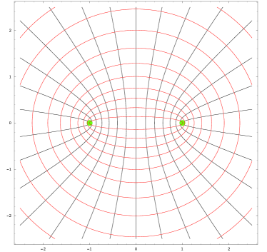
Figure 10: (Color online) Splay rich (hyperbolic) and bend-rich (ellipsoidal) families of nematic ”flow” lines generated by two $s=\frac{1}{2}$ disclinations. The two families of flow lines are the equipotential and field lines of a complex function $\Omega(z)$ whose branch cut is a horizontal line connecting the two defects.

The bond angle of the director oriented along the streamlines is easily extracted from the argument of the complex vector field in Eq.(105), with the result

$$\alpha(x,y)=\arctan\left[\frac{y^{2}+1-x^{2}-\sqrt{(y^{2}+x^{2}+1)^{2}-4x^{2}}}{2xy}\right]\!\!\!\!\!\!\quad.$$ (107)

In this simple example, one can explicitly check that the result in Eq.(107) is recovered through the more familiar route of superposing the solutions corresponding to the two isolated defects

$$\alpha(x,y)=\frac{1}{2}\arctan\left[\frac{y}{x-1}\right]+\frac{1}{2}\arctan\left[\frac{y}{x+1}\right]\!\!\!\!\!\!\quad.$$ (108)

The applicability of the method of conformal mappings to finding liquid crystal textures can be justified by means of simple geometric reasoning. We start by noting that the curl and divergence of a two dimensional vector field $\bf{v}$, whose streamlines and orthogonal trajectories are labelled by the subscripts $s$ and $p$ respectively, can be expressed geometrically via the relations Needham-book

$$\partial_{x}\!\!\!\!\!\quad v_{x}+\partial_{y}\!\!\!\!\!\quad v_{y}\equiv\textbf{$\nabla$}\cdot\textbf{v}=\partial_{s}\!\!\!\!\!\quad|v|+\kappa_{p}\!\!\!\!\!\quad|v|\!\!\quad.$$ (109)

$$\partial_{x}\!\!\!\!\!\quad v_{y}-\partial_{y}\!\!\!\!\!\quad v_{x}\equiv\textbf{$\nabla$}\times\textbf{v}=-\partial_{p}\!\!\!\!\!\quad|v|+\kappa_{s}\!\!\!\!\!\quad|v|\!\!\quad,$$ (110)

where $\kappa_{s}$ and $\kappa_{p}$ are the respective curvatures while $\partial_{s}$ and $\partial_{p}$ are the directional derivatives along the two orthogonal families of level curves. The direction of increasing $p$ is chosen to make a counterclockwise $\frac{\pi}{2}$ angle with $\bf{v}$. For example the black lines in Fig. 10 trace the electric field $\bf{v}$ generated by a uniformly charged plate or the flow lines of an ideal fluid exiting a slit of width given by the branch cut. Unlike the liquid crystal director in Eq.(105), the magnitude of $\bf{v}$ is allowed to vary with position. By construction, such a vector field is divergence free and curl free, hence

$$\kappa_{s}=\partial_{p}\log|v|\!\!\quad,$$ (111)

$$\kappa_{p}=-\!\!\!\!\quad\partial_{s}\log|v|\!\!\quad.$$ (112)

By combining Equations (111) and (112), we obtain the geometric condition that a family of equipotential lines (or streamlines) needs to satisfy in order to be identified as level curves of an harmonic potential, namely

$$\frac{\partial\kappa_{p}}{\partial p}+\frac{\partial\kappa_{s}}{\partial s}=0\!\!\quad.$$ (113)

This condition is entirely cast in terms of the curvatures of the equipotential lines and streamlines without explicit reference to either the potential to be assigned or to the magnitude of the vector field $\textbf{v}(z)$ Bive92 ; Need94 . This is a natural language to discuss orientational order in liquid crystals since the director $\vec{n}(z)$ is a vector field of unit magnitude.

If we take the liquid crystal director to form a constant angle with respect to $\textbf{v}(z)$, the curvatures $\kappa_{s}$ and $\kappa_{p}$ in Eq.(113) can be simply cast as the directional derivatives of $\alpha$ along the streamlines and equipotential lines respectively. In fact, the curvature of these contour lines is the rate of change of their directions which is naturally parameterized by $\alpha$. Hence Eq.(113) reduces to

$$\frac{\partial^{2}\alpha}{\partial p^{2}}+\frac{\partial^{2}\alpha}{\partial^{2}s}=0\!\!\quad.$$ (114)

The left hand side of Eq.(117) is the Laplacian of $\alpha$ expressed in terms of orthogonal coordinates along $s$ and $p$. Since the Laplacian is coordinate independent, Eq.(114) is equivalent to Eq.(101) and $\alpha(x,y)$ represents (apart from an arbitrary global rotation) the desired texture that minimizes the Frank free energy when $K_{1}=K_{3}$.

As a byproduct, Equations (111) and (112) can help to visualize how the elastic energy stored in every portion of the texture of Fig. 10 is distributed between bend and splay deformations. For most liquid crystals $K_{3}>K_{1}$, so the texture with director tangent to the streamlines will be energetically favored (black lines in Fig. 10). In this case, the full Frank energy density can be rewritten in terms of the local curvatures of streamlines and equipotential lines via the simple relation

$$K_{3}\!\!\!\!\quad(\textbf{$\nabla$}\times\textbf{n})^{2}+K_{1}\!\!\!\!\quad(\textbf{$\nabla$}\cdot\textbf{n})^{2}=K_{3}\!\!\!\!\quad{\kappa_{s}}^{2}+K_{1}\!\!\!\!\quad{\kappa_{p}}^{2}\!\!\quad.$$ (115)

The energetically costly deformation involving bend takes place only around the defects in a region of radius of the order of their separation. Elsewhere $\kappa_{s}$ is vanishingly small. In contrast, $\kappa_{p}$ drops off more slowly at large distances like the inverse of the radius of a circle centered on the midpoint between the two disclinations. Splay deformations are present throughout the system but they have a smaller energy cost $K_{1}$. The converse situation occurs if $K_{3}<K_{1}$ so that the texture represented by the red equipotential lines in Fig. 10 becomes energetically favored.

The curvatures $\kappa_{s}$ and $\kappa_{p}$ are respectively the real and imaginary parts of the complex curvature, $K(z)=\kappa_{s}+i\kappa_{p}$, of the mapping. This quantity can be readily derived from the complex potential $\Omega(z)$. For calculational purposes, it is more convenient to recast Eq.(116) in the form $\kappa_{p}+i\kappa_{s}=-\frac{|\Omega^{\prime}|\!\!\!\!\!\quad\Omega^{\prime\prime}}{\Omega^{\prime 2}}$.

$$K(z)\equiv\kappa_{s}+i\kappa_{p}=-i\!\!\!\!\!\quad\frac{|\Omega^{\prime}|\!\!\!\!\!\quad\overline{\Omega^{\prime\prime}}}{\overline{\Omega^{\prime}}\!\!\!\!\!\quad^{2}}\!\!\quad.$$ (116)

The reader is referred to the mathematical literature Bive92 ; Needham-book for a proof of Eq.(116). The intuitive significance of the complex curvature can be grasped by considering how a conformal mapping $f=\Omega^{-1}$ acts on a curve with local curvature $\kappa$ at a point in the $z=x+iy$ plane. The curve is mapped onto an image curve in the $w=u+iv$ plane whose curvature $\kappa^{\prime}$ at the corresponding point differs from $\kappa$. The curvature $\kappa^{\prime}$ of the image curve is determined by two mechanisms. Firstly, the mapping $f(z)$ locally stretches distances by a factor $|f^{\prime}(z)|$, hence the radius of curvature of the image curve will be naturally multiplied by this amplifying factor. The second mechanism arises because a conformal mapping can introduce curvature even if none was originally present (in the isothermal net) simply by locally twisting the direction of the isothermal net by an angle equal to $\arg\!\!\!\!\quad[f^{\prime}(z)]$. For this reason, the complex derivative $f^{\prime}(z)$ is sometimes called an amplitwist and encodes information on the local effect of the mapping Needham-book . The non-analytic function $K(z)$ controls the amount of curvature generated ex-novo by the mapping. For example, the mapping $f(z)=Cos(z)$ transforms a grid of horizontal lines (think of them as a possible direction for the nematic molecules in the defect-free ground state) into the family of hyperbolae in Fig. 10 corresponding to a defected texture with two $+1/2$ disclinations. It is not surprising that the free energy density stored in the defected texture is simply proportional (in the one Frank constant approximation) to

$$\left(\frac{\partial\alpha}{\partial p}\right)^{2}+\left(\frac{\partial\alpha}{\partial s}\right)^{2}=\kappa_{s}^{2}+\kappa_{p}^{2}=|K(z)|^{2}\!\!\quad,$$ (117)

where the two elastic constants were set to be equal in Eq.(115) and the director $\textbf{n}(z)$ was parameterized in terms of the bond angle $\alpha(z)$. The Frank free energy is thus proportional to the complex curvature modulus-squared in analogy with the Helfrich free energy of a membrane whose derivation rests on an higher dimensional generalization of Eq.(115).

Appendix C Vibrational spectrum of colloidal molecules

In this appendix we provide an introduction to the group theoretical treatment of the vibrational spectrum of colloidal ”molecules”. The more complicated cases of hexatic (p=6) and tetratic (p=4) order are analyzed in some detail (see Fig. 11).

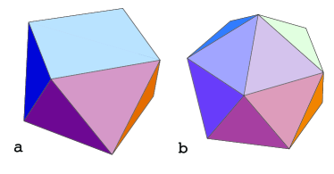
Figure 11: (a) The ground state of a tetratic phase exhibits eight short disclination lines located at the vertices of a square antiprism inscribed in the sphere. (b) The twelve disclination that characterize hexatic order s sphere lie at the vertices of an icosahedron.

The starting point of the group theoretical treatment of the vibrational spectrum of colloidal ”molecules” is the observation that the defects displacements from equilibrium, q (see Eq.(45), form the basis of a $reducible$ representation of the point group of the molecule. If a molecule is acted upon by a symmetry operation, a new configuration will result in which the displacements of each defect will be permuted and transformed, but inter-defect distances and angles will be preserved. Here we take the point of view that the defects themselves are not permuted only their displacements, for example defect $i$ may exchange its displacement coordinates $q_{i}$ with defect $j$. The liquid crystal free energy (in the one Frank constant approximation) is therefore invariant under all the operations of the point group of the colloidal defect array.

The action of each operation of the group is naturally represented by a distinct $2N\times 2N$ matrix ($N$ is the number of defects) that relates the new and old defect positions. This representation can be completely reduced by choosing a set of symmetry-related normal coordinates that are obtained from the original ones by means of a linear transformation. When normal coordinates are used, the matrixes representing the action of the symmetry group can be brought in block diagonal form simultaneously. Energetically degenerate linear combination of the original coordinates form the smallest sets invariant under application of any symmetry operation of the group. The members of any one set generate an $irreducible$ representation of the group.

Table 2: Character for the irreducible representations of the icosahedral point group together with the character of the twenty-four-dimensional representation $\Upsilon$ generated by the defect displacements.

$Y$	$E$	12$C_{5}$	12$C^{2}_{5}$	20$C_{3}$	15$C_{2}$
$A$	1	1	1	1	1
$F_{1}$	3	$\tau$	$-\!\!\!\!\quad\tau^{-1}$	0	$-1$
$F_{2}$	3	$-\!\!\!\!\quad\tau^{-1}$	$\tau$	0	$-1$
$G$	4	$-1$	$-1$	1	0
$H$	5	0	0	$-1$	1
$Y$	24	$2\tau^{-1}$	$-2\tau$	0	0

For each point group there is only a small number of inequivalent irreducible representations generally classified by the characters of their transformations. The characters of the transformations are simply defined as the traces of the matrices corresponding to each symmetry operation and they are conveniently tabulated in most texts of group theory WilsonDeciusCross-book ; Landau-quantum-book (see Tables 1-3 for the character tables relevant to the tetrahedral, icosahedral and twisted-cube shaped distributions of defects on a sphere).

The task of finding the number of degenerate eigenmodes, $n^{(\gamma)}$, with a given symmetry (labelled by $\gamma$) reduces to counting how many times the corresponding irreducible representation appears in a reducible representation. Note that the characters of the original representation are the same as the ones of the completely reduced one since the two differ only by a change of coordinates which preserves the trace. Thus, the character $\chi_{R}$ of the completely reduced representation will be the sum of the characters of the various irreducible representations that it contains

$$\chi_{R}=\sum_{\gamma}n^{(\gamma)}\chi_{R}^{(\gamma)}\!\!\quad,$$ (118)

where $\chi_{R}^{(\gamma)}$ labels the character of the symmetry operation $R$ in the irreducible representation $\gamma$. By appealing to the orthogonality of the characters one can write an expression for $n^{(\gamma)}$ in analogy with the familiar expression for the component of a vector along a given basis axis WilsonDeciusCross-book ; Landau-quantum-book

$$n^{(\gamma)}=\frac{1}{g}\sum_{R}\chi_{R}^{(\gamma)\ast}\!\!\!\!\!\quad\chi_{R}\!\!\quad,$$ (119)

where $g$ is the number of the symmetry operations in the group and $\chi_{R}$ is the character of the completely reduced representation. Eq.(119) is equivalent to Eq.(49) quoted in the main text, as long as the sum over the group elements $R$ is replaced by a weighted sum over the classes in the group since the characters of group elements in the same class are equal.

We now adopt the analysis of Ref.WilsonDeciusCross-book ; Landau-quantum-book to provide a set of rules that produce the characters $\chi_{R}$ of the reducible representation generated by the coordinates without working out the full form of the transformation matrices. There are two key points to notice. First only the defects located on a symmetry axis or plane contribute to $\chi_{R}$ the trace of the transformation matrix; defects whose displacements are instead interchanged or permuted by the symmetry operation contribute only to the non-diagonal terms of the matrix and hence can be ignored in determining the character $\chi_{R}$. Second the directions along which the displacements from equilibrium are measured can be chosen freely since the trace is invariant upon coordinate transformations. It is generally convenient to choose them so that only one of the two displacements components is affected by the symmetry operation.

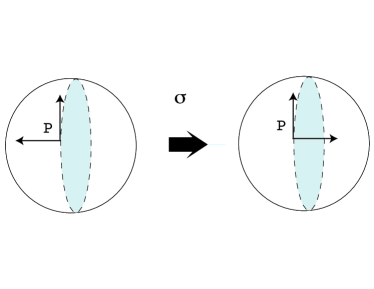
Figure 12: Schematic illustration of the inversion through an equatorial plane of symmetry (shaded circle bisecting a sphere) for a reflection $\sigma$. The longitudinal displacement of the defect is unchanged while the direction of the latitudinal one is inverted.

As a simple example, consider a defect lying on a reflection plane (see Fig. 12). The displacement vectors before and after the symmetry operation is applied are $\{\delta\theta,\delta\phi\}$ and $\{\delta\theta,-\delta\phi\}$ respectively. The resulting contribution to the character from a single defect is thus $1-1=0$. Inversions through a center of symmetry (coinciding with the center of the sphere) have a vanishing contribution to $\chi_{R}$ because there are no defects there that can contribute to $\chi_{R}$.

A rotation $C_{n}^{k}$ by an angle $\frac{2\pi k}{n}$ through an n-fold axis of symmetry on which the defect lies leads to the following transformation laws for the longitudinal and latitudinal displacements

$$\left(\begin{array}[]{c}\delta\theta_{i}\!\!\!\!\!\quad^{\prime}\\ \\ \delta\phi_{i}\!\!\!\!\!\quad^{\prime}\\ \end{array}\right)=\left(\begin{array}[]{cc}\cos\left(\frac{2\pi k}{n}\right)&-\sin\left(\frac{2\pi k}{n}\right)\\ \\ \sin\left(\frac{2\pi k}{n}\right)&\cos\left(\frac{2\pi k}{n}\right)\\ \end{array}\right)\left(\begin{array}[]{c}\delta\theta_{i}\\ \\ \delta\phi_{i}\\ \end{array}\right)\!\!\quad.$$ (120)

We measure displacements using polar coordinates with respect to the symmetry axis; the prime denotes the orthogonal displacements after the symmetry operation $C_{n}^{k}$ is applied. Inspection of Eq.(120) shows that the contribution from $C_{n}^{k}$ to the character $\chi_{R}$ is equal to $2\cos\left(\frac{2\pi k}{n}\right)$ times the number of defects lying on the axis of rotation. On the other hand the contribution to $\chi_{R}$ from the improper rotation $S^{k}_{n}$ is zero. To see this note that the symmetry operation $S^{k}_{n}$ is a rotary reflection achieved by performing a successive rotation through an (alternating) axis followed by a reflection in the plane perpendicular to the axis $k$ times. An example of a molecule possessing the symmetry operation $S_{4}$ is methane, CH₄, with the carbon atom lying at the intersection between an alternating axis and the reflection plane (See Fig. 5-2 in Ref. WilsonDeciusCross-book ). The tetrahedral defect configuration considered in this paper does not posses any defect at the position occupied by the carbon atom of the methane molecule. More generally, the possibility of having a defect whose equilibrium position is unchanged by the rotary reflection is ruled out because such defect would have to lie off the spherical surface at the intersection between the alternating axis and the plane of reflection.

To sum up, each of the characters, $\chi_{R}$, of the completely reduced representation formed by the displacement coordinates is given by the number of atoms whose equilibrium positions are not changed by the symmetry operation $R$ times its fundamental character as derived in the previous paragraphs. Similar results that apply to unconstrained molecules whose atoms have three dimensional displacements are listed in Table 6-1 of Ref. WilsonDeciusCross-book . The resulting characters for the tetrahedral, icosahedral and tilted cube defects configurations are listed in Tables 1-3.

Table 3: Character for the irreducible representations of the tilted cube point group together with the character of the sixteen-dimensional representation $\Xi$ generated by the defect displacements.

$D_{4d}$	$E$	2$S_{8}$	2$C_{4}$	2$S^{3}_{8}$	$C_{2}$	4$C^{1}_{2}$	4$\sigma_{2}$
$A_{1}$	1	1	1	1	1	1	1
$A_{2}$	1	1	1	1	1	$-1$	$-1$
$B_{1}$	1	$-1$	1	$-1$	1	$1$	$-1$
$B_{2}$	1	$-1$	1	$-1$	1	$-1$	$1$
$E_{1}$	2	$\sqrt{2}$	0	$-\sqrt{2}$	$-2$	$0$	$0$
$E_{2}$	2	$0$	$-2$	$0$	2	$0$	$0$
$E_{3}$	2	$-\sqrt{2}$	$0$	$\sqrt{2}$	$-2$	$0$	$0$
$\Xi$	16	0	0	0	0	0	0

Upon using Eq.(49) and the character table 2 we can decompose the 24 dimensional representation, $Y$, formed by the displacements from an icosahedral equilibrium configuration into irreducible representations. The result reads

$$Y=2H+2G+2F_{1}\!\!\quad.$$ (121)

The three rigid body rotations correspond to one of the two triplets in $F_{1}$ while the remaining 21 independent normal coordinates form energetically degenerate multiplets with the following degeneracy factors: 2 quintets, 2 quartets and 1 triplet. This analysis is confirmed upon direct diagonalization of the representation $Y$ which leads the 21 non-vanishing eigenvalues $\lambda_{i}$, with the multiplicities shown bold in parenthesis

$$\lambda_{i}=\{0.87\!\!\!\!\!\!\!\quad\times(\textbf{5}),\!\!\!\!\!\quad 0.09\!\!\!\!\!\!\!\quad\times(\textbf{5}),$$

$$\!\!\!\!\!\quad 0.74\!\!\!\!\!\!\!\quad\times(\textbf{4}),\!\!\!\!\!\quad 0.22\!\!\!\!\!\!\!\quad\times(\textbf{4}),\!\!\!\!\!\quad 0.96\!\!\!\!\!\!\!\quad\times(\textbf{3})\}\!\!\quad.$$ (122)

Note that the normal modes in the second quintet are much ”softer” than the rest.

A similar analysis applied to the twisted cube configuration of defects leads to the following decomposition of the (defects’ displacements) representation, $\Xi$,

$$\Xi=2E_{1}+2E_{2}+2E_{3}+A_{1}+A_{2}+B_{1}+B_{2}\!\!\quad.$$ (123)

where the three rigid body rotations are contained in one of the two doublets $E_{3}$ and in the singlet $A_{2}$, which leaves five doublets and three singlets for the eigenvalues $\zeta_{i}$. Direct diagonalization of $\Xi$ leads four doublets, one triplet and two singlets of non-vanishing eigenvalues,

$$\zeta_{i}=\{1.37\!\!\!\!\!\!\!\quad\times(\textbf{3}),\!\!\!\!\!\quad 1.31\!\!\!\!\!\!\!\quad\times(\textbf{2}),\!\!\!\!\!\quad 0.89\!\!\!\!\!\!\!\quad\times(\textbf{2}),$$

$$\!\!\!\!\!\quad 0.47\!\!\!\!\!\!\!\quad\times(\textbf{2}),\!\!\!\!\!\quad 0.06\!\!\!\!\!\!\!\quad\times(\textbf{2}),\!\!\!\!\!\quad 0.11,\!\!\!\!\!\quad 1.26\}$$ (124)

The discrepancy between the degeneracies found by direct diagonalization on one hand and group theory on the other is caused by an accidental symmetry of the potential energy of the tilted-cube arrangement of defects. Hence the first triplet is to be interpreted as the missing doublet and singlet that happen to have the same energy even if there is no symmetry reasons to expect so. The modes in the last doublet of Eq.(124) are the softest.

References

- (1) P. G. de Gennes and J. Prost, The Physics of Liquid Crystals (Clarendon Press, Oxford, 1993).
- (2) M. Kleman and O. D. Lavrentovich Soft matter physics (Springer, New York, 2003).
- (3) M. Kleman Points, Lines and walls (Wiley, New York, 1983).
- (4) R. D. Kamien, Science 299, 1671 (2003).
- (5) D. R. Nelson, Nano. Lett. 2, 1125 (2002).
- (6) R. A. Segalman, A. Hexemer, R. C. Hayward, and E. J. Kramer, Macromolecules 36, 3272 (2003).
- (7) M. Park, C. Harrison, P. M. Chaikin, R. A. Register, D. H. Adamson, Science 276, 1401 (1997).
- (8) R. D. Kamien, Rev. Mod. Phys. 74, 953 (2002).
- (9) O. D. Lavrentovich, Liq. Cryst. 24, 117 (1998).
- (10) G. P. Crawford and S. Zumer, Liquid Crystals in Complex Geometries (Francis and Taylor, London,1996).
- (11) D. R. Nelson, Phys. Rev. B 28, 5515 (1983).
- (12) F. C. MacKintosh and T. C. Lubensky, Phys. Rev. Lett. 67, 1169 (1991).
- (13) T. C. Lubensky and J. Prost, J. Phys. II (France), 2, 371 (1992).
- (14) M. J. Bowick, D. R. Nelson and A. Travesset, Phys. Rev. B. 62, 8738 (2000).
- (15) A. R. Bausch, M. J. Bowick, A. Cacciuto, A. D. Dinsmore, M. F. Hsu, D. R. Nelson, M. G. Nikolaides, A. Travesset and D. A. Weitz, Science 299, 1716 (2003).
- (16) M. Bowick, D. R. Nelson and A. Travesset, Phys. Rev. E. 69, 041102 (2004).
- (17) V. Vitelli and D. R. Nelson, Phys. Rev. E. 70, 051105 (2004).
- (18) V. Vitelli and A. M. Turner, Phys. Rev. Lett. 93, 215301 (2005).
- (19) J. M. Park and T. C. Lubensky, Phys. Rev. E 53, 2648 (1996).
- (20) P. Lenz and D. R. Nelson, Phys. Rev. E 67, 031502 (2003).
- (21) D. R. Nelson and L. Peliti, J. Phys. 48, 1085 (1987).
- (22) F. David, E. Guitter and L. Peliti, J. Phys. 48, 2059 (1987).
- (23) F. David, in Statistical Mechanics of Membranes and Surfaces, edited by D. R. Nelson et al., (World Scientific, Singapore, 2004).
- (24) S. Weinberg, Gravitation and Cosmology, (Wiley, New York, 1972).
- (25) S. Chandrasekhar, Liquid Crystals (Cambridge University Press, Cambridge, 1994).
- (26) F. Dyson, private communication.
- (27) V. I. Smirnov, A course of Higher Mathematics, vol. 3 part 2 (Pergamon Press, Oxford, 1964).
- (28) T. Needham, Visual Complex Analysis (Oxford University Press, Oxford, 1997).
- (29) E. B. Wilson, J. C. Decius and P. C. Cross, Molecular Vibrations (Dover, New York, 1955).
- (30) E. M. Lifshitz and L. D. Landau, Quantum Mechanics: Non-Relativistic Theory (Butterworth-Heinemann, Oxford, 1977).
- (31) C. Chiccoli, I. Feruli, O. D. Lavrentovich, P. Pasini, S. V. Shiyanovskii and C. Zannoni, Phys. Rev. E 66, 030701(R) (2002).
- (32) H. Stark, Phys. Rep. 351, 387 (2001).
- (33) T. C. Lubensky, D. Pettey, N. Currier and H. Stark, Phys. Rev. E 57, 610 (1998).
- (34) P. Poulin, H. Stark, T. C. Lubensky and D. A. Weitz, Science 275, 1770 (1997).
- (35) H. W. Wyld, Mathematical Methods for Physics (Perseus Books, Reading, 1999), pp. 272-276.
- (36) I. S. Gradstein and I. M. Ryshik, Tables of series, products and integrals (Verlag Harri, Deutsch, Frankfurt, 1981).
- (37) R. P. Feynman, R. B. Leighton and M. Sands, The Feynman Lectures on Physics, vol. 2, (Addison-Wesley, Reading, 1963).
- (38) B. A. Ovrut and S. Thomas, Phys. Rev. D 43, 1314 (1991).
- (39) I. C. Bivens, Math. Mag. 65, 226 (1992).
- (40) T. Needham, Math. Mag. 67, 92 (1994).