Thermo-Statistical description of the Hamiltonian non extensive systems
The reparametrization invariance

Abstract

In the present paper we continue our reconsideration about the foundations for a thermostatistical description of the called Hamiltonian nonextensive systems. After reviewing the selfsimilarity concept and the necessary conditions for the ensemble equivalence, we introduce the reparametrization invariance of the microcanonical description as an internal symmetry associated with the dynamical origin of this ensemble. Possibility of developing a geometrical formulation of the thermodynamic formalism based on this symmetry is discussed, with a consequent revision about the classification of phase-transitions based on the concavity of the Boltzmann entropy. The relevance of such conceptions are analyzed by considering the called Antonov isothermal model.

I Introduction

As alsewhere discussed, the study of the non extensive systems constitutes an interesting and fascinating challenger for the developments of the Thermodynamics and Statistical Mechanics bog ; bec ; sol ; lyn ; pie ; pos ; kon ; tor ; gro1 ; ato ; kud ; par ; stil ; sta1 . An important feature of this kind of systems is the existence of long-range correlations, whose origin delays on the existence of long-range interactions among the constituents particles or the small (or mesoscopic) nature of the system.

We address in our previous paper vel.self a reconsideration of the foundations for a thermo-statistical description of the special case of the nonextensive Hamiltonian systems. The main conclusions derived from this work are the following: (1) The universality of the microscopic mechanism of chaoticity supports the generic applicability of a thermostatistical description with microcanonical basis for the nonintegrable many-body Hamiltonian systems Kolmogorov ; Arnold ; Moser ; PF1 ; PF2 ; arnold , even for those nonextensive systems with long-range interactions pettini4793 ; pettini 51 ; pet ; cohenG , (2) Extensive conditions of the traditional systems are not longer applicable for the nonextensive systems, but such properties could be generalized by considering the scaling selfsimilarity concept vel.self which is considered in order to establish an adequate thermo-statistical description in this context.

We will continue in the present paper our analysis of the foundations for a thermo-statistical description of the nonextensive Hamiltonian systems. Our aim now is to show how the scaling selfsimilarity concept could be used in order to perform an appropriate thermodynamic formalism in the systems with long-range interactions. As already discussed in our previous work, most of the Hamiltonian systems with a practical interest exhibit exponential selfsimilarity scaling laws vel.self . This is the reason why the present discussion will be focussed in this special class of the nonextensive Hamiltonian systems. Interested reader could also review a similar approach to the one developed in this work in ref. velTsal for the case of the potential selfsimilarity scaling laws, which seem to be associated with the popular Tsallis nonextensive statistics tsal .

II Reviewing selfsimilarity

Selfsimilarity is just a general symmetry of the macroscopic description exhibited under the scaling transformations of the system size in $\alpha$ times, $N\rightarrow N\left(\alpha\right)=\alpha N$, which manifests itself in every macroscopic behavior of the system, even in the macroscopic dynamics vel.self . From the mathematical viewpoint, selfsimilarity appears as a multiplicative uniparametric group of transformations $T_{\alpha}$, $T_{\alpha}T_{\beta}=T_{\alpha\beta}$, which acts on those fundamental macroscopic observables $I$ determining the microcanonical macroscopic state of a given system, leading in this way to a scaling transformation of the number of microscopic configurations $W=W\left(I\right)$ (microcanonical accessible phase-space volume) whose form does not depend on the macroscopic state and can be represented as follows:

$$I\left(\alpha\right)=T_{\alpha}I\Rightarrow W\left[\alpha\right]=\mathcal{Y}\left\langle\alpha\mathcal{Y}^{-1}\left(W\right)\right\rangle,$$ (1)

where the function $\mathcal{Y}\left(x\right)$ determines what we refer as the selfsimilarity scaling law of the system. According to the framework developed in the previous work vel.self , the selfsimilarity scaling law $\mathcal{Y}\left(x\right)$ determines the generalized Boltzmann Principle (microcanonical entropy) and the specific statistical entropic compatible with the selfsimilatity of a given system:

$$S_{B}^{\mathcal{L}}=\mathcal{L}\left(W\right)\Leftrightarrow S_{e}^{\mathcal{L}}=\sum_{k}p_{k}\mathcal{L}\left(\frac{1}{p_{k}}\right),$$ (2)

where $\mathcal{L}\left(x\right)=\mathcal{Y}^{-1}\left(x\right)$. Such definitions should be considered as the starting point in the generalization of the traditional thermodynamic formalism.

Two remarkable cases of selfsimilarity scaling laws are the exponential selfsimilarity:

$$\mathcal{Y}\left(x\right)=\exp\left(x\right)\Rightarrow S_{BG}=-\sum_{k}p_{k}\ln p_{k},$$ (3)

which leads to the usual Boltzmann-Gibbs statistics, and the potential selfsimilarity:

$$\mathcal{Y}\left(x\right)=\exp_{q}\left(x\right)\Rightarrow S_{q}=-\sum_{k}p_{k}^{q}\ln_{q}p_{k},$$ (4)

associated with the Tsallis nonextensive statistics tsal , where $\ln_{q}x=\exp_{q}^{-1}\left(x\right)=\left(x^{1-q}-1\right)/\left(1-q\right)$, is the q-generalized logarithmic function. Among them, the most extended in practical applications is the exponential selfsimilarity scaling laws (3). Extensivity of traditional systems is just a special case of this kind of scaling selfsimilarity, whose scaling selfsimilarity transformations obey the well-kown form:

$$\left.\begin{array}[c]{c}N\left(\alpha\right)=\alpha N\\ E\left(\alpha\right)=\alpha E\\ V\left(\alpha\right)=\alpha V\end{array}\right\}\Rightarrow W\left(\alpha\right)=\exp\left(\alpha\ln W\right).$$ (5)

While a generic Hamiltonian system of the form:

$$H\left(q,p\right)=\sum_{ij}\frac{1}{2}a^{ij}p_{i}p_{j}+V\left(q\right),$$ (6)

with the total potential energy $V\left(q\right)$, $i,j=1,2,\ldots n$ and $q=\left(q^{1},q^{2},\ldots q^{n}\right)$, exhibits an exponential growing of the microcanonical accessible phase-space volume $W$ with the increasing of the system degrees of freedom $n$ vel.self , supporting in this way an exponential growing of $W$ during the scaling operation $n\rightarrow n\left(\alpha\right)=\alpha n$, the selfsimilarity scaling transformations $T_{\alpha}$ acting on the fundamental macroscopic observables (such as the total energy $E$ or the systems volume $V$) are far to look like the extensive case (5) in the long-range interacting systems.

A very simple example of system with nontrivial scaling transformations is found for the selfgravitating gas of identical nonrelativistic particles with a finite incompressible volume $v$ which interact among them by means of the Newtonian gravity. Obviously, the particles density $\rho$ in this system obeys the inequallity $\rho\leq\rho_{0}=1/v$. For very low energies and large densities where $\rho\sim\rho_{0}$ the scaling transformations are approximately given by:

$$N\left(\alpha\right)=\alpha N,~{}E\left(\alpha\right)\simeq\alpha^{\frac{5}{3}}E,V\left(\alpha\right)\simeq\alpha V,$$ (7)

while for very high energies and low densities where the particles size can be dismissed since $\rho\ll\rho_{0}$, such scaling transformations can be expressed asyntotically as follows:

$$N\left(\alpha\right)=\alpha N,~{}E\left(\alpha\right)\simeq\alpha^{\frac{7}{3}}E,V\left(\alpha\right)\simeq\alpha^{-1}V,$$ (8)

results which have been obtained in refs.velastro ; chava12 and it will be shown again in the section V.

Generally speaking, the determination of the specific selfsimilarity scaling transformations $T_{\alpha}$ could be a very difficult task because of there is no methodology to establish them in a given application outside the extensive context. As already suggested in the introductory section of our previous paper vel.self , systems with long-range interactions look like the extensive systems in the neighborhood of the second-order phase transitions due to the long-range correlations existing in this region. This is the reason why we think that the well-known Renormalization Group methods Gold should play a crucial role in the determination of the scaling selfsimilarity of a given nonextensive system.

III Thermodynamic formalism

As elsewhere discussed, the thermodynamic formalism is based on the equivalence in the thermodynamic limit $N\rightarrow\infty$ between the microcanonical ensemble $\hat{\omega}_{M}$ and the canonical ensemble $\hat{\omega}_{BG}$ gallavotti :

$$\hat{\omega}_{M}=\frac{1}{\Omega\left(I,N\right)}\delta\left\langle I-\hat{I}_{N}\right\rangle,~{}\hat{\omega}_{BG}=\frac{1}{Z\left(\beta,N\right)}\exp\left(-\beta\hat{I}_{N}\right),$$ (9)

derived from the consideration of the Maximal Entropy Principle jaynes by using the extensive entropy (3), where $\hat{I}_{N}$ are all those macroscopic observables (integrals of motion) determining the macroscopic state. Obviously, the thermodynamic limit $N\rightarrow\infty$ is equivalent to carry out a scaling transformation $T_{\alpha}$ on the observables $I$ with $\alpha\rightarrow\infty$.

The ensemble equivalence can be shown by considering the Laplace transformation which relates their partition functions:

$$Z\left(\beta,N\right)=\int e^{-\beta I}\Omega\left(I,N\right)dI.$$ (10)

Introducing the Boltzmann entropy $S_{B}\left(I,N\right)=\ln W$, where $W=\Omega\delta I$, and the Planck thermodynamic potential $\mathcal{P}\left(\beta\right)=-\ln Z\left(\beta\right)$, the Laplace transformation could be rewritten as follows:

$$\exp\left\langle-\mathcal{P}\left(\beta,N\right)\right\rangle=\int\exp\left\langle-\left[\beta I-S_{B}\left(I,N\right)\right]\right\rangle\frac{dI}{\delta I}.$$ (11)

We immediately recognize in the argument of the exponential function the well-known Legendre transformation between the thermodynamic potentials:

$$\mathcal{P}_{m}\left(\beta_{m},N\right)=\beta_{m}I-S_{B}\left(I,N\right),\text{ with }\beta_{m}=\frac{\partial S_{B}}{\partial I},$$ (12)

where the subindex $m$ means that such quantities are associated with the microcanonical description.

It can be shown by using the steepest descend method that the equivalence between $\mathcal{P}_{m}\left(\beta_{m},N\right)$ and $\mathcal{P}\left(\beta,N\right)$ takes place in the thermodynamic limit when the following conditions are applicable:

• The macroscopic observables $I$ behave in a extensive-like way during the selfsimilarity scaling transformation $T_{\alpha}$:

  $$T_{\alpha}I=\alpha I\Rightarrow S_{B}\left(T_{\alpha}I,\alpha N\right)=\alpha S_{B}\left(I,N\right).$$ (13)

• There is only one stationary point $i_{s}=I/N$ satisfying the relation:

  $$\beta=\frac{\partial s_{B}\left(i_{s}\right)}{\partial i},$$ (14)

  where $s_{B}\left(i\right)=\frac{1}{N}S_{B}\left(iN,N\right)$ is the entropy per particle.

The condition i) is only trivially satisfied by the extensive systems when the microcanonical description is performed by using the called extensive observables, i.e. total energy, electric charge, etc. However, extensivity does not take place in systems with long-range interactions. In this context extensivity should be substituted by the scaling selfsimilarity, but the extensive-like character (13) of the macroscopic observables $I$ does not hold generally speaking.

The condition ii) demands the concavity of the Boltzmann entropy, property which can not be everywhere satisfied. The existence of several stationary points leads to a catastrophe in the Legendre transformation which is related with the occurrence of first-order phase transitions at a given value of $\beta$. Such anomaly appears in those regions where at least one eigenvalue of the Hessian of the Boltzmann entropy:

$$k_{nm}=\frac{\partial^{2}s_{B}}{\partial i^{n}\partial i^{m}},$$ (15)

is positive. As already shown by Gross, every anomaly in the Hessian of the Boltzmann entropy can be related with the existence of phase transitions, extending in this way the identification of such critical phenomena is systems outside the thermodynamic limit gro1 .

IV Reparametrization invariance

We will show in this section that the conditions i) and ii) could be satisfied by considering the called reparametrization invariance of the microcanonical description. ¿What is such reparametrization invariance? As already commented, the microcanonical ensemble is just a dynamical ensemble, and therefore, every symmetry of the microscopic dynamics is also relevant at the macroscopic level in the microcanonical description. The reparametrization invariance is just a symmetry with a dynamical origin.

IV.1 Mathematical definition and Physical meaning

Let us consider now all those integrals of motion $\hat{I}\left(X\right)=\left\{I^{1}\left(X\right),I^{2}\left(X\right),\ldots I^{n}\left(X\right)\right\}$ determining the microcanonical thermostatistical description of a given nonintegrable many-body Hamiltonian system. Each admissible value of the above set integrals of motion $I=\left\{I^{1},I^{2},\ldots I^{n}\right\}$ determine certain subset $\mathcal{S}_{p}$ of the phase-space $\mathcal{X}$ :

$$X\in\mathcal{S}_{p}\equiv\left\{X\in\mathcal{X}\left|I^{k}\left(X\right)=I^{k},k=1,2,\ldots n\right.\right\}.$$ (16)

in which is enclose the system microscopic dynamics in a given microcanonical macroscopic state.

The totality of these admissible ”points” $\left\{I\right\}$ defines a subset $\mathcal{R}_{I}$ of the n-dimensional Euclidean space $\mathcal{R}^{n}$, while the totality of the corresponding phase-space subsets $\left\{\mathcal{S}_{p}\right\}$ defines certain partition $\Im\left(\mathcal{X}\right)$ of the phase-space $\mathcal{X}$:

$$\Im\left(\mathcal{X}\right)=\left\{\mathcal{S}_{p}\subset\mathcal{X}\left|~{}{\displaystyle\bigcup_{p}}\mathcal{S}_{p}=\mathcal{X}~{};~{}\mathcal{S}_{p}\cap\mathcal{S}_{q}=\varnothing\right.\right\}.$$ (17)

The above definitions (16) and (17) allow the existence of certain bijective map $\psi_{I}$ between the elements of $\Im\left(\mathcal{X}\right)$ (subsets $\mathcal{S}_{p}\subset\mathcal{X}$) and the elements of $\mathcal{R}_{I}$ (points $I\in\mathcal{R}^{n}$)

$$\psi_{I} :\Im\left(\mathcal{X}\right)\rightarrow\mathcal{R}_{I}\equiv\left\{\forall\mathcal{S}_{p}\in\Im\left(\mathcal{X}\right)~{}\exists I\in\mathcal{R}_{I}\subset\mathcal{R}^{n}\right.$$

$$\left|\forall X\in\mathcal{S}_{p}\Rightarrow I^{k}\left(X\right)=I^{k},k=1,2,\ldots n\right\}.$$ (18)

The bijective character of this map provides to the partition $\Im\left(\mathcal{X}\right)$ the same topological features of certain subset $\mathcal{R}_{I}$ of the n-dimensional Euclidian space $\mathcal{R}^{n}$. Now on we refer the partition $\Im\left(\mathcal{X}\right)$ as the abstract space of the integrals of motions, and it will be denoted simply by $\Im$. We say that the map $\psi_{I}$ defines a n-dimensional Euclidean coordinate representation $\mathcal{R}_{I}$ of the abstract space $\Im$.

The coordinate representation $\mathcal{R}_{I}$ of $\Im$ is not unique. Let $\mathcal{R}_{I}$ and $\mathcal{R}_{\varphi}$ be two diffeomorphic subsets of the n-dimensional Euclidean space $\mathcal{R}^{n}$, that is, there exist a diffeomorphic map:

$$\varphi:\mathcal{R}_{I}\rightarrow\mathcal{R}_{\varphi}\equiv\left\{\forall I\in\mathcal{R}_{I}~{}\exists\varphi\in\mathcal{R}_{\varphi}\left|\det\left(\frac{\partial\varphi^{j}}{\partial I^{k}}\right)\not=0\right.\right\},$$ (19)

among their elements. The terms ”diffeomorphic map” means that the n-dimensional Euclidean subsets $\mathcal{R}_{I}$ and $\mathcal{R}_{\varphi}$ posses the same topological and diffeomorphic (differential) structure. The map $\psi_{\varphi}=\psi_{I}o\varphi^{-1}$ defines a new bijective application among the elements of the space $\Im$ and the points $\varphi\in\mathcal{R}_{\varphi}$, $\psi_{\varphi}:$ $\Im\rightarrow\mathcal{R}_{\varphi}$, and consequently, $\psi_{\varphi}$ is also another n-dimensional Euclidean coordinate representation of $\Im$. The coordinate representations $\mathcal{R}_{I}$ and $\mathcal{R}_{\varphi}$ are equivalent because of they represent the same abstract space $\Im$.

Generally speaking, a reparametrization change is carried out when we move from the Euclidean representation $\mathcal{R}_{I}$ towards an equivalent Euclidean representation $\mathcal{R}_{\varphi}$. The totality of the diffeomorphic maps (19) constitutes certain group of transformations called the group of diffeomorphisms of the space $\Im$, $Diff\left(\Im\right)$, which is the maximal symmetry that a geometrical theory could exhibit.

Every reparametrization change (19) also induces a reparametrization of the integrals of motions $\varphi\Rightarrow\varphi_{X}$:

$$\varphi_{X}:\hat{I}\left(X\right)\rightarrow\hat{\varphi}\left(X\right)\equiv\left\{\varphi^{1}\left\langle\hat{I}\left(X\right)\right\rangle,\ldots\varphi^{n}\left\langle\hat{I}\left(X\right)\right\rangle\right\},$$ (20)

Since $\hat{I}\left(X\right)$ are integrals of motions, every $\varphi^{k}\left\langle I\left(X\right)\right\rangle\in$ $\hat{\varphi}\left(X\right)$ will be also a integral of motion. Due to the bijective character of the reparametrization change $\varphi:\mathcal{R}_{I}\rightarrow\mathcal{R}_{\varphi}$, the new set of integrals of motion $\hat{\varphi}\left(X\right)$ generates the same partition $\Im\left(\mathcal{X}\right)$ of the phase-space. This is the reason why the sets $\hat{I}\left(X\right)$ and $\hat{\varphi}\left(X\right)$ can be considered as equivalent representations of the relevant integrals of motion determining the microcanonical description.

Since the totality of the phase-space points belonging to a given subset $\mathcal{S}_{p}\in$ $\Im\left(\mathcal{X}\right)$ represents the same microcanonical macroscopic state, and the diffeomorphic and topological structure of the abstract space $\Im$ does not depend on the reparametrization changes, it is not difficult to understand that the microcanonical description is reparametrization invariant.

Theorem 1

The microcanonical ensemble $\hat{\omega}_{M}$ (9) is invariant under every reparametrization change $\varphi:\mathcal{R}_{I}$ $\rightarrow\mathcal{R}_{\varphi}$.

Proof. Such invariance is straightforward derived from the following identity of the Dirac delta function:

$$\delta\left\langle\varphi\left(I\right)-\varphi\left(\hat{I}_{N}\right)\right\rangle=\left|\frac{\partial\varphi}{\partial I}\right|^{-1}\delta\left\langle I-\hat{I}_{N}\right\rangle,$$ (21)

which leads to the following transformation rule for the partition function $\Omega$:

$$\Omega\left(\varphi;N\right)=\left|\frac{\partial\varphi}{\partial I}\right|^{-1}\Omega\left(I;N\right),$$ (22)

and consequently:

$$\frac{1}{\Omega\left(\varphi,N\right)}\delta\left\langle\varphi-\hat{\varphi}_{N}\right\rangle =\frac{1}{\Omega\left(I,N\right)}\delta\left\langle I-\hat{I}_{N}\right\rangle,$$

$$\hat{\omega}_{M}\left(\varphi,N\right) =\hat{\omega}_{M}\left(I,N\right).$$ (23)

We have considered here the implicit dependence of integrals of motion on the system size $N$.   

A corollary of the Theorem 1 is that the Physics derived from the microcanonical description is reparametrization invariant since the expectation values of every macroscopic observable $\hat{O}$ derived from the microcanonical distribution function $\hat{\omega}_{M}$ exhibits this kind of symmetry:

$$\bar{O}=\int\hat{O}\hat{\omega}_{M}dX\Rightarrow\bar{O}\left(\varphi,N\right)=\bar{O}\left(I,N\right),$$ (24)

relation which is straightforwardly followed by using the identity (23).

The reparametrization invariance does not introduce anything new in the macroscopic description except the possibility of describing the macroscopic state by using any representation $\mathcal{R}_{\varphi}$ equivalent to the original representation $\mathcal{R}_{I}$, a situation analogue to describe the physical space $\mathcal{R}^{3}$ by using a Cartesian coordinates $\left(x,y,z\right)$ or spherical coordinates $\left(r,\theta,\varphi\right)$.

Notice that the diffeomorphic reparametrization changes demand the analyticity of the integrals of motions, which is a necessary condition for a particular integral of motion $\hat{I}^{k}$ be relevant in the macroscopic description. On the other hand, the integrals of motions $\hat{I}$ are derived from their commutativity with the Hamiltonian $\hat{H}$. Since $\hat{H}$ is one of those integrals of motion determining the macroscopic state (total energy), the Hamiltonian loses its identity during the reparametrization changes (20). The only way to preserve the condition $\left\{\hat{H},\hat{I}\right\}=0$ during the reparametrization changes is by demanding the commutativity among all those integrals of motion determining the macroscopic state $\left\{\hat{I}^{k},\hat{I}^{l}\right\}\equiv 0$:

$$\left\{\hat{\varphi}^{i},\hat{\varphi}^{j}\right\}=\sum_{kl}\frac{\partial\varphi^{i}}{\partial I^{k}}\frac{\partial\varphi^{j}}{\partial I^{l}}\left\{\hat{I}^{k},\hat{I}^{l}\right\}\equiv 0.$$ (25)

Interestingly, this is the necessary condition for the simultaneous determination of physical observables in the Quantum Mechanics, and therefore, reparametrization invariance is also consistent in this level.

IV.2 Some geometrical aspects

Reparametrization invariance is a symmetry of the microcanonical description which allows us to perform a geometrical description in this framework, a covariant formulation of the Thermostatistics. Geometrical formulations of the Thermostatistics are very well-known in Physics. Some recently proposed geometrical formulations are given in refs. gro1 and rupper ; topH2 .

A very important question is to determine the transformation rules of the physical observables and the thermodynamical function under the reparametrization changes. Now on the Einstein summation convention will be assumed. As already shown, the microcanonical distribution function and the physical observables behave as scalar functions during the reparametrization changes:

$$\hat{\omega}_{M}\left(\varphi,N\right)=\hat{\omega}_{M}\left(I,N\right),~{}\bar{O}\left(\varphi,N\right)=\bar{O}\left(I,N\right).$$ (26)

The transformation rule microcanonical partition function $\Omega$ corresponds with the transformation rule of a scalar tensorial density:

$$\Omega\left(\varphi,N\right)=\left|\frac{\partial\varphi}{\partial I}\right|^{-1}\Omega\left(I,N\right).$$ (27)

The first derivatives of a given physical observable $\bar{O}$ behave as the components of a covariant vector:

$$\frac{\partial\bar{O}}{\partial\varphi^{m}}=\frac{\partial I^{k}}{\partial\varphi^{m}}\frac{\partial\bar{O}}{\partial I^{k}}\sim\upsilon_{m}=\frac{\partial I^{k}}{\partial\varphi^{m}}\upsilon_{k}.$$ (28)

The transformation rule of the second-order tensors is given by:

$$A_{mn}=\frac{\partial I^{k}}{\partial\varphi^{m}}\frac{\partial I^{l}}{\partial\varphi^{n}}A_{kl}.$$ (29)

However, such covariant second-order tensor cannot be obtained by differentiation without the introduction of a Riemannian structure, that is, without introducing a Riemannian metric.

The microcanonical partition function $\Omega$ allows us the introduction of the invariant measure $d\mu=\Omega dI$. Taking into account such invariant measure, the integration of a given physical observable $\bar{O}$ defined on the space $\Im$ (microcanonical ensemble) is directly related with the phase-space integration:

$${\displaystyle\int\limits_{\Sigma}}\bar{O}d\mu\equiv{\displaystyle\int\limits_{\Sigma\left(\mathcal{X}\right)}}O\left(X\right)dX,$$ (30)

where $\Sigma$ is a subset of the space $\Im$, and $\Sigma\left(\mathcal{X}\right)$ is its corresponding image in the phase-space.

Strictly speaking, the Boltzmann entropy $S_{B}=\ln W$ is not an scalar function. The microcanonical accessible volume $W$ is just the invariant measure of a small neighborhood $\Sigma$ of the interest point obtained after by performing a coarsed grained partition of the space $\Im$:

$$W=\mu\left(\Sigma\right)={\displaystyle\int\limits_{\Sigma}}d\mu.$$ (31)

In applications $W$ is taken approximately by $W\simeq\Omega\delta I$, where the volume $\delta I$ of the coarsed grain subset $\Sigma$ is regarded as a very small constant. The small constant $\delta I$ becomes unimportant when $N$ is very large, that is, with the imposition of the thermodynamic limit, and consequently, the Boltzmann entropy could be considered as a scalar function in this limit.

IV.3 Consequences of this dynamical symmetry on the thermodynamic formalism

The microcanonical ensemble provides a full characterization of the macroscopic properties of a given isolate Hamiltonian system in thermodynamic equilibrium. The imposition of the thermodynamic limit $N\rightarrow\infty$ leads under certain conditions to the equivalence of the microcanonical description with certain simplified characterization: the macroscopic description performed by the canonical ensemble. As already discussed, such canonical ensemble is determined from the relevant statistical entropy derived from the specific scaling selfsimilarity exhibited by the interest system, i.e.: the exponential selfsimilarity is associated with the Shannon-Boltzmann-Gibbs extensive entropy (3), which naturally leads to the called Boltzmann-Gibbs distributions (9).

It is very easy to verify that the canonical distribution function (9) does not exhibit the original reparametrization invariance of the microcanonical ensemble. This means that the Physics in the canonical ensemble depends on the coordinate representation $\mathcal{R}_{I}$ of the abstract space $\Im$ of the relevant integrals of motion used for perfoming the macroscopic characterization of a given system. Therefore, the thermodynamic formalism could not satisfy this kind of symmetry, and consequently, the ordering information derived from its consideration is not reparametrization invariant.

As already discussed in section III, the equivalence between the microcanonical and the canonical descriptions demands the fulfillment the conditions i) and ii), and therefore, such ensemble equivalence could not be performed by using an arbitrary representation. However, the existence of the reparametrization invariance of the microcanonical descriptions plays a crucial role in arriving to a well-defined thermodynamic formalism.

The extensive-like behavior of the integrals of motion under the scaling transformations is simply satisfied by chosing an appropriate coordinate representation $\mathcal{R}_{\varphi}$ of the space $\Im$ exhibiting this kind of behavior under the scaling transformations. There are some trivial examples in which this demand is very easy to accomplish. Considering the example illustrated at the end of section II, the total energy of the selfgravitating gas of identical point particles interacting by means of the Newtonian gravity grows with the scaling following a $\alpha^{\frac{7}{3}}$ power law velastro , and therefore, an appropriate representation with an extensive-like behavior could be $\varphi=N\varphi\left(E/E_{0}\right)$, where $E_{0}=GM^{2}/R$ is the characteristic constant energy which evidently follows the same $\alpha^{\frac{7}{3}}$ power law, being $\varphi\left(x\right)$ a bijective function.

The reader may notice that such procedure differs from the called Kac argument kac because of the total energy is not arbitrarily forced to be extensive, since its scaling behavior is determined from the system selfsimilarity. We only demand the extensivity in the coordinate representation of the relevant integrals of motion in order to ensure the ensemble equivalence in the thermodynamic limit. The main difficulty in chosing an appropriate representation of the relevant integrals of motion is that the specific selfsimilarity scaling transformation $T_{\alpha}$ acting on the space $\Im$ is a priori unknown and have to be determined.

As already shown, the transition from the microcanonical towards the canonical description with the imposition of the thermodynamic limit and the consequent establishment of the system selfsimilarity leads to a breakdown of the original reparametrization symmetry. However, ¿is the reparametrization invariance completely broken during this transition? The answer is no. This fact is very easy to understand by considering the above example about the selfgravitating gas: anyone bijective function $\varphi=N\varphi\left(E/E_{0}\right)$ could be used with the purpose of describing the macroscopic characterization, and therefore, there is a complete set of admissible coordinate representations $\mathcal{C}=\left\{\mathcal{R}_{\varphi}\right\}$ exhibiting an extensive-like behavior during the scaling transformations.

Let $\mathcal{R}_{I}$ and $\mathcal{R}_{\varphi}$ be two coordinate representations belonging to the set of admissible representations $\mathcal{C}$ and $\varphi=\psi_{\varphi}o\psi_{I}^{-1}:\mathcal{R}_{I}\rightarrow\mathcal{R}_{\varphi}$, the reparametrization change between them. Since the scaling transformations for every coordinate in both representations are given by $T_{\alpha}^{k}\left(I\right)=\alpha I^{k}$ and $T_{\alpha}^{m}\left(\varphi\right)=\alpha\varphi^{m}$, the reparametrization change $\varphi\left(I\right)$ is a homogeneous map satisfying the relations:

$$\varphi^{m}\left(\alpha I\right)=\alpha\varphi^{m}\left(I\right)\Leftrightarrow\varphi^{m}\left(I\right)=I^{k}\frac{\partial\varphi^{m}\left(I\right)}{\partial I^{k}},$$ (32)

for $m=1,2,\ldots n$.

The complete set of reparametrization changes acting in the set of admissible representations $\mathcal{C}$ constitutes the Group of Homogeneous transformations $\mathcal{H}$, which is a subgroup of the Group of diffeormorphisms $Diff\left(\Im\right)$ already commented. The symmetry associated with the transformations of the Homogeneous group $\mathcal{H}$ is just the residual symmetry of the original reparametrization invariance of the microcanonical description.

Theorem 2

The thermodynamic potential $\mathcal{P}_{m}$ obtained from the Legendre transformation (12) is $\mathcal{H}$-invariant:

$$\mathcal{P}_{m}=I^{k}\frac{\partial S_{B}\left(I\right)}{\partial I^{k}}-S_{B}\left(I\right)=\varphi^{m}\frac{\partial S_{B}\left(\varphi\right)}{\partial\varphi^{m}}-S_{B}\left(\varphi\right).$$ (33)

Proof. The demostration is straightforwardly followed by performing a variable change in the partial derivative of the Boltzmann entropy:

$$I^{k}\frac{\partial S_{B}}{\partial I^{k}}=I^{k}\left(\frac{\partial\varphi^{m}}{\partial I^{k}}\frac{\partial S_{B}}{\partial\varphi^{m}}\right)=\left(I^{k}\frac{\partial\varphi^{m}}{\partial I^{k}}\right)\frac{\partial S_{B}}{\partial\varphi^{m}},$$ (34)

and considering the homogeneous character of the reparametrization change (32):

$$I^{k}\frac{\partial S_{B}}{\partial I^{k}}\equiv\varphi^{m}\frac{\partial S_{B}}{\partial\varphi^{m}}.$$ (35)

 

We have shown in this way that the ”microcanonical” thermodynamic functions $S_{B}$ and $\mathcal{P}_{m}$, as well as their first derivatives exhibit a covariant behavior under the reparametrizations changes of the Homogeneous group $\mathcal{H}$. However, it does not mean that the thermodynamic formalism exhibits this kind of symmetry because of the conditions ii) is necessary to satisfy also in order to ensure the ensemble equivalence. The fulfillment of this condition could be perturbed because of the reparametrization changes can affect the concavity of the Boltzmann entropy. Let us to illustrate this by considering the following example.

Let $\varphi$ be a map between two seminfinite Euclidean lines, $\varphi:\mathcal{R}^{+}\rightarrow\mathcal{R}^{+}$, which in the representation $\mathcal{R}_{x}$ is given by the concave function $\varphi\left(x\right)=\sqrt{x}$ (where $x>0$). Let us now consider a reparametrization change $\psi:\mathcal{R}_{x}\rightarrow\mathcal{R}_{y}$ given by $y=x^{\frac{1}{4}}$ (which is evidently bijective). The map $\varphi$ in the new representation $\mathcal{R}_{y}$ is given by the function $\varphi\left(y\right)=y^{2}$ (where $y>0$), which clearly is a convex function.

The above trivial example teaches us that the concavity of the Boltzmann entropy depends on the representation $\mathcal{R}_{I}\in\mathcal{C}$ used to perform the canonical description, and therefore, ensemble equivalence (or inequivalence) depends on the coordinate representation of the space $\Im$. This is a very interesting point since the ensemble inequivalence is a signature of the first-order phase transitions.

According to the Microcanonical Thermostatistics of Gross gro1 , the Hessian of the Boltzmann entropy (15) gives a complete characterization of the phase-transitions in the microcanonical ensemble. However, in spite of the aparent similarity, the components of the Hessian are not the components of a covariant tensor of second-order because of they obey the transformation rule:

$$\frac{\partial^{2}S_{B}}{\partial\varphi^{m}\partial\varphi^{n}}=\frac{\partial I^{k}}{\partial\varphi^{m}}\frac{\partial I^{l}}{\partial\varphi^{n}}\frac{\partial^{2}S}{\partial I^{k}\partial I^{l}}+\frac{\partial^{2}I^{k}}{\partial\varphi^{m}\partial\varphi^{n}}\frac{\partial S}{\partial I^{k}},$$ (36)

while the correct transformation rule is given by (29). This means that such classification of phase-transitions based on the concavity of the entropy is not reparametrization invariant. Therefore, the coordinate representation of the space $\Im$ should be specified in order to precise the existence of first-order phase transitions. How such ambiguity in the first-order phase-transition existence could be physically acceptable?

The question is that the coordinate representation $\mathcal{R}_{I}$ of the space $\Im$ is determined from the external constrains imposed to the system. This idea is very easy to understand analysing the case of the extensive systems. Ordinarily, canonical ensemble $\omega_{BG}=Z^{-1}\left(\beta\right)\exp\left(-\beta E\right)$ is experimentally implemented by putting the interest system in a thermal contact with a heat bath. This experimental arrangement not only fix the system temperature $T=\beta^{-1}$, but also the coordinate representation by using the system energy $E$. Thus, the existence of first-order phase transition is not necessarily an intrinsic characteristic of a given system because of it depends on the external conditions which have been imposed.

What happen when the ensemble inequivalence or any other anomaly is present at a given point $p\in$ $\Im$ without matter the coordinate representation $\mathcal{R}_{I}\in\mathcal{C}$ used in the macroscopic description? Such anomalies are not representation-dependent, that is, they do not depend on the external conditions imposed to the system. These kind of anomalies are intrinsic characteristic of the system, and consequently, they have a topological character. A anomaly of this kind reflects the ocurrence of considerable changes in the microscopic picture of an isolate Hamiltonian system, i.e.: an ergodicity breaking Gold .

This idea brings us the recently proposed hypothesis about the topological origin of the phase-transitions topH2 . According to the ideas developed by these authors, the origin of the chaoticity of the microscopic dynamics and the origin of the phase transitions at the macroscopic level delay on the geometrical and topological structure of the configurational space. We think that such abrupt topological changes in the configurational space could be took place when they are associated with topological anomalies at the macrocopic level, that is, when such anomalies are not dependent of the coordinate representation of the space $\Im$. The non correspondence between topological changes and phase transitions observed in ref.ana might be explained due to the non topological character of such phase-transitions. The following theorem establishes the non existence of topological ensemble inequivalences in those systems controlling by only one scaling invariant parameter $\varepsilon$, $T_{\alpha}\left(\varepsilon\right)=\varepsilon$.

Theorem 3

Let $s\left(\varepsilon\right)$ be the entropy per particle of a given system which is controlled by only one scaling invariant variable $\varepsilon$. Let us also suppose that the second derivative of $s\left(\varepsilon\right)$ exists, being $s\left(\varepsilon\right)$ a convex function in the interval $\varepsilon_{1}<\varepsilon<\varepsilon_{2}$, and a concave function elsewhere. There is a reparametrization change $\varphi:\mathcal{R}_{\varepsilon}\rightarrow\mathcal{R}_{\varphi}$ in which the entropy $s$ becomes a concave function.

Proof. The transformation rule of the second derivative of the entropy during the reparametrization change $\varphi:\mathcal{R}_{\varepsilon}\rightarrow\mathcal{R}_{\varphi}$ is given by:

$$\frac{\partial^{2}s}{\partial\varphi^{2}}=\left(\frac{\partial\varepsilon}{\partial\varphi}\right)^{2}\frac{\partial^{2}s}{\partial\varepsilon^{2}}+\frac{\partial^{2}\varepsilon}{\partial\varphi^{2}}\frac{\partial s}{\partial\varepsilon}.$$ (37)

Considering the auxiliary function $a\left(\varepsilon\right)$:

$$\frac{\partial^{2}s}{\partial\varphi^{2}}=-\left(\frac{\partial\varepsilon}{\partial\varphi}\right)^{2}a\left(\varepsilon\right),$$ (38)

the first derivative of the bijective map $\varphi\left(\varepsilon\right)$ could be rewritten as follows:

$$\frac{\partial\varphi\left(\varepsilon\right)}{\partial\varepsilon}=C\beta\left(\varepsilon\right)\exp\left(\int\frac{a\left(\varepsilon\right)d\varepsilon}{\beta\left(\varepsilon\right)}\right),$$ (39)

where $C$ is certain positive integration constant and $\beta\left(\varepsilon\right)=\partial s\left(\varepsilon\right)/\partial\varepsilon$. The entropy $s$ will be a concave function in the new coordinate representation $\mathcal{R}_{\varphi}$ whenever $a\left(\varepsilon\right)>0$. This demand is very easy to satisfy by considering:

$$a\left(\varepsilon\right)=\left\{\begin{array}[c]{cc}\partial^{2}s\left(\varepsilon\right)/\partial\varepsilon^{2}&\text{wherever }s\left(\varepsilon\right)\text{ be convex}\\ -\partial^{2}s\left(\varepsilon\right)/\partial\varepsilon^{2}&\text{wherever }s\left(\varepsilon\right)\text{ be concave}\end{array}\right.,$$ (40)

which directly leads to the following bijective map:

$$\frac{\partial\varphi\left(\varepsilon\right)}{\partial\varepsilon}=\left\{\begin{array}[c]{cc}C_{1}&\varepsilon<\varepsilon_{1}\\ C_{2}\beta^{2}\left(\varepsilon\right)&\varepsilon_{1}<\varepsilon<\varepsilon_{2}\\ C_{3}&\varepsilon>\varepsilon_{2}\end{array}\right.,$$ (41)

where we have considered here the possibility of introducing a different values for integration constant $C$ in different regions. By choosing $C_{1}=1$, $C_{2}=1/\beta^{2}\left(\varepsilon_{1}\right)$ and $C_{3}=\beta^{2}\left(\varepsilon_{2}\right)/\beta^{2}\left(\varepsilon_{1}\right)$, we not only ensure the concavity of the entropy, but also the continuity of the first and second derivatives of the bijective map $\varphi\left(\varepsilon\right)$.   

The analysis about the existence of topological ensemble inequivalences for two or more controlling variables is an open problem. While topological ensemble inequivalence are not present in the unidimensional case, they are not the only topological anomalies presents in this context. The existence of a discontinuity in the first derivative of the entropy in the thermodynamic limit is a example of anomaly which could not be avoided by a reparametrization change $\varphi\left(\varepsilon\right)$ with a continue first derivative $\partial\varphi\left(\varepsilon\right)/\partial\varepsilon$. Such anomalies have been recently reported in the astrophysical context, and they are usually classified as microcanonical phase-transitions chava.micro . Existence of singularities in the second derivatives of the entropy are also unavoidable by reparametrizations, which are related with the well-known second-order phase transitions appearing due to the existence of an spontaneous symmetry breaking at the microscopic level Gold . Interestingly, the above topological anomalies appear due to an ergodicity breaking in underlying the microscopic dynamics Gold ; chava.micro .

V Astrophysical system

Let us to illustrate the relevance of the scaling selfsimilarity and reparametrization invariance by considering the microcanonical description of a nontrivial nonextensive Hamiltonian system: the selfgravitating gas of identical nonrelativistic point particles interacting throughout the Newtonian gravity:

$$H_{N}=K_{N}+V_{N}=\sum_{i}\frac{1}{2m}\mathbf{p}_{i}^{2}-\frac{1}{2}Gm^{2}\sum_{\left\langle i\not=j\right\rangle}\frac{1}{\left|\mathbf{r}_{i}-\mathbf{r}_{j}\right|}.$$ (42)

The long-range singularity of the gravitational potential will be avoided by enclosing the system in a spherical rigid container of radio $R$. The short-range singularity will be regularized by considering a mean-field approximation. The above conditions leads to the well-known isothermal model of Antonov antonov .

After the integration of the linear momentum variables $\mathbf{p}$’s, the accessibe phase-space volume can be expressed by:

$$W=\delta\varepsilon\frac{1}{N!}\left(\frac{2m\pi}{h^{2}}\right)^{\frac{3}{2}N}\int d^{3N}r\frac{1}{\Gamma\left(\frac{3}{2}N\right)}\left\langle E-V_{N}\left\{r\right\}\right\rangle^{\frac{3}{2}N-1},$$

where $\left\{r\right\}=\left(\mathbf{r}_{1},\mathbf{r}_{2},\ldots\mathbf{r}_{n}\right)$, $d^{3N}r=\prod_{k}d^{3}\mathbf{r}_{k}$, and $\delta\varepsilon$ a very small energy constant. Introducing the characteristics units for the linear dimension $l_{0}=R$, total mass $M=Nm$, and total energy $E_{0}=GM^{2}/R$, and considering a very large system size $N$ in order to consider the Stirling approximation $\Gamma\left(x\right)\simeq\left(x/e\right)^{x}$, the above expression could be rewritten as follows:

$$\frac{1}{N}\ln W\simeq\frac{3}{2}\ln\left\langle C_{0}RN^{\frac{1}{3}}\right\rangle+\ln\omega\left(U\right),$$ (43)

where $C_{0}=4\pi Gm^{3}/3e^{\frac{5}{3}}h^{2}$ and $\omega\left(U\right)$ is given by:

$$\ln\omega\left(U\right)=\lim_{N\rightarrow\infty}\frac{1}{N}\ln\left(\int d^{3N}\xi\left\langle U-V_{N}\left\{\xi\right\}\right\rangle^{\frac{3}{2}N}\right),$$ (44)

being $U=E/E_{0}$ and $\xi=r/l_{0}$. The entropy per particle (43) is scaling invariant under the following scaling selfsimilarity transformations:

$$N\left(\alpha\right)=\alpha N,R\left(\alpha\right)=\alpha^{-\frac{1}{3}}R\Rightarrow E\left(\alpha\right)=\alpha^{\frac{7}{3}}E\text{,}$$ (45)

result supporting the thermodynamic limit:

$$N\rightarrow\infty\text{, keeping fixed }\frac{E}{N^{\frac{7}{3}}}\text{ and }RN^{\frac{1}{3}}$$ (46)

already obtained in refs.velastro ; chava12 . Now on $s_{0}\left(U\right)=\ln\omega\left(U\right)$ will be referred simply as the system entropy.

The progresive calculation of (44) is carried out by considering a mean-field approximation and them using the steepest descend method whose details will be omitted here in the sake of brevity. Such procedure leads to the following min-max problem:

$$s_{0}\left(U\right)\simeq\min_{\mu}\max_{\rho}\left\{\frac{3}{2}\ln\left\langle U-V\left[\rho\right]\right\rangle+s\left[\rho\right]+\mu\left\langle 1-N\left[\rho\right]\right\rangle\right\},$$ (47)

where the functionals $V\left[\rho\right]$ (potential energy), $s\left[\rho\right]$ (local entropy) and $N\left[\rho\right]$ (particle number) are given by:

$$V\left[\rho\right] =-\frac{1}{2}\int d^{3}\mathbf{\xi}d^{3}\mathbf{\xi}^{\prime}\frac{\rho\left(\mathbf{\xi}\right)\rho\left(\mathbf{\xi}^{\prime}\right)}{\left|\mathbf{\xi}-\mathbf{\xi}^{\prime}\right|},~{}N\left[\rho\right]=\int d^{3}\mathbf{\xi}~{}\rho\left(\mathbf{\xi}\right),$$

$$\begin{array}[c]{c}s\left[\rho\right]=\int d^{3}\mathbf{\xi}~{}\left\langle-\rho\left(\mathbf{\xi}\right)\ln\rho\left(\mathbf{\xi}\right)+\rho\left(\mathbf{\xi}\right)\right\rangle.\end{array}$$ (49)

The problem (47) leads to the following Boltzmann distribution for the particles density $\rho$:

$$\rho\left(\mathbf{\xi}\right)=\exp\left\langle-\mu-\beta\varphi\left(\mathbf{\xi}\right)\right\rangle,$$ (50)

where $\beta$ is the canonical parameter:

$$\beta=\frac{\partial\ln\omega\left(U\right)}{\partial U}=\frac{3}{2\left(U-V\right)},$$ (51)

$\mu$, the chemical potential associated with the normalization condition:

$$\int d^{3}\mathbf{\xi}~{}\rho\left(\mathbf{\xi}\right)=1,$$ (52)

and $\varphi\left(\xi\right)$ is the gravitational potential related with $\rho$ throughout the Poisson problem:

$$\Delta\varphi\left(\mathbf{\xi}\right)=4\pi\rho\left(\mathbf{\xi}\right),~{}\varphi\left(1\right)=-1,~{}\varphi^{\prime}\left(1\right)=1.$$ (53)

The equation (51) can be rewritten in order to obtain the caloric curve $U$ versus $\beta$:

$$U=\frac{3}{2\beta}+V\text{, where }V=\frac{1}{2}\int d^{3}\mathbf{\xi}~{}\rho\left(\mathbf{\xi}\right)\varphi\left(\mathbf{\xi}\right).$$ (54)

The solution with spherical symmetry of the above problem is numerically implemented by introducing the function $\Phi\left(\xi\right)=-\mu+\ln\beta-\beta\varphi\left(\xi\right)$, and solving the following Poisson-Boltzmann problem:

$$\frac{1}{\xi^{2}}\frac{\partial}{\partial\xi}\left\langle\xi^{2}\frac{\partial\Phi\left(\xi\right)}{\partial\xi}\right\rangle=-4\pi\exp\left\langle\Phi\left(\xi\right)\right\rangle,$$ (55)

whose boundary conditions at the origin are:

$$\Phi\left(0\right)=\psi,~{}\frac{\partial}{\partial\xi}\Phi\left(0\right)=0,$$ (56)

where $\psi=\ln\left(\beta\rho_{c}\right)$, being $\rho_{c}$ in the central density $\rho_{c}=\rho\left(0\right)$. Thus, the functions $\rho\left(\xi\right)$, $\varphi\left(\xi\right)$ as well as the macroscopic variables and thermodynamic potentials $U$, $\beta$, $\mu$, $s_{0}$ are obtained as functions of the parameter $\psi$, i.e.: $\beta$ and $\mu$ are given by:

$$\Phi\left(1;\psi\right)=-\mu+\ln\beta+\beta,~{}\frac{\partial}{\partial\xi}\Phi\left(1;\psi\right)=-\beta.$$ (57)

Figure 1: Thermostatistical description of the Antonov isothermal model by using the representation $\mathcal{R}_{U}$.

The FIG.1 shows the microcanonical thermostatistical description of the Antonov isothermal model. The caloric curve (panel a) and the central density $\rho_{c}$ versus $U$ dependence (panel b) show the existence of thermodynamical states with a negative heat capacity (branch A-B), as well as the ocurrence of a gravitational collapse $\rho_{c}\rightarrow\infty$ for low energies. The branch A-B-C corresponds to the equilibrium thermodynamic states, while the other branch are just unstable saddle points. According to the caloric curve, there are no equilibrium thermodynamical states when $U<U_{A}=-0.334$ or $\beta>\beta_{B}=2.52$. The ensemble inequivalence in the branch A-B is associated with the convexity of the entropy (panel c) in this region.

As already discussed in our previous paper vel.self , when this model system initially isolate with a total energy $U\in\left(U_{A},U_{B}\right)$ (branch A-B) is put in a thermal contact with a heat bath with $\beta>\beta_{B}$, it becomes unstable developing an isothermal gravitational collapse antonov , so that, the Antonov isothermal model is very sensible the external influence of a heat bath in the branch A-B. Such instability can be associated with the existence of a first-order phase transition from a gaseous phase (with $\rho_{c}$ finite) towards a collapsed one ($\rho_{c}\rightarrow\infty$).

The above thermodynamical description was performed in the $\mathcal{R}_{U}$ representation. According to the Theorem 3, the entropy convexity could be avoided by considering an appropriate reparametrization change. In order to obtain such appropriate representation, let us to observe the $\psi$ versus $U$ dependence also shown in panel d of the FIG.1. It is easy to see that, dismissing the unstable branch, there is a biunivocal correspondence between these macroscopic observables for all relevant equilibrium thermodynamical states. This fact supports that we can obtain an appropriate representation $\mathcal{R}_{\varphi}$ by considering certain experimental arrangement which keeps fixed the observable $\chi=\exp\left(\psi\right)=\beta\rho_{c}$. The map $\varphi:\mathcal{R}_{U}\rightarrow\mathcal{R}_{\varphi}$ can be established by taking into account that $\chi$ is the canonical parameter in the new representation, which is related with $\beta$ by the transformation rule (28):

$$\chi=\exp\left(\psi\right)=\frac{\partial U}{\partial\varphi}\beta\Rightarrow\frac{d\varphi\left(\psi\right)}{d\psi}=\beta\left(\psi\right)\exp\left(-\psi\right)\frac{dU\left(\psi\right)}{d\psi}.$$ (58)

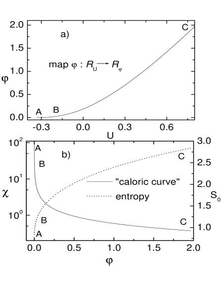
Figure 2: Thermostatistical description of the Antonov isothermal model in the representation $\mathcal{R}_{\varphi}$.

FIG.2 shows the thermostatistical description of the Antonov isothermal model in the representation $\mathcal{R}_{\varphi}$. The reparametrization change $\varphi:\mathcal{R}_{U}\rightarrow\mathcal{R}_{\varphi}$ obtained from the numerical integration of the equation (58) is illustrated in the panel a (which is evidently a bijective map), while the ”caloric curve” $\chi$ versus $\varphi$ and the entropy $s_{0}$ versus $\varphi$ dependence are shown in the panel b. The reader can notice that no ensemble inequivalence takes place in the representation $\mathcal{R}_{\varphi}$, and consequently, the microcanonical description of this model system in the thermodynamic limit becomes equivalent to the one carried out by considering the following ”canonical ensemble”:

$$\hat{\omega}_{B}\left(\chi,N\right)=\frac{1}{Z\left(\chi,N\right)}\exp\left\{-\chi N\varphi\left\langle\frac{1}{E_{0}}H_{N}\right\rangle\right\}$$ (59)

associated with an experimental arrangement which keeps fixed $\chi=\beta\rho_{c}$. Since no ensemble inequivalence is observed, no topological first-order phase transition is present in the Antonov isothermal model.

It is very important to realize that the thermostatistical description obtained from the numerical integration of the Poisson-Boltzmann problem (55) makes use (in an implicit way) of the above ”canonical ensemble” since the spatial functions $\rho$ and $\varphi$, as well as the thermodynamic variables and potentials are obtained as functions of the parameter $\psi=\ln\chi$.

VI Conclusions

We have shown in the present work that an appropriate thermostatistical description of the nonextensive Hamiltonian systems could be performed by considering their scaling selfsimilarity properties as well as the reparametrization invariance of the microcanonical description.

As already discussed in previous sections, the reparametrization invariance is just an internal symmetry of the microcanonical description appearing as a consequence of its dynamical origin. This symmetry allows us to satisfy the necessary conditions i) and ii) (see in section III) for the ensemble equivalence in the thermodynamic limit $N\rightarrow\infty$, and the consequent well-defined character of the thermodynamic formalism based on the Legendre transformation (12) among the thermodynamic potentials. The consideration of the reparametrization invariance makes possible the developing of a geometrical thermodynamic formalism in which the ordering information based on the concavity of the Boltzmann entropy could be defined in a topological fashion, suggesting in this way a new vision of the phase transition concept which seems to be related with the called Topological Hypothesis about the topological origen of the phase transitions topH2 .

Our analysis of the Antonov isothermal model shows the relevance of the selfsimilarity and the reparametrization invariance in the context of the astrophysical systems. An interesting remark derived from this study is that the reparametrization invariance could be used as a powerful tool in order to extend a canonical-like description (59) for those thermodynamical states with a negative heat capacity, fact which leads to a natural improvement of the well-known montecarlo methods based on the consideration of the canonical weight $\exp\left(-\beta E\right)$ yuki . A very important problem is still open: A methodology to derive the relevant scaling selfsimilarity in a given application. Omitting some exceptional cases like the Antonov problem reconsidered in the present paper, derivation of the selfsimilarity scaling transformations is a very difficult task which demands an extension of the Renormalization Group methods Gold .

References

- (1) B. M. Boghosian, Phys. Rev. E 53 (1996) 4754.
- (2) C. Beck, G. S. Lewis, and H. L. Swinney , Phys. Rev. E 63 (2001) 035303.
- (3) T. H. Solomon, E.R. Weeks, and H. L. Swinney, Phys. Rev. Lett. 71 (1993) 3975.
- (4) D. Lynden-Bell , Physica A 263 (1999) 293.
- (5) F. Sylos Labini, M. Montuori and L. Pietronero, Phys. Rep. 293 (1998) 61.
- (6) L. Milanovic, H. A.Posch and W. Thirring, Phys. Rev. E 57 (1998) 2763.
- (7) H. Koyama and T. Konishi, Phys. Lett. A 279 (2001) 226.
- (8) A. Torcini and M. Antoni, Phys. Rev. E 59 (1999) 2746.
- (9) D.H.E Gross, Microcanonical thermodynamics: Phase transitions in Small systems, 66 Lectures Notes in Physics, (World scientific, Singapore, 2001).
- (10) M. Schmidt et al, Phys. Rev. Lett. 86 (2001) 1191.
- (11) A. Kudrolli and J. Henry, Phys. Rev. E 62 (2000) 1489.
- (12) G. Parisi, Physica A 280 (2000) 115.
- (13) P.G. Benedetti and F.H. Stillinger, Nature 410 (2001) 259.
- (14) G.M. Viswanathan , V. Afanasyev , S.V. Buldyrev, E.J. Murphy, and H.E. Stanley, Nature 393 (1996) 413.
- (15) L. Velazquez and F. Guzman, Thermo-Statistical description of the nonextensive Hamiltonian Systems: The selfsimilarity scaling laws, e-print (2006) [cond-mat/0604290].
- (16) A. N. Kolmogorov, Dokl. Akad. Nauk. SSSR 98 (1954).
- (17) V. I. Arnold, Izv. Akad. Nauk. SSSR Ser. Math. 25 (1961).
- (18) J. Moser, Am. Math. Soc. Mem. 81 (1968) 1.
- (19) H. Poincare, Les methodes nouvelles de la mecanique celeste, (Gauthier-Villars, Paris, 1892).
- (20) E. Fermi, Nuovo Cimento 25 (1923) 267; ibidem 26 (1923) 105.
- (21) V.I. Arnold, Mathematical Methods of Classical Mechanics (Springer-Verlag, 1980).
- (22) M. Pettini, Phys. Rev. E 47 (1993) 828.
- (23) M. Cerruti-Sola and M. Pettini, Phys. Rev. E 51 (1995) 53; Phys. Rev. E 53 (1996) 179.
- (24) P. Cipriani and M. Pettini, Astrophys. Space Sci. 283 (2003) 347; e-print (2001) [astro-ph/0102143].
- (25) G. Gallavotti, E.G.D. Cohen, Phys. Rev. Lett. 74 (1995) 2694 ; J. Stat. Phys. 80 (1995) 931.
- (26) L. Velazquez and F. Guzman, Phys. Rev. E 65 (2002) 046134.
- (27) C. Tsallis, J. Stat. Phys. 52 (1988) 479.
- (28) L. Velazquez and F. Guzman, Phys. Rev. E 68 (2003) 066116.
- (29) P. H. Chavanis and I. Ispolatov, Phys. Rev. E 66 (2002) 036109.
- (30) N. Goldenfeld, Lectures on phase transitions and critical phenomena, Frontiers in physics 85, (Perseus Books Publishing, L.L.C., 1992).
- (31) G. Gallavotti, Statistical Mechanics, (Springer, Berlin, 1999).
- (32) E. T. Jaynes, Phys Rev. 106 (1957) 620; ibid 118 (1961) 171; Papers on probability, statistics and statistical physics, edited by R. D. Rosenkrantz (Reidel, Derdrecht, Holland, 1983).
- (33) G. Ruppeiner, Rev. Mod. Phys. 67 (1995) 605.
- (34) L. Casetti, E.G.D. Cohen, and M. Pettini, Phys. Rev. E 65 (2002) 036112.
- (35) M. Kac, G.E. Uhlenbeck and P.C. Hemmer, J. Math. Phys. 4 (1963) 216.
- (36) S. Risau-Gusman, A. C. Ribeiro-Teixeira, D. A. Stariolo, Topology, phase transitions and the spherical model, e-print (2005) [cond-mat/0508419].
- (37) P.H. Chavanis, Phys. Rev. E 65 (2002) 056123.
- (38) V.A. Antonov, Vest. leningr. gos. Univ. 7 , 135 (1962).
- (39) Y. Iba, Int. J. Mod. Phys. C 12 (2001) 623.