From urn models to zero-range processes: statics and dynamics

Abstract

The aim of these lecture notes is a description of the statics and dynamics of zero-range processes and related models. After revisiting some conceptual aspects of the subject, emphasis is then put on the study of the class of zero-range processes for which a condensation transition arises.

Introduction

The models discussed in these notes are simplified models of physical reality. Yet, besides the fact that they play an important role in the elucidation of conceptual problems of statistical mechanics and probability theory, they are instrumental in the understanding of a variety of complex physical situations.

The aim of these notes is a description of the statics and dynamics of zero-range processes (ZRP) [1] and of related models. We present a review of the subject, coming back on some of its conceptual aspects. We restrict all discussions to homogeneous models where all sites are equivalent. Before commencing, we summarise in a few words the main organisation of the text.

In Part I: Statics (sections 1-6), we first show that ZRP are special members of a class of stochastic processes which have the property that their stationary measures are known and have a product structure. The probability of a configuration of the system is given by the Boltzmann formula for an equilibrium urn model with independent sites. Reversibility (for symmetric dynamics) and pairwise balance (for asymmetric dynamics) are inherently related to the structure of the stationary measure. Generalisations to multiple-species ZRP are then addressed. The properties of the stationary measure of ZRP leading to a phase transition between a fluid phase and a condensed phase are finally briefly reviewed, as a preparation for the second part of these notes.

The stochastic nature of ZRP is fully revealed by the study of their dynamics. This is the subject of Part II (sections 7-9). We first address the nonstationary dynamical behaviour of the system when it evolves from a random initial disordered configuration to its stationary state. Then we investigate some aspects of its stationary dynamics, when the system fluctuates in its stationary state. In both cases the model used is that giving rise to condensation.

Part I: Statics (sections 1-6)

1 Dynamical urn models and zero-range processes

1.1 Dynamical urn models

We name dynamical urn model (DUM) the following stochastic process. Consider a finite connected graph, made of $M$ sites (or urns), on which $N$ particles are distributed. The occupation $N_{i}(t)$ of site $i$ ($i=1,\dots,M$) is a random variable, and the total number of particles

$$\sum_{i=1}^{M}N_{i}(t)=N$$

is conserved in time. The model is defined by dynamical rules describing how particles hop from site to site. An elementary step of the dynamics consists in choosing a departure site $d$ and an arrival site $a$ connected to site $d$, and in transferring one of the particles present on site $d$ to site $a$. This process takes place with rate $W_{k,l}$ per unit time, depending on the occupations both of the departure site, $k=N_{d}\neq 0$, and of the arrival site, $l=N_{a}$.

On the complete graph (i.e., in the mean-field geometry), all sites are connected, i.e., sites $d$ and $a$ are chosen independently at random. On finite-dimensional lattices, site $a$ is chosen among the first neighbours of site $d$. In one dimension, site $a$ is chosen to be the right neighbour of site $d$ with probability $p$, or its left neighbour with probability $q=1-p$. In the following we consider the one-dimensional symmetric dynamics, corresponding to $p=1/2$, and the general asymmetric one, corresponding to $p\neq 1/2$, both with periodic boundary conditions.

A configuration of the system is specified by the occupation numbers $N_{i}(t)$, i.e., a complete knowledge of its dynamics involves the determination of $\mathcal{P}(N_{1,}N_{2},\ldots,N_{M})$, the probability of finding the system in a given configuration at time $t$.

The process can be pictorially viewed in terms of colonies and migration. The sites are the colonies, or cities. An individual leaves its colony for another one, with a rate $W_{k,l}$ which depends on the number of members present in both the departure and the arrival colonies. Thus, for example, the philanthrope is characterized by a rate decreasing with $k$ and increasing with $l$, the misanthrope by the converse.

1.2 Zero-range processes

Zero-range processes are just particular cases of DUM, with the additional restriction that the rate $W_{k,l}$ only depends on the occupation of the departure site:

$$W_{k,l}=u_{k}.$$

This simple restriction is enough to lead to a remarkable property of the stationary probability [1, 2]. Indeed, the probability of a configuration of the system is equal to

$${\cal P}(N_{1},\dots,N_{M})=\frac{1}{Z_{M,N}}\prod_{i=1}^{M}p_{N_{i}},$$ (1.1)

where it is understood that $\sum N_{i}=N$, and where the factor $p_{k}=p_{N_{i}=k}$ satisfies the relation

$$u_{k}\,p_{k}=p_{k-1},$$ (1.2)

which leads to the explicit form

$$p_{0}=1,\qquad p_{k}=\frac{1}{u_{1}\dots u_{k}}.$$ (1.3)

The normalisation factor, hereafter refered to as the partition function, reads

$$Z_{M,N}=\sum_{N_{1}}\cdots\sum_{N_{M}}\,p_{N_{1}}\cdots p_{N_{M}}\;\delta\left(\sum_{i}N_{i},N\right).$$ (1.4)

One important observation to make is that the stationary measure is insensitive to the bias.

These results can be proved by inspection. The master equation at stationarity reads

$$0=\sum_{{\cal C}^{\prime}\neq{\cal C}}M({\cal C}|{\cal C}^{\prime})\,{\cal P}({\cal C}^{\prime})-\sum_{{\cal C}^{\prime\prime}\neq{\cal C}}M({\cal C}^{\prime\prime}|{\cal C})\,{\cal P}({\cal C}),$$ (1.5)

where ${\cal C}=\{N_{1},\ldots,N_{M}\}$, and $M({\cal C}|{\cal C}^{\prime})$ is the transition rate from ${\cal C}^{\prime}$ to ${\cal C}$. Consider a system of $M=3$ sites for simplicity. At stationarity the master equation reads explicitly

$$p \left[{\cal P}(N_{1}+1,N_{2}-1,N_{3})\,u_{N_{1}+1}(1-\delta(N_{2},0))+{\rm c.p.}+{\rm c.p.}\right]$$

$$+ q \left[{\cal P}(N_{1}+1,N_{2},N_{3}-1)\,u_{N_{1}+1}(1-\delta(N_{3},0))+{\rm c.p.}+{\rm c.p.}\right]$$

$$= {\cal P}(N_{1},N_{2},N_{3})[\,u_{N_{1}}(1-\delta(N_{1},0))+{\rm c.p.}+{\rm c.p.}],$$ (1.6)

where c.p. stands for circular permutation. Carrying the product form (1.1) into the equation, and using (1.2), satisfies the master equation. This is the unique solution of the problem.

The cancelation of terms in the equation occurs by pair. Pairs correspond to terms bearing the same $p$ (respectively $q$) factor, and the same $1-\delta(N_{i},0)$ factor. Hence we have for example

$$p{\cal P}(N_{1}+1,N_{2}-1,N_{3})\,u_{N_{1}+1}=p{\cal P}(N_{1},N_{2},N_{3})\,u_{N_{2}},$$ (1.7)

i.e., using the product form (1.1), with $N_{1}=k$ and $N_{2}=l$,

$$p_{k+1}\,p_{l-1}\,u_{k+1}=p_{k}\,p_{l}\,u_{l},$$ (1.8)

which is precisely the relation that leads to (1.2).

It is interesting to emphasize the interpretation of (1.7), or (1.8). Consider the following configurations:

$${\cal C} = (N_{1},N_{2},N_{3}),$$

$${\cal C}^{\prime} = (N_{1}+1,N_{2}-1,N_{3}),$$

$${\cal C}^{\prime\prime} = (N_{1},N_{2}-1,N_{3}+1),$$

and the corresponding rates

$$M({\cal C}|{\cal C}^{\prime})=p\,u_{N_{1}+1},$$

$$M({\cal C}^{\prime}|{\cal C})=q\,u_{N_{2}},$$

$$M({\cal C}^{\prime\prime}|{\cal C})=p\,u_{N_{2}}.$$

In general, i.e. for a general value of $0<p<1$, (1.7) reads

$$M({\cal C}|{\cal C}^{\prime}){\cal P}({\cal C}^{\prime})=M({\cal C}^{\prime\prime}|{\cal C}){\cal P}({\cal C}).$$

This is a condition for pairwise balance [3]. It expresses the equality between the probability fluxes flowing from ${\cal C}^{\prime}$ to ${\cal C}$, and from ${\cal C}$ to ${\cal C}^{\prime\prime}$. In the particular case where $p=1/2$, or more generally when the dynamics is symmetric, then (1.7) becomes the condition for detailed balance

$$M({\cal C}|{\cal C}^{\prime}){\cal P}({\cal C}^{\prime})=M({\cal C}^{\prime}|{\cal C}){\cal P}({\cal C}).$$

1.3 Equilibrium urn models with independent sites

We now adopt a completely different point of view. We consider equilibrium urn models with independent sites, on which a dynamics is then defined, in such a way that equilibrium is recovered at long times.

As above, we consider a finite connected graph, made of $M$ sites (or urns), on which $N$ particles are distributed. The number of particles on site $i$ is the random variable $N_{i}$, with $\sum N_{i}=N$. The total energy of the system is defined as the sum

$$E(N_{1},\dots,N_{M})=\sum_{i=1}^{M}E(N_{i}).$$

Let

$$p_{N_{i}}=\rme^{-\beta E(N_{i})}$$ (1.9)

be the unnormalized Boltzmann weight attached to site $i$. Then, clearly, the probability of a configuration of the system is given by the product form (1.1), and $Z_{M,N}$ appears as the usual partition function for this statistical mechanical system.

We now define a dynamics for this model, such that equilibrium is attained in the limit of long times. We therefore choose a rule obeying detailed balance for the move of a particle. This implies that the dynamics should be symmetric. Restricting to the one-dimensional case, ($p=1/2$), if $N_{i}=k$ and $N_{i\pm 1}=l$, we have

$$p_{k}p_{l}\,W_{k,l}=p_{k-1}p_{l+1}\,W_{l+1,k-1},$$ (1.10)

which expresses the probability balance between the configurations $\{N_{d}=k,N_{a}=l\}$ where ($d=i,a=i\pm 1$), and $\{N_{d}=l+1,N_{a}=k-1\}$ where ($d=i\pm 1,a=i$). It applies as well to the case of the complete graph. For example, with the Metropolis rule, the move is allowed with probability ${\rm min}(1,\exp(-\beta\Delta E))$, where $\Delta E$ is the change in energy due to the move.

Let us mention two well-studied models in this class: the backgammon model and the zeta-urn model, that we briefly describe. The backgammon model is a simple example of a system which exhibits slow relaxation due to entropy barriers [4, 5]. The following choice of an energy function is done:

$$E(N_{i})=-\delta(N_{i},0).$$

The statics of this model is trivial. Its interest lies in its dynamical behaviour. The dynamics of the model has been thoroughly studied in the mean-field geometry, with Metropolis dynamics, and with the additional rule that a particle (instead of a site) is chosen at random. The rate for the Metropolis rule reads

$$W_{k,l}={\rm min}\left(1,\frac{p_{k-1}p_{l+1}}{p_{k}p_{l}}\right).$$

From (1.9), we have

$$p_{0}=\rme^{\beta},\qquad p_{k}=1,\quad(k>1),$$

and therefore $W_{k,0}=\rme^{-\beta}$ for any $k>1$, and $W_{k,l}=1$ otherwise, or in compact form:

$$W_{k,l}=1+(\rme^{-\beta}-1)\delta_{l,0}(1-\delta_{k,1})\qquad(k>0).$$

As can be read on this expression, at low temperature increasing the number of empty sites is not favoured. The total energy is indeed equal to minus the number of empty sites, so that particles tend to condensate in fewer and fewer sites as times passes, at least at low temperature.

The static zeta urn model has energy function

$$E(N_{i})=\ln(N_{i}+1),$$ (1.11)

hence

$$p_{k}=\frac{1}{(1+k)^{\beta}}.$$

The model was initially introduced as a mean-field model of discretized quantum gravity [6]. Its dynamics was subsequently defined and investigated in the mean-field geometry with heat-bath dynamics [7, 8].

If instead, the transfer rate is taken to be that of a ZRP, with $W_{k,l}=u_{k}$, where $u_{k}=p_{k-1}/p_{k}$, the universal properties of the dynamics of the zeta urn model are not changed [9]. We thus get

$$u_{k}=\left(1+\frac{1}{k}\right)^{\beta}\approx 1+\frac{\beta}{k}.$$

The model is therefore in the same universality class as the ZRP with condensation studied in the rest of this text, and defined with the rate $u_{k}=1+b/k$. The parameter $b$ for this model can therefore be identified with the inverse temperature.

To summarise at this point, we have so far encountered two classes of dynamical urn models with stationary product measures. On the one hand, ZRP are defined for any value of the drive, and are such that the transfer rate $W_{k,l}$ only depends on $k$. On the other hand, equilibrium urn models with independent sites are defined from the start without drive, but the transfer rate has the full dependence in both $k$ and $l$. A natural question to ask is whether there exist models possessing both features, namely models with stationary product measure, even when submitted to a drive, and with transfer rate $W_{k,l}$ not restricted to depend only on $k$.

1.4 Dynamical urn models with stationary product measure

We address the question just posed. Given a DUM, what choice of rate $W_{k,l}$ is compatible with a stationary measure of the form (1.1), even if the dynamics is not symmetric?
Let us restrict to the case of the one-dimensional geometry with asymmetric hops. The results are as follows:

• In the general case, $0<p<1$, two conditions are imposed on the rate $W_{k,l}$. The first condition is

  $$p_{k}p_{l}\,W_{k,l}=p_{k-1}p_{l+1}\,W_{l+1,k-1}.$$ (1.12)

  The second condition reads

  $$W_{k,l}-W_{l,k}=W_{k,0}-W_{l,0}.$$ (1.13)

  Eq. (1.12) expresses the condition of pairwise balance.

• In the symmetric case ($p=1/2$), the only condition imposed on the transfer rate is (1.12), or equivalently (1.10). It expresses the condition of detailed balance. In other words, if the stationary measure is a product, it is necessarily an equilibrium measure and we are taken back to the situation of section 1.3.

Let us give the proof. By hypothesis, the stationary probability is given and has the product form (1.1), with given $p_{N_{i}}$. We rewrite the master equation (1.5) as an equality between gain and loss terms, after dividing both hand sides by ${\cal P}({\cal C})$,

$$pG_{R}+qG_{L}=pL_{R}+qL_{L},$$

with right and left contributions

$$L_{R} = \sum_{i}W_{N_{i},N_{i+1}},\qquad L_{L}=\sum_{i}W_{N_{i+1},N_{i}},$$

$$G_{R} = \sum_{i}W_{N_{i}+1,N_{i+1}-1}\,\frac{p_{N_{i}+1}p_{N_{i+1}-1}}{p_{N_{i}}p_{N_{i+1}}},$$

$$G_{R} = \sum_{i}W_{N_{i+1}+1,N_{i}-1}\,\frac{p_{N_{i+1}+1}p_{N_{i}-1}}{p_{N_{i}}p_{N_{i+1}}}.$$

We now specialize to the configuration where all sites are empty except for sites $i$ and $i+1$:

$${\cal C}=\{N_{1}=0,\ldots,N_{i-1}=0,N_{i}=k,N_{i+1}=l,N_{i+2}=0,\ldots,N_{M}=0\}.$$

We obtain

$$p\left(W_{1,k-1}\,\frac{p_{1}p_{k-1}}{p_{0}p_{k}}+W_{k+1,l-1}\,\frac{p_{k+1}p_{l-1}}{p_{k}p_{l}}\right)$$

$$+q\left(W_{1,l-1}\,\frac{p_{1}p_{l-1}}{p_{0}p_{l}}+W_{l+1,k-1}\,\frac{p_{k-1}p_{l+1}}{p_{k}p_{l}}\right)$$

$$=p(W_{k,l}+W_{l,0})+q(W_{l,k}+W_{k,0}).$$ (1.14)

Taking $k=0$, (1.4) reduces to

$${p_{1}p_{l-1}}\,W_{1,l-1}={p_{0}p_{l}}\,W_{l,0},$$ (1.15)

which expresses the probability balance between the configurations $\{N_{d}=1,N_{a}=l-1\}$ and $\{N_{d}=l,N_{a}=0\}$. This equality is then used in (1.4) to yield the fundamental equation

$$p(W_{k,l}-W_{k,0})+q(W_{l,k}-W_{l,0})=$$

$$p\,\left(W_{k+1,l-1}\,\frac{p_{k+1}p_{l-1}}{p_{k}p_{l}}-W_{l,0}\right)+q\,\left(W_{l+1,k-1}\,\frac{p_{k-1}p_{l+1}}{p_{k}p_{l}}-W_{k,0}\right).$$ (1.16)

From this equation, the two conditions (1.12) and (1.13) are obtained, as shown in the appendix. The conditions thus found are necessary. They are also sufficient as one can convince oneself by redoing the reasoning for a generic configuration. The analysis done here applies as well to the complete graph, for which the dynamics is symmetric.

Coming back to the case of a ZRP, condition (1.13) is trivially satisfied, while the pairwise balance condition (1.12) yields (1.8), rewritten here for convenience,

$$p_{k}p_{l}\,u_{k}=p_{k-1}p_{l+1}\,u_{l+1}.$$

The ZRP appears as the minimal model of the class of DUM leading to a product measure in the stationary state independent of the asymmetry. It is important to realize that this measure is that of an equilibrium urn model with independent sites (see section 1.3) and therefore any result on the statics of a ZRP pertains to the field of equilibrium statistical mechanics.

The original work on the question posed in the present section is due to [10]. The dynamical urn model described in the present notes is named a misanthrope process in [10] because the rates $W_{k,l}$ considered in this reference are increasing functions of $k$. Yet another presentation, restricted to the 1D totally asymmetric case ($p=1$) can be found in [11].

2 A counterexample

Let us now examine the case where the transfer rate only depends on the occupation of the arrival site,

$$W_{k,l}=v_{l}(1-\delta_{k,0}).$$ (2.1)

If the dynamics is symmetric, the only constraint to take into account in order to have product probability in the stationary state is the detailed balance condition (1.12), which reads here $p_{k+1}p_{l-1}\,v_{l-1}=p_{k}p_{l}\,v_{k}$. The relation $p_{l-1}\,v_{l-1}=p_{l}$ follows, which determines the measure fully. However, if the dynamics is not symmetric, (1.13) is violated by (2.1), which rules out the possibility of stationary product measure for this case.

Let us illustrate the difficulty on the simple case of a system of $M=3$ sites. The stationary master equation reads

$$p \left[{\cal P}(N_{1}+1,N_{2}-1,N_{3})\,v_{N_{2}-1}(1-\delta(N_{2},0))+{\rm c.p.}+{\rm c.p.}\right]$$

$$+ q \left[{\cal P}(N_{1}+1,N_{2},N_{3}-1)\,v_{N_{3}-1}(1-\delta(N_{3},0))+{\rm c.p.}+{\rm c.p.}\right]$$

$$= p {\cal P}(N_{1},N_{2},N_{3})[v_{N_{1}}(1-\delta(N_{3},0))+{\rm c.p.}+{\rm c.p.}]$$

$$+ q {\cal P}(N_{1},N_{2},N_{3})[v_{N_{1}}(1-\delta(N_{2},0))+{\rm c.p.}+{\rm c.p.}].$$

There is no way of pairing the terms in the master equation to obtain their mutual cancellation if $p\neq 1/2$, while this is possible for $p=1/2$. More generally, the stationary probability is unknown for the asymmetric process (for arbitrary system size $M$) [12].

3 Two-species ZRP: conditions for product measure

A simple generalization of the ZRP defined so far consists in considering two (or more generally $n$) coexisting species on each site [13, 14], named particles of type A and B respectively. The hopping rates for A and B particles only depend on the occupations of the departure site: $N_{i}^{A}=k$, $N_{i}^{B}=l$. They are respectively denoted by $u_{k,l}$ and $v_{k,l}$. The new fact is that the condition for product stationary measure imposes a constraint on the rates $u_{k,l}$ and $v_{k,l}$ [13, 14], given by equation (3.4).

We revisit this problem, keeping the line of thought followed for the (single-species) ZRP in section 1. We want to show that, as was the case for the single-species ZRP, for the two-species ZRP satisfying (3.4) the following properties come together:

• The stationary probability is a product and is insensitive to the bias. It is the stationary probability of an equilibrium urn model with independent sites.

• If the dynamics is symmetric, the process is reversible, i.e. satisfies detailed balance, otherwise, in the presence of a bias, pairwise balance holds.

3.1 Equilibrium urn models with independent sites

Let us first consider an equilibrium urn model for two species with independent sites. A configuration of the system is denoted by ${\cal C}=\{\vec{N_{1}},\ldots,\vec{N}_{M}\}$, where $\vec{N_{i}}=(N_{i}^{A},N_{i}^{B})$. The energy is given by the sum

$$E({\cal C})=\sum_{i}E(\vec{N_{i}}).$$

The Boltzmann weight reads

$${\cal P}({\cal C})=\frac{1}{Z_{M,N^{A},N^{B}}}\prod_{i}p_{\vec{N}_{i}},$$ (3.1)

where $N^{A}$ and $N^{B}$ are respectively the total number of A and B particles, and $Z$ the partition function. A dynamics yielding this equilibrium measure should fulfill detailed balance. We restrict the rates to depend only on the departure site. With for the departure site: $N_{d}^{A}=k,N_{d}^{B}=l$, and the arrival site: $N_{a}^{A}=m,N_{a}^{B}=n$, we must impose

$$p_{k,l}\,p_{m,n}\,u_{k,l}=p_{k-1,l}\,p_{m+1,n}\,u_{m+1,n}$$

$$p_{k,l}\,p_{m,n}\,v_{k,l}=p_{k,l-1}\,p_{m,n+1}\,v_{m,n+1},$$ (3.2)

hence,

$$u_{k,l}\,p_{k,l}=p_{k-1,l},\qquad v_{k,l}\,p_{k,l}=p_{k,l-1}.$$ (3.3)

These relations generalise (1.2). Consideration of the two possible paths leading from $p_{k,l}$ to $p_{k-1,l-1}$, using (3.4), imposes a “gauge” condition on the rates:

$$u_{k,l}\,v_{k-1,l}=v_{k,l}\,u_{k,l-1}.$$ (3.4)

3.2 Product measure

We can now proceed as for the single-species ZRP. We claim that, even in the presence of a bias, (3.1), (3.3), hold. The proof is by inspection: (3.1) carried into the master equation of the process is seen to be a solution if (3.1), or (3.3), hold. The constraint (3.4) follows. See [13, 14].

3.3 Reversibility implies stationary product measure

Finally we show by a direct route that (3.4) is a consequence of reversibility, when the dynamics is symmetric. We use the Kolmogorov condition, a necessary and sufficient condition for the reversibility of a Markov process (i.e., for detailed balance to hold), which states that the product of rates along any cycle in the state space of the process and for the reverse cycle should be equal [15, 16]. Consider the configuration

$$(\vec{N}_{1}=(k,l),\vec{N}_{2}=(m,n),\ldots).$$

We consider the following cycle in the space of states of the process

$$(k,l;m,n)\rightarrow(k,l-1;m,n+1)\rightarrow(k+1,l-1;m-1,n+1)$$

$$\rightarrow(k+1,l;m-1,n)\rightarrow(k,l;m,n).$$

For the cycle considered above, the Kolmogorov condition yields

$$\frac{v_{k,l}\,u_{k+1,l}}{v_{k+1,l}\,u_{k+1,l-1}}=\frac{u_{m,n}\,v_{m,n+1}}{u_{m,n+1}\,v_{m-1,n+1}}.$$

This condition is satisfied if and only if (3.4) holds.

3.4 An example of a two-species ZRP with non product stationary measure

Consider the ZRP defined by the following rates [17]

$$u_{k,l}=1+\frac{b}{l},\qquad v_{k,l}=1+\frac{b}{k}.$$

These rates violate (3.4), and therefore, as explained above, this process violates time reversal symmetry even in the absence of a bias. The study of the stationary properties of the model is addressed in [18].

4 Two extreme cases

4.1 The case of two sites

We come back to the case of a general dynamical urn model, with one species, where now the number of sites is $M=2$. This case is interesting for several reasons. Firstly the model stands by itself, for instance the Ehrenfest urn model belongs to this class, as shown below. Secondly, it illustrates some aspects of the general theory for a system of arbitrary size $M$. Finally, it relates to the other case considered in this section, a thermodynamic system on the complete graph, the master equation of which is formally that of a two-site system.

Since $N_{2}=N-N_{1}$, a configuration of the system is entirely defined by the occupation of site 1, $N_{1}$, and the hopping rate only depends on one variable: $W_{k,l}=u_{k}$. Let us denote the occupation probability of site 1, i.e., the probability of a configuration of the system, by

$$f_{k}(t)={\cal P}(N_{1}(t)=k).$$

It obeys the master equation

$$\frac{{\rm d}f_{k}(t)}{{\rm d}t} = \mu_{k+1}\,f_{k+1}+\lambda_{k-1}\,f_{k-1}-(\mu_{k}+\lambda_{k})f_{k}\qquad(1\leq k\leq N-1),$$

$$\frac{{\rm d}f_{0}(t)}{{\rm d}t} = \mu_{1}\,f_{1}-\lambda_{0}f_{0},$$ (4.1)

$$\frac{{\rm d}f_{N}(t)}{{\rm d}t} = \lambda_{N-1}\,f_{N-1}-\mu_{N}f_{N},$$

where $\lambda_{k}$ and $\mu_{k}$ are respectively the rate at which a particle enters site 1, coming from site 2, or leaves site 1 for site 2:

$$\lambda_{k}=u_{N-k},\qquad\mu_{k}=u_{k}.$$

The equations for $k=0$ or $k=N$ are special, since $u_{0}=0$. The above equations describe a biased random walk on the interval $(0,N)$, with reflecting boundaries at 0 and $N$, the position of the walker being the random variable $N_{1}(t)$, i.e., the number of particles on site 1.

The time-independent solution to (4.1) satisfies

$$\mu_{k+1}\,f_{k+1,{\rm eq}}-\lambda_{k}\,f_{k,{\rm eq}}=\ldots=\mu_{1}\,f_{1,{\rm eq}}-\lambda_{0}\,f_{0,{\rm eq}}=0,$$

which yields the detailed balance condition at equilibrium

$$\mu_{k+1}\,f_{k+1,{\rm eq}}=\lambda_{k}\,f_{k,{\rm eq}}.$$ (4.2)

From this equation it is easy to obtain

$$f_{k,{\rm eq}}=\frac{p_{k}\,p_{N-k}}{Z_{2,N}},\qquad Z_{2,N}=\sum_{k=0}^{N}p_{k}p_{N-k},$$

where the $p_{k}$ are given by (1.3). These expressions are special instances of eqs. (1.1) and (1.4) which hold for the general case. Elements on the dynamics of the two-site model can be found in [19].

Remark.  This process is equivalent to the historical Ehrenfest model [20, 21], defined as follows. Consider $N$ particles, labeled from 1 to $N$, which are distributed in two urns (sites). At random times, given by a Poisson process with unit rate, a particle is chosen at random (i.e., an integer between 1 and $N$ is chosen at random), and moved from the site on which it is to the other site. The master equation reads

$$\frac{{\rm d}f_{k}(t)}{{\rm d}t}=\frac{k+1}{N}f_{k+1}(t)+\frac{N+1-k}{N}f_{k-1}(t)-f_{k}(t).$$ (4.3)

Indeed, a move of a particle from site number 1 to site number 2 (resp. from site number 2 to site number 1) occurs with a rate $k/N$ (resp. $(N-k)/N$) per unit time.

Note that the rule of choosing a labeled particle is different from the rule adopted above for dynamical urn models (as was already the case for the backgammon model). Yet we can describe this model as a 2-site dynamical urn model, by taking $u_{k}=k$ (dropping the factor $N$ which enters the scale of time). Then $p_{k}=1/k!$, and the distribution of particles amongst the two sites is binomial,

$$f_{k,{\rm eq}}=2^{-N}{N\choose k}\quad(k=0,\dots,N),$$ (4.4)

as is well known for the Ehrenfest model.

4.2 A thermodynamic system on the complete graph

In the mean-field geometry, for a thermodynamic system, the temporal evolution of the occupation probability $f_{k}(t)$ is given by the master equation

$$\frac{{\rm d}f_{k}(t)}{{\rm d}t} = \mu_{k+1}\,f_{k+1}+\lambda_{k-1}\,f_{k-1}-(\mu_{k}+\lambda_{k})f_{k}\qquad(k\geq 1),$$

$$\frac{{\rm d}f_{0}(t)}{{\rm d}t} = \mu_{1}\,f_{1}-\lambda_{0}f_{0},$$ (4.5)

where

$$\mu_{k}=u_{k},\quad(k>0),\qquad\lambda_{k}=\sum_{l=1}^{\infty}u_{l}f_{l}\equiv\bar{u}_{t},\quad(k\geq 0).$$ (4.6)

These are respectively the rates at which a particle leaves site 1, or arrives on this site. In other words, on the complete graph, all sites other than site 1 play the role of a single site from which particles are emitted with rate $\bar{u}_{t}$, and therefore (4.2) is formally similar to the master equation (4.1) for a system of two sites. In the present case this set of equations is non linear because $\bar{u}_{t}$ is itself a function of the $f_{k}(t)$.

In the stationary state the detailed balance condition (4.2) reads

$$\frac{f_{k+1,{\rm eq}}}{f_{k,{\rm eq}}}=\frac{\lambda_{k}}{\mu_{k+1}}=\frac{\bar{u}_{\rm eq}}{u_{k+1}},$$

yielding

$$f_{k,{\rm eq}}=\frac{\lambda_{0}\ldots\lambda_{k-1}}{\mu_{1}\ldots\mu_{k}}f_{0,{\rm eq}},$$

where $f_{0,{\rm eq}}$ is fixed by normalisation. Hence

$$f_{k,{\rm eq}}=\frac{p_{k}\bar{u}_{\rm eq}^{k}}{\sum_{k=0}^{\infty}p_{k}\bar{u}_{\rm eq}^{k}},$$ (4.7)

with the $p_{k}$ given by (1.3). This expression is a particular instance of the general case (5.9).

5 Statics of ZRP: Fundamental properties

We collect here the results found so far concerning single-species ZRP’s. A ZRP is a dynamical urn model, for which the rate of transfer of a particle, $u_{k}$, only depends on the occupation of the departure site, $k$. The stationary state of a ZRP is that of an equilibrium urn model with independent sites: the probability of a configuration of the system is (independently of the asymmetry)

$${\cal P}(N_{1},\dots,N_{M})=\frac{1}{Z_{M,N}}\prod_{i=1}^{M}p_{N_{i}},$$ (5.1)

with partition function

$$Z_{M,N}=\sum_{N_{1}}\cdots\sum_{N_{M}}\,p_{N_{1}}\cdots p_{N_{M}}\;\delta\left(\sum_{i}N_{i},N\right).$$ (5.2)

The factor $p_{N_{i}}$ obeys the pairwise balance condition (1.12), i.e., $p_{k}p_{l}\,u_{k}=p_{k-1}p_{l+1}\,u_{l+1}$, and hence

$$p_{k}\,u_{k}=p_{k-1},$$

which gives the explicit form of $p_{k}$ (for $u_{k}$ given)

$$p_{0}=1,\qquad p_{k}=\frac{1}{u_{1}\dots u_{k}}.$$ (5.3)

The value given to $p_{0}$ is arbitrary. The energy function associated to the underlying equilibrium urn model mentioned above is defined using eq. (1.9).

The partition function $Z_{M,N}$ obeys the recursion formula

$$Z_{M,N}=\sum_{k=0}^{N}p_{k}\,Z_{M-1,N-k}.$$ (5.4)

This ensures that the stationary single-site occupation probability

$$f_{k,{\rm st}}={\cal P}(N_{1}=k)=\frac{p_{k}\,Z_{M-1,N-k}}{Z_{M,N}}$$ (5.5)

is normalised. We have

$$Z_{0,N}=\delta_{N,0},\qquad Z_{1,N}=p_{N},\qquad Z_{2,N}=\sum_{k=0}^{N}p_{k}p_{N-k},$$ (5.6)

and so on. Using an integral representation of the Kronecker delta function,

$$\delta(m,n)=\oint\frac{{\rm d}z}{2\pi{\rm i}z^{n+1}}\,z^{m},$$

we obtain

$$Z_{M,N}=\oint\frac{{\rm d}z}{2\pi{\rm i}z^{N+1}}\,P(z)^{M},$$ (5.7)

where the generating series of the weights $p_{k}$ reads

$$P(z)=\sum_{k\geq 0}p_{k}z^{k}.$$

In other words, $Z_{M,N}$ is the coefficient of $z^{N}$ in $P(z)^{M}$. Static properties of the ZRP are therefore entirely encoded in this series.

In the thermodynamic limit ($M\to\infty$ at fixed density $N/M=\rho$), the free energy per site,

$${\cal F}=-\lim_{M\to\infty}\frac{1}{M}\ln Z_{M,N},$$

can be obtained by evaluating the contour integral in (5.7) by the saddle-point method. The saddle-point value $z_{0}$ depends on the density $\rho$ through the equation

$$\frac{z_{0}P^{\prime}(z_{0})}{P(z_{0})}=\rho.$$ (5.8)

The free energy per site is ${\cal F}=\rho\ln z_{0}-\ln P(z_{0})$, and the stationary occupation probability reads

$$f_{k,{\rm st}}=\frac{p_{k}\,z_{0}^{k}}{P(z_{0})}.$$ (5.9)

Eq. (5.8) can be rewritten as

$$\langle N_{1}\rangle=\sum_{k}kf_{k,{\rm st}}=\rho.$$ (5.10)

Note that the function

$$\rho(z_{0})=z_{0}\frac{P^{\prime}(z_{0})}{P(z_{0})}$$

is increasing with $z_{0}$ because

$$z_{0}\frac{{\rm d}\rho(z_{0})}{{\rm d}z_{0}}=\mathop{\rm Var}\nolimits N_{1}.$$

Finally the stationary average rate reads

$$\bar{u}_{\rm st}(M,N)=\langle u_{N_{1}}\rangle=\sum_{k}u_{k}\,f_{k,{\rm st}}=\sum_{k}u_{k}\,\frac{p_{k}\,Z_{M-1,N-k}}{Z_{M,N}}=\frac{Z_{M,N-1}}{Z_{M,N}}.$$ (5.11)

In the thermodynamic limit, we have $\bar{u}_{\rm st}=z_{0}$ (defined in (5.8) above). The expression (4.7) found for the case of the complete graph in the thermodynamic limit is a particular example of (5.9).

6 Statics of ZRP: Examples and the phenomenon of condensation

We illustrate through examples the considerations of the previous section. In particular we discuss the possible solutions of eq. (5.8) (or (5.10)). Two possible situations can arise. Either $\rho(z_{0})$ is allowed to increase without bounds, in which case the equation has a solution in $z_{0}$ for any value of $\rho$. Or $\rho(z_{0})$ reaches a maximal value, $\rho_{c}$, in which case the equation has no solution if $\rho>\rho_{c}$.

6.1 Two simple examples

Let $u_{k}=k$. This model can be seen as a multi-urn generalisation of the Ehrenfest model. We have $P(z)=\rme^{z}$. The radius of convergence of this series is infinite. Hence eq. (5.8) has a solution for any value of $\rho$: $\rho(z_{0})=z_{0}$, hence $z_{0}=\rho$, and

$$f_{k,{\rm st}}=\rme^{-\rho}\frac{\rho^{k}}{k!},$$

which is a Poisson distribution. The fast decay of the distribution is characteristic of an homogeneous fluid phase.

As a second example let $u_{k}=1$. Then $P(z)=1/(1-z)$. The partition function of a finite system is

$$Z_{M,N}={M+N-1\choose N}.$$

The radius of convergence of $P(z)$ is equal to 1. At this maximal allowed value of $z$, $\rho(z)=z/(1-z)$ is infinite. Therefore (5.8) has a solution for any value of $\rho$: $z_{0}=\rho/(1+\rho)$, and finally

$$f_{k,{\rm st}}=\frac{1}{1+\rho}\left(\frac{\rho}{1+\rho}\right)^{k}.$$

The system is again in a fluid phase.

6.2 The canonical example for the phenomenon of condensation

We consider the ZRP with transfer rate

$$u_{k}=1+\frac{b}{k}.$$

This case, and closely related models, have been studied in various references [6, 22, 23, 24, 9, 25, 7, 8, 26, 27]. We follow here the approach and notations of [19]. For this choice of rate,

$$p_{k}=\frac{\Gamma(b+1)\,k!}{\Gamma(k+b+1)}=\int_{0}^{1}{\rm d}u\,u^{k}\,b(1-u)^{b-1}\approx\frac{\Gamma(b+1)}{k^{b}},$$

$$P(z)=\int_{0}^{1}{\rm d}u\,\frac{b(1-u)^{b-1}}{1-zu}={}_{2}F_{1}(1,1;b+1;z),$$ (6.1)

where ${}_{2}F_{1}$ is the hypergeometric function. The function $P(z)$ has a branch cut at $z=1$, with a singular part of the form

$$P_{\rm sg}(z)\approx A\,P(1)(1-z)^{b-1},$$

so that $P(z)$ is only differentiable $n\equiv\mathop{\rm Int}\nolimits(b)-1$ many times at $z=1$:

$$P(z)\approx P(1)+(1-z)\,P^{\prime}(1)+\cdots+\frac{(1-z)^{n}}{n!}P^{(n)}(1)+P_{\rm sg}(z).$$

The following values are of interest:

$$\matrix{P(1)=\displaystyle{\displaystyle b\over\displaystyle b-1},\hfill&A=\displaystyle{\displaystyle(b-1)\pi\over\displaystyle\sin\pi b},\hfill\cr P^{\prime}(1)=\displaystyle{\displaystyle b\over\displaystyle(b-1)(b-2)},\quad&P^{\prime\prime}(1)=\displaystyle{\displaystyle 4b\over\displaystyle(b-1)(b-2)(b-3)}.}$$ (6.2)

For $b\leq 2$, $\rho(1)$ is infinite. The system is in a fluid phase:

$$f_{k,{\rm st}}\sim k^{-b}\,\rme^{-k|\ln z_{0}|}$$ (6.3)

For $b>2$, $\rho(1)$ is finite. The system has a continuous phase transition at a finite critical density

$$\rho_{c}=\frac{P^{\prime}(1)}{P(1)}=\frac{\sum_{k}k\,p_{k}}{\sum_{k}p_{k}}=\frac{1}{b-2},$$

such that the saddle point $z_{0}$ reaches the singular point $z=1$. This critical density separates a fluid phase $(\rho<\rho_{c})$ and a condensed phase $(\rho>\rho_{c})$.

Fluid phase $(\rho<\rho_{c})$.

The equation (5.8) has a solution for any $\rho<\rho_{c}$. The single site probability has the form (6.3).

Critical density $(\rho=\rho_{c})$.

The occupation probability

$$f_{k,{\rm st}}=\frac{p_{k}}{P(1)}\approx\frac{(b-1)\Gamma(b)}{k^{b}}$$ (6.4)

falls off as a power-law in the thermodynamic limit. The critical free energy reads

$${\cal F}_{c}=-\ln P(1)=-\ln\frac{b}{b-1}.$$

The second moment of the occupation probability,

$$\mu_{c}=\langle N_{1}^{2}\rangle=\sum_{k\geq 0}k^{2}\,f_{k,{\rm st}}=\frac{P^{\prime}(1)+P^{\prime\prime}(1)}{P(1)}=\frac{b+1}{(b-2)(b-3)},$$ (6.5)

is convergent for $b>3$ (regime of normal fluctuations), and divergent for $2<b<3$ (regime of anomalous fluctuations).

Condensed phase ($\rho>\rho_{c}$).

A large and finite system in the condensed phase essentially consists of a uniform critical background, containing on average $N_{c}=M\rho_{c}$ particles, and of a macroscopic condensate, containing on average $\Delta=N-N_{c}=M(\rho-\rho_{c})$ excess particles with respect to the critical state.

The occupation probability $f_{k,{\rm st}}$ accordingly splits into two main contributions [24]. The contribution of the critical background, corresponding to small values of the occupation ($k\ll M)$, is approximately given by (6.4). The contribution of the condensate shows up as a hump located around $k=\Delta$. The hump is a Gaussian whose width scales as $M^{1/2}$ whenever $\mu_{c}$ is finite, i.e., for $b>3$, whereas it has power-law tails and a larger width, scaling as $M^{1/(b-1)}$, in the regime of anomalous fluctuations $(2<b<3)$. The weight of the condensate probability hump is approximately $1/M$, in accord with the picture that the system typically contains a well-defined condensate located on a single site at any given time.

6.3 Rate $u_{k}=1+a/k^{\sigma}$: Stretched-exponential critical behaviour

Consider the ZRP with hopping rate [22, 26, 19]

$$u_{k}=1+\frac{a}{k^{\sigma}},$$ (6.6)

where ${\sigma}$ is an arbitrary exponent. The situation of interest corresponds to $0<{\sigma}<1$. Equation (1.3) leads to the estimate

$$p_{k}\sim\exp\left(-a\sum_{\ell=1}^{k}\frac{1}{\ell^{\sigma}}\right)\sim\exp\left(-\frac{a}{1-{\sigma}}\,k^{1-{\sigma}}\right).$$ (6.7)

The generating series $P(z)$ has an essential singularity at $z=1$ with an exponentially small discontinuity. The critical density

$$\rho_{c}=\frac{P^{\prime}(1)}{P(1)}=\frac{\sum_{k}k\,p_{k}}{\sum_{k}p_{k}}$$

is finite. The occupation probability at the critical density, $f_{k,{\rm st}}=p_{k}/P(1)$, decays as a stretched exponential law.

Part II: Dynamics (sections 7-9)

7 Zero-range processes: nonstationary dynamics (I)

The question is to determine the temporal evolution of the system starting from a random disordered initial condition. Here we study the dynamics of the class of ZRP giving rise to a condensation transition in their stationary state. For simplicity we will choose the hopping rate

$$u_{k}=1+\frac{b}{k}.$$

We address the question first in the fully connected geometry.

The same question can be addressed for dynamical urn models (see e.g. [5]). The analysis that follows [9], as well as that contained in the next section, are essentially the same as that performed for the zeta-urn model [7, 8].

7.1 Dynamics on the complete graph

We wish to determine the temporal evolution of the occupation probability $f_{k}(t)$. Conservation of probability and of density yields

$$\sum_{k=0}^{\infty}f_{k}(t) = 1,$$ (7.1)

$$\sum_{k=1}^{\infty}k\,f_{k}(t) = \rho,$$ (7.2)

where we have taken the thermodynamic limit $N\rightarrow\infty,M\rightarrow\infty$, with fixed density $\rho=N/M$. We consider a system with Poissonian initial distribution of occupation probabilities,

$$f_{k}(0)=\rme^{-\rho}\frac{\rho^{k}}{k!},$$

i.e., such that initially particles are distributed at random amongst sites.

Since the equations (4.2) are non linear they have no explicit solution in closed form. Yet one can extract from them an analytical description of the dynamics of the system at long times, both in the condensed phase, and at criticality. The structure of the reasoning borrows to former studies on urn models [7, 8]. (For a review, see [5].)

As we show below, there exists two different regimes in the evolution of the system, both in the condensed phase or at criticality, which we study successively.

(a) Nonequilibrium dynamics of condensation ($\rho>\rho_{c}$)

Since $\bar{u}_{{\rm eq}}=1$, we set, for large times,

$$\bar{u}_{t}\approx 1+A\,\,\varepsilon_{t},$$ (7.3)

where the small time scale $\varepsilon_{t}$ is to be determined, and $A$ is an unknown amplitude.

Regime I: $k$ fixed, $t$ large.

For $t$ large enough, sites empty ($u_{k}$) faster than they fill ($\bar{u}_{t}$). In this regime there is convergence to equilibrium, hence we set

$$f_{k}(t)\approx f_{k,{\rm eq}}(1+v_{k}\,\varepsilon_{t}),$$ (7.4)

with $f_{k,{\rm eq}}$ given by (6.4), and where the $v_{k}$ are unknown. This expression carried into (4.2) yields the stationary equation $\dot{f}_{k}=0$, because the derivative $\dot{f}_{k}$, proportional to $\dot{\varepsilon}_{t}$, is negligible compared to the right-hand side. We thus obtain an equation similar to the detailed balance condition:

$$\frac{f_{k+1,{\rm eq}}}{f_{k,{\rm eq}}}\frac{1+v_{k+1}\,\varepsilon_{t}}{1+v_{k}\,\varepsilon_{t}}=\frac{1+A\,\varepsilon_{t}}{u_{k+1}}.$$

Using (6.4) and (1.3), we obtain, at leading order in $\,\varepsilon_{t}$, $v_{k+1}-v_{k}=A$, and finally

$$v_{k}=v_{0}+k\,A.$$ (7.5)

At this stage, $v_{0}$ and the amplitude $A$ are still to be determined.

Regime II: $k$ and $t$ are simultaneously large.

This is the scaling regime, with scaling variable $x=k\,\varepsilon_{t}$. Following the treatment of [7, 8], we look for a similarity solution of (4.2) of the form

$$f_{k}(t)\approx(\rho-\rho_{c})\,\varepsilon_{t}^{2}\,g(x).$$ (7.6)

We thus obtain for $g(x)$ the linear differential equation

$$g^{\prime\prime}(x)+\left(\frac{x}{2}-A+\frac{b}{x}\right)g^{\prime}(x)+\left(1-\frac{b}{x^{2}}\right)g(x)=0,$$

with $\varepsilon_{t}\approx t^{-\frac{1}{2}}$. This is precisely the differential equation found in [7, 8], for the zeta-urn model. The amplitude $A$ can be determined by the fact that the equation has an acceptable solution $g(x)$ vanishing as $x\rightarrow 0$ and $x\rightarrow\infty$ [7]. The amplitude $A$ and the scaling function $g(x)$ are universal quantities, only depending on the value of $b$. The sum rules (7.1) and (7.2) yield respectively

$$\int_{0}^{\infty}{\rm d}x\,g(x) = \frac{v_{0}+A\rho_{c}}{\rho_{c}-\rho},$$

$$\int_{0}^{\infty}{\rm d}x\,xg(x) = 1.$$

The differential equation above has no closed form solution. However further information on the form of the solution $g(x)$ can be found in [7, 8].

An intuitive description of the dynamics of condensation in the scaling regime is as follows. The typical occupancy $k_{\rm cond}$ of the sites making the condensate scales as $t^{\frac{1}{2}}$. The total number of particles in the condensate is equal to $M(\rho-\rho_{c})$, the remaining $M\,\rho_{c}$ lying in the fluid. Therefore the number of sites belonging to the condensate scales as $M(\rho-\rho_{c})t^{-\frac{1}{2}}$.

(b) Nonequilibrium critical dynamics ($\rho=\rho_{c}$)

The analysis follows closely that done in [8]. We set

$$\bar{u}_{t}\approx 1+A\,\varepsilon_{t},$$

with $\varepsilon_{t}=t^{-\omega}$, where the exponent $\omega$ is to be determined, and we consider the same two regimes as above. In regime I, we still set (7.4) for $f_{k}(t)$. The reasoning leading to the relationship $v_{k}=v_{0}+k\,A$ (see (7.5)) is still valid here. In regime II, we look for a similarity solution to (4.2) of the form

$$f_{k}(t)\approx f_{k,{\rm eq}}\,g_{c}(x)\qquad x=k\,t^{-\frac{1}{2}}.$$ (7.7)

Indeed, for any large but finite time $t$, the system looks critical, i.e., the occupation probabilities $f_{k}(t)$ have essentially converged toward their equilibrium values (6.4), for $k\ll t^{1/2}$, while for $k\gg t^{1/2}$ the system still looks disordered. The $f_{k}(t)$ are expected to fall off very fast, which is confirmed by the following analysis.

The sum rules (7.1) and (7.2) lead respectively to the following equations, provided that $b>3$,

$$v_{0}+A\rho_{c} = 0,$$ (7.8)

$$t^{-\omega}\left(v_{0}\rho_{c}+A\mu_{c}\right) = t^{-(b-2)/2}(b-1)\Gamma(b)\int_{0}^{\infty}{\rm d}u\,u^{1-b}(1-g_{c}(u)),$$ (7.9)

where $\mu_{c}=\sum k^{2}\,f_{k,{\rm eq}}$ is given in eq. (6.5). Equation (7.9) fixes the value of $\omega$:

$$\omega=(b-2)/2.$$ (7.10)

The differential equation obeyed by $g_{c}(x)$ is obtained by carrying (7.7) into (4.2). It reads

$$g_{c}^{\prime\prime}(x)+\left(\frac{x}{2}-\frac{b}{x}\right)g_{c}^{\prime}(x)=0,$$

the solution of which is, with $g_{c}(0)=1$,

$$g_{c}(x)=\frac{2^{-b}}{\Gamma(\frac{b+1}{2})}\int_{x}^{\infty}{\rm d}y\,y^{b}\rme^{-y^{2}/4}.$$ (7.11)

The fall-off of $g_{c}(x)$ for $x\gg 1$ is very fast: $g_{c}(x)\sim\exp(-x^{2}/4)$, hence $f_{k}(t)\sim\exp(-k^{2}/4t)$. We finally obtain

$$A=\frac{(b-1)\Gamma(b)}{\mu_{c}-\rho_{c}^{2}}\int_{0}^{\infty}{\rm d}u\,u^{1-b}(1-g_{c}(u))=\frac{(b-2)(b-3)}{b-1}\Gamma\left(\frac{b}{2}\right).$$

Let us mention that for any hopping rate of the form $u_{k}\approx 1+b/k$, the scaling functions, $g(x)$ in the condensed phase (more precisely: $g(x)/(\rho-\rho_{c})$), and $g_{c}(x)$ at criticality, are universal. In both cases the scaling variable is $x=k\,t^{-1/2}$. The critical density $\rho_{c}$, and, as a consequence, any quantity depending on $\rho_{c}$, such as the amplitude $v_{0}$, are non universal, with values depending on the precise definition of $u_{k}$. As noted above, the amplitude $A$ is a universal quantity in the condensed phase.

7.2 Late stages of the dynamics and the case of one dimension

As mentioned above, in the first stage of the dynamics, in the MF geometry, the number of most populated sites decays as $M/t^{1/2}$. Hence, after a time of order $M^{2}$, the system contains a finite number of highly populated sites, i.e., condensate precursors.

The late stage of the non-stationary dynamics, where all but one of the precursors die out, is thus expected to also last a length of time of the order of the diffusive timescale $M^{2}$. This is substantiated by numerical simulations in [25]. Another argument is presented in section 9.4. The whole non-stationary process of the formation of the condensate is therefore characterised by a single timescale

$$\tau_{\rm non-st}\sim M^{2}.$$

The same results hold for the 1DAS case. The analysis relies upon numerical work or heuristic and scaling arguments [9, 25].

A similar scenario holds in the 1DS geometry, the only difference being that $\tau_{\rm non-st}$ now scales as $M^{3}$. The shift of the dynamical exponent by one unit in the 1DS geometry has a common origin [9, 25]: it stems from the Gambler’s ruin problem [28]. An analogous phenomenon is encountered for example in the coarsening law for the domain growth, and in the motion of a tagged particle, in 1D Kawasaki dynamics [29].

We refer to the original references for further results (scaling functions, critical case, etc.).

8 Zero-range processes: nonequilibrium dynamics (II)

So far we considered the dynamics of one-time quantities, related to the random variable $N_{1}(t)$. We now explore another facet of the nonequilibrium dynamics of the ZRP with hopping rate $u_{k}=1+b/k$, namely the two-time nonstationary aspects of its dynamics. This essentially means that any function of the two times depends on both times, instead of depending on their difference, which would be the case at stationarity. The situation here is analogous to that encountered when a ferromagnetic spin system is quenched from a high temperature, corresponding to an initial disordered configuration, to a lower temperature, $T\leq T_{c}$ [30, 31].

We consider the same ZRP as in the previous section, on the complete graph, in the thermodynamic limit. The system relaxes from a nonequilibrium initial condition towards equilibrium. In order to characterize the fluctuations of the local density of particles, $N_{1}(t)$, around its mean $\langle N_{1}(t)\rangle=\rho$, we study its associated two-time correlation and response functions, and fluctuation-dissipation ratio.

8.1 General framework

The connected two-time correlation function of the density between time $s$ (waiting time) and time $t$ (observation time), with $s\leq t$, is defined as

$$C(t,s)=\langle N_{1}(s)N_{1}(t)\rangle-\rho^{2}.$$

It can be rewritten as

$$C(t,s)=\sum_{k\geq 1}k\,\gamma_{k}(t,s)-\rho^{2},$$

where the function $\gamma_{k}(t,s)$ is defined by

$$\gamma_{k}(t,s)=\sum_{j\geq 1}j\,f_{j}(s)\,{\cal P}\{N_{1}(t)=k\mid N_{1}(s)=j\}$$

with the initial value at $t=s$

$$\gamma_{k}(s,s)=k\,f_{k}(s).$$

Its temporal evolution for $t\geq s$ is given by the master equation (4.2):

$$\displaystyle{\displaystyle\partial\gamma_{k}(t,s)\over\displaystyle\partial t} = \mu_{k+1}\,\gamma_{k+1}+\lambda_{k-1}\,\gamma_{k-1}-\big{(}\mu_{k}+\lambda_{k}\big{)}\gamma_{k}\qquad(k\geq 1),$$

$$\displaystyle{\displaystyle\partial\gamma_{0}(t,s)\over\displaystyle\partial t} = \mu_{1}\,\gamma_{1}-\lambda_{0}\,\gamma_{0}.$$ (8.1)

The rates $\lambda_{k}$ and $\mu_{k}$ are defined in (4.6). The rate $\lambda_{k}$ only depends on the $f_{k}(t)$, hence (8.1) are linear equations for the $\gamma_{k}(t,s)$.

The local response function measures the influence on the mean density on site number 1 of a perturbation in the canonically conjugate variable, i.e., the local chemical potential acting on the same site. Suppose that site number 1 is subjected to a small time-dependent chemical potential $\alpha_{1}(t)$, so that the total reduced energy of the system (see section 5) is now

$$\beta E\big{(}{\left\{N_{i}\right\}}\big{)}=\sum_{i=1}^{M}\beta E(N_{i})+\alpha_{1}(t)N_{1}.$$

The mean density on site number 1 reads

$$\langle N_{1}(t)\rangle=\rho+\int_{0}^{t}{\rm d}s\,R(t,s)\,\alpha_{1}(s)+\cdots,$$

where only the term linear in $\alpha(s)$ is written explicitly. The kernel of the linear response is the two-time response function

$$R(t,s)=\frac{\delta\langle N_{1}(t)\rangle}{\delta\alpha_{1}(s)}.$$

The temporal evolution of this function is given by a master equation similar to (4.2) [8].

The zero-range processes that we consider here have a fast convergence towards equilibrium, with a finite relaxation time $\tau_{\rm relax}$ in their fluid phase, as is the case for a generic statistical-mechanical model in its high-temperature disordered phase. If the earlier time exceeds the relaxation time ($s\gg\tau_{\rm relax}$), the system is at equilibrium. One-time quantities take their equilibrium values. Two-time quantities, such as the correlation and response functions, are invariant under time translations:

$$C(t,s)=C_{\rm eq}(\tau),\quad R(t,s)=R_{\rm eq}(\tau),$$ (8.2)

where $\tau=t-s\geq 0$. They are related by the fluctuation-dissipation theorem

$$R_{\rm eq}(\tau)=-\frac{{\rm d}C_{\rm eq}(\tau)}{{\rm d}\tau}.$$ (8.3)

In the condensed phase and at criticality the relaxation time $\tau_{\rm relax}$ becomes infinite. If the waiting time $s$ and the observation time $t$ are much smaller than $\tau_{\rm relax}$, both time-translation invariance (8.2) and the fluctuation-dissipation theorem (8.3) are violated. It is convenient [32] to characterize departure from equilibrium by the fluctuation-dissipation ratio

$$X(t,s)=\frac{R(t,s)}{\displaystyle{\displaystyle\partial C(t,s)\over\displaystyle\partial s}}.$$ (8.4)

In general, this dimensionless quantity depends on both times $s$ and $t$ and on the observable under consideration. It may also exhibit a non-trivial scaling behavior in the two-time plane. In all known cases it is observed that

$$0\leq X(t,s)\leq 1.$$

8.2 Application: ZRP with condensation ($u_{k}=1+b/k$)

Nonequilibrium critical dynamics $(\rho=\rho_{c})$.

Let us first note that the variance of the population of site number 1 converges to its equilibrium value $C_{\rm eq}=\mu_{c}-\rho_{c}^{2}$ as a power law:

$$C(t,t)=\langle N_{1}(t)^{2}\rangle-\rho_{c}^{2}\approx C_{\rm eq}-\frac{2^{3-b}\,t^{-(b-3)/2}}{(b-3)\,\Gamma\left((b+1)/2\right)}.$$ (8.5)

The derivation of the behaviour of the two-time density correlation and response functions is the same as in [8]. In the nonequilibrium scaling regime ($s,t\gg 1$), one finds

$$\matrix{C(t,s)\approx s^{-(b-3)/2}\,\Phi(x),\hfill\cr{\hskip-8.67809pt}\displaystyle{\displaystyle\partial C(t,s)\over\displaystyle\partial s}\approx s^{-(b-1)/2}\,\Phi_{1}(x),\hfill\cr R(t,s)\approx s^{-(b-1)/2}\,\Phi_{2}(x),\hfill}$$ (8.6)

where

$$x=t/s\geq 1.$$

As a consequence, in the scaling regime, the fluctuation-dissipation ratio $X(t,s)$ only depends on $x$:

$$X(t,s)\approx{\cal X}(x)=\frac{\Phi_{2}(x)}{\Phi_{1}(x)}.$$

The dimensionless scaling function ${\cal X}(x)$ is universal, and it admits a non-trivial limit value in the regime where the two time variables $s$ and $t$ are well separated in the scaling regime [33]:

$$X_{\infty}=\lim_{s\to\infty}\lim_{t\to\infty}X(t,s)={\cal X}(\infty).$$

Explicit expressions for the above scaling functions can be derived, using a spectral decomposition in Laguerre polynomials [8]. The limit fluctuation-dissipation ratio thus obtained

$$X_{\infty}=\frac{b+1}{b+2}\quad(b>3),$$

lies in an unusually high range ($4/5<X_{\infty}<1$) for a critical system. Indeed, statistical-mechanical models such as ferromagnets are observed to have $0<X_{\infty}\leq 1/2$ at their critical point. The upper bound $X_{\infty}=1/2$, corresponding to the mean-field situation [33], is also observed in a range of simpler models [32, 34].

The above results illustrate general predictions on nonequilibrium critical dynamics [35, 34, 33, 31]. The exponent of the waiting time $s$ in the first line of (8.6) already appears in (8.5). It is related to the anomalous dimension of the observable under consideration, and would read $(d-2+\eta)/z_{c}$ for a $d$-dimensional ferromagnet, where $\eta$ is the equilibrium correlation exponent and $z_{c}$ the dynamical critical exponent. The scaling functions $\Phi(x)$, $\Phi_{1,2}(x)$ are universal up to an overall multiplicative constant, and they obey a common power-law fall-off in $x^{-b/2}$. The latter exponent is not related to exponents pertaining to usual equilibrium critical dynamics. It reads $-\lambda_{c}/z_{c}=\Theta_{c}-d/z_{c}$ for a ferromagnet, where $\lambda_{c}$ is the critical autocorrelation exponent [36] and $\Theta_{c}$ is the critical initial-slip exponent [35].

Nonequilibrium dynamics of condensation $(\rho>\rho_{c})$.

In the scaling regime, two-time quantities are found to scale as [8]

$$\matrix{C(t,s)\approx(\rho-\rho_{c})s^{1/2}\,\Phi(x),\qquad(x=t/s),\hfill\cr{\hskip-8.53581pt}\displaystyle{\displaystyle\partial C(t,s)\over\displaystyle\partial s}\approx(\rho-\rho_{c})s^{-1/2}\,\Phi_{1}(x),\hfill\cr R(t,s)\approx(\rho-\rho_{c})s^{-1/2}\,\Phi_{2}(x),\hfill\cr{\hskip-1.42262pt}X(t,s)\approx{\cal X}(x)=\displaystyle{\displaystyle\Phi_{2}(x)\over\displaystyle\Phi_{1}(x)}.\hfill}$$ (8.7)

The scaling functions $\Phi(x)$, $\Phi_{1,2}(x)$ have finite values, both at coinciding times $(x=1)$ and in the limit of large time separations $(x=\infty)$. The limit fluctuation-dissipation ratio $X_{\infty}={\cal X}(\infty)$ depends continuously on $b$ throughout the condensed phase ($b>2$), and vanishes only as

$$X_{\infty}=b^{-1/2}-\frac{b^{-3/4}}{4}+\cdots$$

for $b$ large, which corresponds formally to low temperature, while coarsening systems are known [37] to have identically $X_{\infty}=0$ throughout their low-temperature phase. In figure 1 a summary of the values of $X_{\infty}$ is presented.

This dynamics is different from the usual phase-ordering dynamics [30]. Indeed, when a ferromagnet is quenched below its critical temperature, domain growth and phase separation take place in a statistically homogeneous way, at least for an infinite system. In the present situation, condensation takes place in a very inhomogeneous fashion, since fewer and fewer sites are involved in the process.

Figure 1: Plot of the limit fluctuation-dissipation ratio $X_{\infty}$ against $b$. Upper curve: critical point ($b>3$, $\rho=\rho_{c}$). Lower curve: condensed phase ($b>2$, $\rho>\rho_{c}$). Thin dashed lines: continuation of the results to lower values of $b$.

8.3 One dimension

For both the symmetric and asymmetric cases the response can be defined in the same fashion as above. There is no analytical tools at our disposal to compute these functions, even in the scaling regime. However, for the symmetric case, the fluctuation-dissipation still holds at equilibrium, while it should be violated in the stationary state of the asymmetric case.

9 Stationary dynamics of the condensate

9.1 The question posed

Figure 2: Dynamics of the condensate (1DS geometry with $b=4$, $M=40$, $N=80$). Upper panel: instantaneous number of particles $N_{\rm max}(t)$ on the most populated site. Lower panel: location $i_{\rm max}(t)$ of that site.

Consider a ferromagnetic system, an Ising spin system for instance. At equilibrium in the low temperature phase, the spin symmetry is spontaneously broken. There are two possible equilibrium states, one with positive magnetisation, the other one with negative magnetisation. However, if one observes a large but finite system, then as time passes, the magnetisation keeps changing sign, the system flipping between the two possible equilibrium states. Ergodicity is restored for a finite system. The typical time between two flips is exponential in $L^{d-1}$, where $L$ is the linear size of the system, and $d$ the dimension of space.

A similar situation occurs for in the condensed phase of a ZRP. Here the spontaneously broken symmetry is translational invariance. For a large but finite system in the stationary state, as time passes, the condensate keeps moving across the system. It spends long lengths of time on a given site, before suddenly disappearing and reappearing on another site. The typical value of these lengths of time defines the characteristic time $\tau$ of the dynamics of the condensate. The aim of this section is to analyse the nature of this motion and in particular to characterise how $\tau$ scales with the system size $M$.

9.2 Numerical observations

An intuitive understanding of the phenomenon is easily gained by performing Monte-Carlo simulations. These simulations, done in the three geometries: mean-field (MF), one-dimensional asymmetric (1DAS) ($p=1$), and one-dimensional symmetric (1DS) ($p=q=1/2$), lead to a common picture.

The condensate is immobile for rather long lapses of time; it then performs sudden random non-local jumps all over the system, at Poissonian times whose characteristic scale grows rapidly with the system size $M$. Figure 2 illustrates this process for the 1DS case, for a system of size $M=40$, with $N=80$ particles, i.e., $\rho=2$, and $b=4$, hence $\rho_{c}=1/2$. The upper panel shows the track of the instantaneous number of particles $N_{\rm max}(t)$ on the most populated site. The signal for $N_{\rm max}(t)$ fluctuates around $\Delta\equiv M(\rho-\rho_{c})=60$, the mean size of the condensate. The lower panel shows the label $i_{\rm max}(t)$ of that site, i.e., the location of the condensate. The non-local character of the motion of the condensate is clearly visible, whereas the longest lapses of time where the condensate stays still give a heuristic measure of the characteristic time $\tau$.

We show in what follows that $\tau\sim M^{b}$ for the fully connected geometry and the directed case, while $\tau\sim M^{b+1}$ for the symmetric case. Moving the condensate is therefore slower than forming the condensate ($\tau_{\rm non-st}\sim M^{2}$, $\tau_{\rm non-st}\sim M^{3}$ respectively, see section 7.2).

9.3 Theoretical analysis

All the idea relies on a problem of barrier crossing. Defining the potential as $V_{k}=-\ln f_{k,{\rm st}}$, then a dip in the probability $f_{k,{\rm st}}$ corresponds to a barrier in the potential. The flipping time $\tau$ is the time to cross the barrier, or the first-passage time from right to left. Let us explain these ideas in more detail.

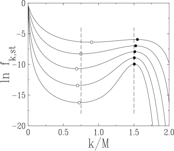
Figure 3: Logarithmic plot of the occupation probability $f_{k,{\rm st}}$ in the condensed phase ($b=4$, $\rho=4\rho_{c}=2$), against the ratio $k/M$. Top to bottom: $M=20$, 40, 80, 160, and 320. Full lines: $f_{k,{\rm st}}$ obtained by (5.4) and (5.5). Full (empty) symbols: maxima (minima) of occupation probability. Dashed vertical lines: asymptotic locations of the minima: $k/M=\Delta/(2M)=(\rho-\rho_{c})/2=3/4$, and of the maxima: $k/M=\Delta/M=\rho-\rho_{c}=3/2$.

We first analyse the behaviour of the occupation probability $f_{k,{\rm st}}$ in the condensed phase. Figure 3 shows a logarithmic plot of $f_{k,{\rm st}}$, computed using equations (5.4) and (5.5), against the ratio $k/M$, for $b=4$, $\rho=2$, and several values of $M$. This plot exhibits the following features.

• For $k\ll M$, the distribution $f_{k,{\rm st}}$ is approximately given by the power law (6.4) of an infinite critical system.

• The contribution of the condensate slowly builds up as a probability hump around $k=\Delta=M(\rho-\rho_{c})$, the mean number of excess particles.

• One observes a broad and shallow probability “dip” in the region located between the critical background and the condensate hump, i.e., in the region $k\gg 1$ and $\Delta-k\gg 1$.

The region of the dip is dominated by configurations where the excess particles are shared by two sites. Indeed, one has (see [19] for a proof)

$$f_{k,{\rm st}}\approx(b-1)\Gamma(b)\frac{\Delta^{b}}{k^{b}(\Delta-k)^{b}}\qquad(k\gg 1,\Delta-k\gg 1).$$ (9.1)

The observed locations of the maxima ($k\approx\Delta$) and minima ($k\approx\Delta/2$) of the occupation probability corroborate this picture, as explained in the caption of figure 3.

These observations lead to the following crude estimate for the characteristic time:

$$\tau\sim\frac{1}{f_{\rm min}},$$ (9.2)

since the minimum $f_{\rm min}$ of $f_{k,{\rm st}}$ corresponds to a barrier to cross, in the spirit of the Arrhenius law. The limiting scale of time is that required for the passage of this potential barrier. Eq. (9.1) implies that $f_{\rm min}$ is reached near the middle of the dip region $(k\approx N/2)$, and therefore (9.2) yields

$$\tau\sim\Delta^{b}.$$ (9.3)

We now present a more precise treatment. Assume that the condensate is on site number 1 at the initial observation time ($t=0$). The number $N_{1}(t)$ of particles on that site is initially very large, $N_{1}(0)\approx\Delta$, and therefore evolves slowly, until the condensate dissolves into the critical background. Thus

• We single out $N_{1}(t)$ as the collective co-ordinate of the system, that is the appropriate slow variable describing the dynamics of the condensate.

• We model the dynamics of $N_{1}(t)$ by (4.1), i.e., by a biased diffusive motion on the interval $k=0,\dots,N$. The left hopping rate is taken equal to the microscopic rate: $\mu_{k}=u_{k}$. The right hopping rate $\lambda_{k}$ is chosen such that, in the stationary state, the probability $f_{k,{\rm st}}$ of the effective model coincide with the occupation probability (5.5) of the original ZRP. The detailed balance condition (4.2) yields

  $$\lambda_{k}=\frac{\mu_{k+1}f_{k+1,{\rm st}}}{f_{k,{\rm st}}}=\frac{Z_{M-1,N-k-1}}{Z_{M-1,N-k}}=\bar{u}_{\rm st}(M-1,N-k),$$

  where the right side of the equation is the average rate coming from $M-1$ sites, containing $N-k$ particles (see (5.11)). The rate $\lambda_{k}$ is thus a function of $k$, $M$, and $N$. For $M=2$, this formula gives $\lambda_{k}=u_{N-k}$, as expected. In the fluid phase, in the thermodynamic limit, the rates $\lambda_{k}$ converge to $z_{0}$, defined in (5.8). Finally, for the condensed phase, in the dip region, we obtain

  $$\lambda_{k}\approx 1+\frac{b}{\Delta-k}\equiv u_{\Delta-k}.$$

This effective description reduces the full model to a Markovian model for one degree of freedom in an asymmetric potential. The two valleys of the potential are separated by a high (power-law) barrier. The left potential valley, corresponding to the critical background, has a weight $P_{\rm L}\approx 1$, whereas the right potential valley, corresponding to the hump of the condensate, has a weight $P_{\rm R}\approx 1/M\ll 1$ (see section 6.2).

In this framework the stationary dynamics of the condensate is characterised by a single diverging timescale. We choose to define this timescale, denoted by $\tau_{\scriptscriptstyle\rm Markov}$, to be the crossing time $T_{\rm L}$ from the right valley to the left one in the effective Markovian problem. The characteristic time is thus expressed by

$$\tau_{\scriptscriptstyle\rm Markov}\equiv T_{\rm L}=\sum_{\ell=1}^{N}\frac{1}{\mu_{\ell}f_{\ell,{\rm st}}}\sum_{m=\ell}^{N}f_{m,{\rm st}},$$ (9.4)

in terms of known quantities, the rates $\mu_{k}$ and the stationary probabilities $f_{k,{\rm st}}$. Its asymptotic growth is easily determined by noting that (9.4) is dominated by the behaviour of the probability $f_{k,{\rm st}}$ in the region of the dip. Hence, inserting the expression (9.1) into (9.4), and evaluating the sum as an integral, we obtain

$$\tau_{\scriptscriptstyle\rm Markov}\approx\frac{b\Gamma(b+1)}{(b-1)\Gamma(2b+2)}\,\frac{\Delta^{b+1}}{M}=\frac{b\Gamma(b+1)}{(b-1)\Gamma(2b+2)}\,(\rho-\rho_{c})^{b+1}M^{b}.$$ (9.5)

In order to compare the above theoretical predictions to the measured flipping time $\tau$, we compute the two-time stationary correlation function

$$C(t,0)=\langle N_{1}(t)N_{1}(0)\rangle-\rho^{2}.$$

This quantity decays exponentially with a relaxation constant which gives a natural measure of $\tau$. It is found that $\tau\sim\tau_{\scriptscriptstyle\rm Markov}\sim M^{b}$ in the MF and 1DAS geometries, and that $\tau\sim M\tau_{\scriptscriptstyle\rm Markov}\sim M^{b+1}$ in the 1DS geometry. For the latter case the occurence of one supplementary power in the system size has the same origin as for nonequilibrium dynamics.

9.4 Last remarks

Table 1 summarises the values of the dynamical exponents $z$ and $Z$, such that $\tau_{\rm non-st}\sim M^{z}$ and $\tau\sim M^{Z}$, where $\tau$ is the characteristic timescale for the stationary motion of the condensate.

Geometry	$z$	$Z$
MF, 1DAS	2	$b$
1DS	3	$b+1$

Table 1: Non-stationary and stationary dynamical exponents of the ZRP with static exponent $b>2$.

As recalled above, the non-stationary dynamical exponents are insensitive to the exponent $b$, and more generally to the statics, provided the system is in its condensed phase. This feature is easily understood in the context of the Markovian Ansatz proposed in the present work. Indeed the last stage of the formation of the condensate, i.e., the disappearance of the smaller of the last two precursors, implies no barrier crossing. In terms of the occupation of the condensate, it corresponds to the transition from $N_{1}$ to $\Delta$, where the initial occupation $N_{1}$ of the larger precursor was already larger than $\Delta/2$, corresponding to the top of the potential barrier. This explains why $\tau_{\rm non-st}$ is given by the diffusive timescale, both in the framework of the Markovian Ansatz and in the MF and 1DAS geometries.

10 Further references

Complementary aspects to the present notes can be found in [11, 38, 39, 40].

Appendix: Proof of eqs. (1.12) and (1.13)

We recall the fundamental equation (1.4)

$$p(W_{k,l}-W_{k,0})+q(W_{l,k}-W_{l,0})=$$

$$p\,\left(W_{k+1,l-1}\,\frac{p_{k+1}p_{l-1}}{p_{k}p_{l}}-W_{l,0}\right)+q\,\left(W_{l+1,k-1}\,\frac{p_{k-1}p_{l+1}}{p_{k}p_{l}}-W_{k,0}\right).$$ (A.1)

We first prove (1.12) for the symmetric case, $p=1/2$. Setting $x_{k}=W_{k,l}\,p_{k}p_{l}$, where $k+l=n$, (Appendix: Proof of eqs. (1.12) and (1.13)) can be rewritten as

$$x_{k}-x_{n-(k-1)}=x_{k+1}-x_{n-k}.$$

This expression is therefore a constant independent of $k$, which is equal to zero, as can be seen by taking $k=n$. We thus obtain

$$x_{k+1}=x_{n-k}$$

which is the detailed balance condition

$$p_{k}p_{l}\,W_{k,l}=p_{k-1}p_{l+1}\,W_{l+1,k-1}.$$ (A.2)

We now show that in the general case, $p\neq 1/2$, eq. (Appendix: Proof of eqs. (1.12) and (1.13)) yields two constraints on the rate: eq. (A.2) to be interpreted as the pairwise balance condition, and eq. (1.13)

$$W_{l,k}-W_{k,l}=W_{l,0}-W_{k,0}.$$ (A.3)

Set $a_{k}=p_{k}p_{l}\,W_{k,l}$. Eq. (Appendix: Proof of eqs. (1.12) and (1.13)) can be rewritten as

$$y_{k+1}-y_{k}=(p-q)(a_{n-k}-a_{k})$$ (A.4)

where

$$y_{k}=p\,x_{k}-q\,x_{n-(k-1)},\qquad y_{0}=0.$$ (A.5)

If

$$y_{k+1}=y_{n-k}$$ (A.6)

then it follows immediately that $x_{k+1}=x_{n-k}$, which is the condition for pairwise balance seen above. This relation itself plugged into (A.5), yields

$$x_{k+1}-x_{k}=a_{n-k}-a_{k}$$

which is (A.3). In order to prove (A.6) we set

$$A_{k}=a_{1}+\ldots+a_{k}$$

i.e. $a_{k}=A_{k}-A_{k-1}$. We thus have

$$y_{k}+(p-q)(A_{k-1}+A_{n-k})=y_{k+1}+(p-q)(A_{k}+A_{n-k-1})$$

which is equal to $(p-q)A_{n}$, hence

$$y_{k}=(p-q)(A_{n}-A_{n-k}-A_{k}+a_{k}).$$

Therefore $y_{k}-(p-q)a_{k}$ is symmetric in the change $k\to n-k$, and finally

$$y_{k}-(p-q)a_{k}=y_{n-k}-(p-q)a_{n-k}$$

which, using (A.4), yields (A.6).

References

References

- [1] Spitzer F 1970 Advances in Math. 5 246
- [2] Andjel E D 1982 Ann. Prob. 10 525
- [3] Schütz G M, Ramaswamy R and Barma M 1996 J. Phys. A 29 837
- [4] Ritort F 1995 Phys. Rev. Lett. 75 1190
- [5] For a review, see: Godrèche C and Luck J M 2002 J. Phys. Cond. Matt. 14 1601
- [6] Bialas P, Burda Z and Johnston D 1997 Nucl. Phys. B 493 505 Bialas P, Burda Z and Johnston D 1999 Nucl. Phys. B 542 413
- [7] Drouffe J M, Godrèche C and Camia F 1998 J. Phys. A 31 L19
- [8] Godrèche C and Luck J M 2001 Eur. Phys. J. B 23 473
- [9] Godrèche C 2003 J. Phys. A 36 6313
- [10] Cocozza-Thivent C 1985 Z. Wahr. 70 509
- [11] Evans M R and Hanney T 2005 J. Phys. A 38 R195
- [12] Godrèche C and Luck J M in preparation
- [13] Grosskinsky S and Spohn H 2003 Bull. Braz. Math. Soc. 34 489
- [14] Evans M R and Hanney T 2003 J. Phys. A 36 L44
- [15] Kolmogorov A N 1936 Math Ann. 112 115
- [16] Kelly F 1979 Reversibility and Stochastic Networks Wiley
- [17] Godrèche C, Levine E and Mukamel D 2005 J. Phys. A 38 L523
- [18] Godrèche C 2006 condmat/0603249
- [19] Godrèche C and Luck J M 2005 J. Phys. A 38 7215
- [20] Ehrenfest P and T 1907 Phys. Zeit. 8 311
- [21] Kac M 1947 Amer. Math. Monthly 54 369 Kac M 1959 Probability and Related Topics in Physical Sciences Lectures in Applied Mathematics vol 1 A (American Mathematical Society)
- [22] Evans M R 2000 Braz. J. Phys. 30 42
- [23] O’Loan O J, Evans M R and Cates M E 1998 Phys. Rev. E 58 1404
- [24] Majumdar S N, Evans M R and Zia R K P 2005 Phys. Rev. Lett. 94 180601 Evans M R, Majumdar S N and Zia R K P 2005 cond-mat/0510512
- [25] Grosskinsky S, Schütz G M and Spohn H 2003 J. Stat. Phys. 113 389
- [26] Kafri Y, Levine E, Mukamel D, Schütz G M and Török J 2002 Phys. Rev. Lett. 89 035702
- [27] Kaupuzs J, Mahnke R and Harris R J 2005 Phys. Rev. E 72 056125
- [28] Feller W 1966 An Introduction to Probability Theory and its Applications (New-York: Wiley) vol 1
- [29] Cordery R, Sarker S and Tobochnik J 1981 Phys. Rev. B 24 5402 Cornell S J, Kaski K and Stinchcombe R B 1991 Phys. Rev. B 44 12263 Cornell S J and Bray A J 1996 Phys. Rev. E 54 1153 Ben-Naim E and Krapivsky P L 1998 J. Stat. Phys. 93 583 Godrèche C and Luck J M 2003 J. Phys. A 36 9973
- [30] Bray A J 1994 Adv. Phys. 43 357
- [31] Godrèche C and Luck J M 2002 J. Phys. Cond. Matt. 14 1589
- [32] Cugliandolo L and Kurchan J 1994 J. Phys. A 27 5749
- [33] Godrèche C and Luck J M 2000 J. Phys. A 33 9141
- [34] Godrèche C and Luck J M 2000 J. Phys. A 33 1151
- [35] Janssen H K, Schaub B and Schmittmann B 1989 Z. Phys. B 73 539
- [36] Huse D A 1989 Phys. Rev. B 40 304
- [37] Cugliandolo L F, Kurchan J and Peliti L 1997 Phys. Rev. E 55 3898 Barrat A 1998 Phys. Rev. E 57 3629 Berthier L, Barrat J L and Kurchan J 1999 Eur. Phys. J. B 11 635
- [38] Kipnis C and Landim C 1999 Scaling limits of interacting particle systems Springer
- [39] Bertini L, De Sole A, Gabrielli D, Jona-Lasinio G and Landim C 2002 J. Stat. Phys. 107 635
- [40] Harris R J, Rakos A and Schütz G 2005 J. Stat. Mech. P08003