Temporal Oscillation of Conductances in Quantum Hall Effect of Bloch Electrons

Abstract

We study a nonadiabatic effect on the conductances in the quantum Hall effect of two-dimensional electrons with a periodic potential. We found that the Hall and longitudinal conductances oscillate in time with very large frequencies due to quantum fluctuation.

Two years after the discovery of the quantum Hall effect [1, 2], Thouless, Kohmoto, Nightingale and den Nijs (TKNN) [3, 4] theoretically studied the quantum Hall effect in two-dimensional electrons with a periodic potential. They expressed the Hall conductance as an integer multiplied by $e^{2}/h$. The integer is a topological invariant called the Chern number. Such a system has been experimentally realized as a superlattice structure in a semi-conductor heterojunction. [5, 6, 7]

We can treat the electric field as a time-dependent vector potential. Then adiabatic approximation gives the same expression of the Hall conductance as in the TKNN theory.[8, 9] In this Letter, we consider the conductances of the same system taking a nonadiabatic effect into account. We determine the quantum fluctuation of the Hall conductance $\sigma_{xy}$ and the longitudinal conductance $\sigma_{yy}$; i.e., $\sigma_{xy}$ and $\sigma_{yy}$ oscillate in time with very large frequencies.

We consider the nonadiabatic effect on the conductances with the help of the Greenwood linear-response theory[10] and study a correction to the adiabatic approximation. Wagner studied the failure of the Kubo formula due to a nonadiabatic effect on the dc current in a finite system. [11, 12] Grimaldi et al. explained the high-$T_{\rm c}$ superconductivity of fullerene compounds by taking nonadiabatic effects into account.[13]

This Letter is organized as follows. We first calculate the conductances beyond the adiabatic approximation and obtain correction terms to $\sigma_{xy}$ and $\sigma_{yy}$ of the TKNN theory. We then evaluate the oscillations in these correction terms numerically.

We consider noninteracting electrons in a periodic potential in the $x$-$y$ plane. A magnetic field is applied in the $z$ direction, and an electric field is applied in the $y$ direction. We treat the electric field as a vector potential. Using the Landau gauge, we express the Hamiltonian of the system as

$$\mathcal{H}(t)=\frac{1}{2m_{\rm e}}\left(\mbox{\boldmath$p$}+e\mbox{\boldmath$A$}(t)\right)^{2}+U(\mbox{\boldmath$x$}),$$ (1)

where

$$\mbox{\boldmath$A$}(t) = \left(Bx-E_{y}t\right)\mbox{\boldmath$e$}_{y},$$

$$U(\mbox{\boldmath$x$}) = U_{x}\cos\left(\frac{2\pi x}{a}\right)+U_{y}\cos\left(\frac{2\pi y}{b}\right).$$ (2)

We consider the flux per unit cell of $U(\mbox{\boldmath$x$})$ to be the rational number $p/q$ in the unit of the flux quantum, which produces $p$ subbands. We label each subband by $m\;(1\leq m\leq p)$ hereafter. Then we obtain the generalized crystal momentum $\hbar\mbox{\boldmath$k$}$ defined in the magnetic Brillouin zone.[14] $0\leq k_{x}<2\pi/qa$ and $0\leq k_{y}<2\pi/b$.

We define $\mathcal{H}_{\mbox{\boldmath$k$}}(t)$ as

$$\mathcal{H}_{\mbox{\boldmath$k$}}(t)\equiv{\rm e}^{-{\rm i}\mbox{\boldmath$k$}\cdot\mbox{\boldmath$x$}}\mathcal{H}(t){\rm e}^{{\rm i}\mbox{\boldmath$k$}\cdot\mbox{\boldmath$x$}}.$$ (3)

The instantaneous Hamiltonian $\mathcal{H}_{\mbox{\boldmath$k$}}(t)$ is diagonalized as

$$\mathcal{H}_{\mbox{\boldmath$k$}}(t)\left|u_{m\mbox{\boldmath$k$}}(\mbox{\boldmath$x$},t)\right\rangle=\epsilon_{m\mbox{\boldmath$k$}}(t)\left|u_{m\mbox{\boldmath$k$}}(\mbox{\boldmath$x$},t)\right\rangle.$$ (4)

Since $\mathcal{H}_{\mbox{\boldmath$k$}}(t)=\mathcal{H}_{k_{x},k_{y}-eE_{y}t/\hbar}(0)$, we obtain for $m\neq n$

$$\epsilon_{m\mbox{\boldmath$k$}}(t) = \epsilon_{m\mbox{\boldmath$k$}}(0)+O(E_{y}),$$

$$\left\langle u_{m\mbox{\boldmath$k$}}(\mbox{\boldmath$x$},t)|\dot{u}_{n\mbox{\boldmath$k$}}(\mbox{\boldmath$x$},t)\right\rangle =$$ (5)

$$\frac{eE_{y}}{\hbar}\left\langle\frac{\partial u_{m\mbox{\boldmath$k$}}(\mbox{\boldmath$x$},0)}{\partial k_{y}}\Biggm{|}u_{n\mbox{\boldmath$k$}}(\mbox{\boldmath$x$},0)\right\rangle+O\left(E_{y}^{2}\right),$$

where the dot indicates the time derivative. We note that, by fixing the arbitrary phase in each time, we can always achieve $\left\langle u_{m\mbox{\boldmath$k$}}(\mbox{\boldmath$x$},t)|\dot{u}_{m\mbox{\boldmath$k$}}(\mbox{\boldmath$x$},t)\right\rangle=0.$

The time evolution of the density operator is given by the von Neumann equation

$$\frac{{\rm d}}{{\rm d}t}\rho(t)=\frac{1}{{\rm i}\hbar}[\mathcal{H}(t),\rho(t)].$$ (6)

Following the Greenwood linear-response theory,[10] we expand the density operator with respect to the electric field and take the zeroth- and first-order terms into account

$$\rho(t)=\rho^{(0)}+E_{y}\rho^{(1)}(t).$$ (7)

Thus, the matrix elements

$$\rho_{mn\mbox{\boldmath$k$}}\equiv\left\langle u_{m\mbox{\boldmath$k$}}(\mbox{\boldmath$x$},t)\right|{\rm e}^{-{\rm i}\mbox{\boldmath$k$}\cdot\mbox{\boldmath$x$}}\rho(t){\rm e}^{{\rm i}\mbox{\boldmath$k$}\cdot\mbox{\boldmath$x$}}\left|u_{n\mbox{\boldmath$k$}}(\mbox{\boldmath$x$},t)\right\rangle$$ (8)

are approximated using

$$\rho_{mn\mbox{\boldmath$k$}} = \rho_{mn\mbox{\boldmath$k$}}^{(0)}+E_{y}\rho_{mn\mbox{\boldmath$k$}}^{(1)}$$ (9)

$$= f_{m}\delta_{mn}+E_{y}\rho_{mn\mbox{\boldmath$k$}}^{(1)},$$

where $f_{m}\;(=f(\epsilon_{m\mbox{\boldmath$k$}}))$ is the Fermi distribution. Hereafter, we let $\epsilon_{m\mbox{\boldmath$k$}}$ denote $\epsilon_{m\mbox{\boldmath$k$}}(0)$ and $\left|u_{m\mbox{\boldmath$k$}}\right\rangle$ denote $\left|u_{m\mbox{\boldmath$k$}}(\mbox{\boldmath$x$},0)\right\rangle$.

The time evolution of the off-diagonal elements ($m\neq n$) is given by

$$\frac{{\rm d}}{{\rm d}t}\rho_{mn\mbox{\boldmath$k$}}^{(1)}=\frac{1}{{\rm i}\hbar}(\epsilon_{m\mbox{\boldmath$k$}}-\epsilon_{n\mbox{\boldmath$k$}})\rho_{mn\mbox{\boldmath$k$}}^{(1)}+\frac{e}{\hbar}(f_{m}-f_{n})\left\langle\frac{\partial u_{m\mbox{\boldmath$k$}}}{\partial k_{y}}\Biggm{|}u_{n\mbox{\boldmath$k$}}\right\rangle.$$ (10)

Therefore, we obtain the matrix elements of the density operator as

$$\rho_{mn\mbox{\boldmath$k$}}^{(1)} = -{\rm i}e\left\langle\frac{\partial u_{m\mbox{\boldmath$k$}}}{\partial k_{y}}\Biggm{|}u_{n\mbox{\boldmath$k$}}\right\rangle\frac{f_{m}-f_{n}}{\epsilon_{m\mbox{\boldmath$k$}}-\epsilon_{n\mbox{\boldmath$k$}}}\left[1-{\rm e}^{-{\rm i}(\epsilon_{m\mbox{\boldmath$k$}}-\epsilon_{n\mbox{\boldmath$k$}})t/\hbar}\right]\quad(m\neq n),$$ (11)

$$\rho_{mm\mbox{\boldmath$k$}}^{(1)} =$$ const. (12)

Let us calculate the current $J_{\alpha}\;(\alpha=x,y)$ using

$$J_{\alpha} \equiv {\rm Re}\left[\langle J_{\alpha}(E_{y})\rangle-\langle J_{\alpha}(0)\rangle\right],$$ (13)

$$\langle J_{\alpha}(E_{y})\rangle = {\rm Tr}\left(\rho(t)\frac{\partial\mathcal{H}(t)}{\partial A_{\alpha}(t)}\right)$$ (14)

$$= \frac{e}{\hbar}{\rm Tr}\left(\rho_{\mbox{\boldmath$k$}}(t)\frac{\partial\mathcal{H}_{\mbox{\boldmath$k$}}(t)}{\partial k_{\alpha}}\right).$$

By plugging eqs. (11) and (12) into eq. (14), we obtain

$$J_{\alpha}=\frac{e^{2}}{\hbar}E_{y}{\rm Re}\int_{\rm MBZ}\frac{{\rm d}^{2}\mbox{\boldmath$k$}}{(2\pi)^{2}}\sum_{m\neq n}{\rm i}(f_{m}-f_{n})\left\langle\frac{\partial u_{m\mbox{\boldmath$k$}}}{\partial k_{y}}\Biggm{|}u_{n\mbox{\boldmath$k$}}\right\rangle\left\langle u_{n\mbox{\boldmath$k$}}\Biggm{|}\frac{\partial u_{m\mbox{\boldmath$k$}}}{\partial k_{\alpha}}\right\rangle\left[1-{\rm e}^{-{\rm i}(\epsilon_{m\mbox{\boldmath$k$}}-\epsilon_{n\mbox{\boldmath$k$}})t/\hbar}\right],$$ (15)

where MBZ denotes the magnetic Brillouin zone. After some tedious but straightforward calculation, we obtain the conductances $\sigma_{xy}$ and $\sigma_{yy}$ in the forms

$$\sigma_{xy} \equiv \frac{J_{x}}{E_{y}}$$

$$= \frac{e^{2}}{2\pi\hbar}N_{\rm Ch}+\frac{e^{2}}{\hbar}\int_{\rm MBZ}\frac{{\rm d}^{2}\mbox{\boldmath$k$}}{(2\pi)^{2}}\sum_{m\neq n}(f_{m}-f_{n})r_{mn}(\mbox{\boldmath$k$})\sin{\left[(\epsilon_{m\mbox{\boldmath$k$}}-\epsilon_{n\mbox{\boldmath$k$}})t/\hbar-\theta_{mn}(\mbox{\boldmath$k$})\right]},$$

$$\sigma_{yy} \equiv \frac{J_{y}}{E_{y}}$$

$$= \frac{e^{2}}{\hbar}\int_{\rm MBZ}\frac{{\rm d}^{2}\mbox{\boldmath$k$}}{(2\pi)^{2}}\sum_{m\neq n}\left|\left\langle\frac{\partial u_{m\mbox{\boldmath$k$}}}{\partial k_{y}}\Biggm{|}u_{n\mbox{\boldmath$k$}}\right\rangle\right|^{2}\left(f_{m}-f_{n}\right)\sin{(\epsilon_{m\mbox{\boldmath$k$}}-\epsilon_{n\mbox{\boldmath$k$}})t/\hbar},$$

where $r_{mn}(\mbox{\boldmath$k$})$ and $\theta_{mn}(\mbox{\boldmath$k$})$ are the real numbers that satisfy

$$r_{mn}(\mbox{\boldmath$k$}){\rm e}^{{\rm i}\theta_{mn}(\mbox{\boldmath$k$})}\equiv\left\langle\frac{\partial u_{m\mbox{\boldmath$k$}}}{\partial k_{y}}\Biggm{|}u_{n\mbox{\boldmath$k$}}\right\rangle\left\langle u_{n\mbox{\boldmath$k$}}\Biggm{|}\frac{\partial u_{m\mbox{\boldmath$k$}}}{\partial k_{x}}\right\rangle.$$ (17)

Here, $N_{\rm Ch}$ is the Chern number with a finite-temperature correction

$$N_{\rm Ch}\equiv\sum_{m}f_{m}\int_{\rm MBZ}\frac{{\rm d}^{2}\mbox{\boldmath$k$}}{\pi}{\rm Im}\left[\left\langle\frac{\partial u_{m\mbox{\boldmath$k$}}}{\partial k_{y}}\Biggm{|}\frac{\partial u_{m\mbox{\boldmath$k$}}}{\partial k_{x}}\right\rangle\right].$$ (18)

We note that if we ignore the time dependence of $\rho_{mn\mbox{\boldmath$k$}}^{(1)}$ in eq. (10), we obtain $\sigma_{xy}=(e^{2}/2\pi\hbar)N_{\rm Ch}$ and $\sigma_{yy}=0$, which are consistent with the TKNN theory.

The above-mentioned equations imply that we obtain sinusoidally oscillating terms in addition to the Chern-number term in the Hall conductance $\sigma_{xy}$ due to quantum fluctuation. The longitudinal conductance $\sigma_{yy}$ also oscillates with zero mean. The oscillation period is determined by the energy-gap size.

Equation (LABEL:fullsigma) is also a gauge invariant. We observe this by treating the electric field as the scalar potential $A_{0}(t)=-eE_{y}y\exp[-{\rm i}\omega t]$ instead of the vector potential. The first-order time-dependent perturbation theory gives eqs. (15) and (LABEL:fullsigma) in the limit of $\omega\to 0$.

To demonstrate the oscillation numerically, we assume that the state lies in the lowest Landau level. Moreover, we assume that the flux $\Phi\;(=abB)$ is given by the unit flux $\Phi_{0}\;(=2\pi\hbar/e)$ multiplied by the rational number $p/q$ as

$$\frac{\Phi}{\Phi_{0}}=\frac{abeB}{2\pi\hbar}=\frac{p}{q},$$ (19)

where $p$ and $q$ are coprime. Due to the periodic potential $U(x,y)$, each Landau level splits into $p$ subbands with a $q$-fold degeneracy in each subband.

In the weak-potential limit $|U(\mbox{\boldmath$x$})|\ll\hbar eB/m_{\rm e}$, the perturbation theory gives the instantaneous eigenfunction $\left|u_{m\mbox{\boldmath$k$}}(\mbox{\boldmath$x$})\right\rangle$ as[3]

$$\left|u_{m\mbox{\boldmath$k$}}(\mbox{\boldmath$x$})\right\rangle = \frac{1}{\sqrt{\mathcal{N}}}\sum_{\nu=1}^{p}d_{m}^{\nu}(\mbox{\boldmath$k$})\sum_{\ell=-\infty}^{\infty}\exp\left[-\left(\frac{eB}{2\hbar}\right)\left(x+\frac{\hbar k_{y}}{eB}-\ell qa-\frac{\nu qa}{p}\right)^{2}\right]$$ (20)

$$\times \exp\left[-{\rm i}k_{x}\left(x-\ell qa-\frac{\nu qa}{p}\right)\right]{\rm e}^{-2\pi{\rm i}y\frac{\ell p+\nu}{b}},$$

where $\mathcal{N}$ is the normalization factor. Here, the coefficients $\{d_{m}^{\nu}\}$ and first-order energy shift $\epsilon^{(1)}_{m\mbox{\boldmath$k$}}$ are determined by the following secular equation.

$$\beta d_{m}^{\nu-1}(\mbox{\boldmath$k$})+\alpha_{\nu}d_{m}^{\nu}(\mbox{\boldmath$k$})+\beta^{*}d_{m}^{\nu+1}(\mbox{\boldmath$k$})=\epsilon^{(1)}_{m\mbox{\boldmath$k$}}d_{m}^{\nu}(\mbox{\boldmath$k$}).$$ (21)

Here,

$$\alpha_{\nu} = U_{x}{\rm e}^{-\pi qb/2pa}\cos{(-qbk_{y}/p+2\pi\nu q/p)},$$

$$\beta = \frac{U_{y}}{2}{\rm e}^{-\pi qa/2pb}{\rm e}^{-{\rm i}qak_{x}/p}.$$ (22)

Note that the unperturbed energy $\epsilon^{(0)}_{m\mbox{\boldmath$k$}}$ is independent of $m$ and $k$; i.e., $\epsilon_{m\mbox{\boldmath$k$}}-\epsilon_{n\mbox{\boldmath$k$}}=\epsilon^{(1)}_{m\mbox{\boldmath$k$}}-\epsilon^{(1)}_{n\mbox{\boldmath$k$}}$. After straightforward calculation, we obtain

$$\left\langle\frac{\partial u_{m\mbox{\boldmath$k$}}}{\partial k_{x}}\Biggm{|}\frac{\partial u_{m\mbox{\boldmath$k$}}}{\partial k_{y}}\right\rangle = \sum_{\nu=1}^{p}\left(\frac{{\rm d}d_{m}^{\nu}}{{\rm d}k_{x}}\right)^{*}\frac{{\rm d}d_{m}^{\nu}}{{\rm d}k_{y}}-{\rm i}\frac{\hbar}{eB},$$ (23)

$$\left\langle u_{n\mbox{\boldmath$k$}}\Biggm{|}\frac{\partial u_{m\mbox{\boldmath$k$}}}{\partial k_{x}}\right\rangle = \sum_{\nu=1}^{p}\left(d_{n}^{\nu}\right)^{*}\frac{{\rm d}d_{m}^{\nu}}{{\rm d}k_{x}},$$ (24)

$$\left\langle u_{n\mbox{\boldmath$k$}}\Biggm{|}\frac{\partial u_{m\mbox{\boldmath$k$}}}{\partial k_{y}}\right\rangle = \sum_{\nu=1}^{p}\left(d_{n}^{\nu}\right)^{*}\frac{{\rm d}d_{m}^{\nu}}{{\rm d}k_{y}}.$$ (25)

Thus, we can calculate the conductances $\sigma_{xy}$ and $\sigma_{yy}$ in eq. (LABEL:fullsigma) using the eigenvalues and eigenvectors in eq. (21).

As typical values, we use $a=100{\rm nm}$, $b=130{\rm nm}$, and $U_{x}=U_{y}=0.1{\rm meV}$. We assume $p/q=65/2$, implying $B=10.4{\rm T}$. With this flux ratio, the lowest Landau level splits into 65 subbands. We note that the $p$ subbands in the lowest Landau level range from $0.240{\rm meV}$ to $0.948{\rm meV}$. The center of the next Landau level is located at $1.78{\rm meV}$. In the numerical calculation, we obtain the derivatives of $d_{m}^{\nu}(\mbox{\boldmath$k$})$ by the finite-difference method. We consider the slices $\Delta k_{x}$ and $\Delta k_{y}$ to be $2\pi/100qa$ and $2\pi/100b$, respectively. The Chern number term is obtained by Fukui, Hatsugai and Suzuki’s method[15].

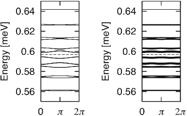
First, we make the Fermi energy $\epsilon_{\rm F}$ lie between the 33rd and 34th levels, as shown in Fig. 1. The fluctuations of $\sigma_{xy}$ and $\sigma_{yy}$ in Fig. 2 consist of the oscillations corresponding to the energy gaps between levels higher than $\epsilon_{\rm F}$ and levels lower than $\epsilon_{\rm F}$. Figure 2 shows that the time resolution required to detect the quantum fluctuation is about $10{\rm ps}$. 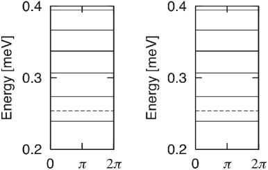Secondly, we make $\epsilon_{\rm F}$ lie between the second and third levels, as shown in Fig. 3. Then we obtain almost periodic oscillations of $\sigma_{xy}$ and $\sigma_{yy}$ (Fig. 4) in contrast to the seemingly random oscillation in the former case. This is because the energy gaps are almost constant in the latter case.

Figure 1: The energy levels around the center of the $p\;(=65)$ subbands are shown as functions of (a) $qak_{x}$ and (b) $bk_{y}$. The flux ratio $p/q=65/2$ corresponds to $B=10.4{\rm T}$. We use $U_{x}=U_{y}=0.1{\rm meV}$, $a=100{\rm nm}$, and $b=130{\rm nm}$. The Fermi energy (the dashed line) lies between the 33rd and 34th levels.

Figure 2: Conductances corresponding to the situation in Fig. 1. In the upper panel, the solid line shows $\sigma_{xy}$ as a function of time, and the dashed line shows the Chern number term $\sigma_{\rm Ch}=(e^{2}/2\pi\hbar)N_{\rm Ch}$. In this case, $N_{\rm Ch}=1$. The lower panel shows $\sigma_{yy}$ as a function of time.

Figure 3: The energy levels in the lowest part of the $p\;(=65)$ subbands are shown as functions of (a) $qak_{x}$ and (b) $bk_{y}$. The flux ratio $p/q=65/2$ corresponds to $B=10.4{\rm T}$. We use $U_{x}=U_{y}=0.1{\rm meV}$, $a=100{\rm nm}$, and $b=130{\rm nm}$. The Fermi energy (the dashed line) lies between the second and third levels. In each panel, the lowest solid line below the dashed line expresses the degenerate first and second levels.

Figure 4: Conductances corresponding to the situation in Fig. 3. In the upper panel, the solid line shows $\sigma_{xy}$ as a function of time, and the dashed line shows the Chern number term $\sigma_{\rm Ch}=(e^{2}/2\pi\hbar)N_{\rm Ch}$. In this case, $N_{\rm Ch}=0$. The lower panel shows $\sigma_{yy}$ as a function of time.

To summarize, we studied a nonadiabatic effect on the conductances in the TKNN theory. We found that both $\sigma_{xy}$ and $\sigma_{yy}$ oscillate due to quantum fluctuation. The oscillation period is of the order of $100{\rm ps}$ to $1{\rm ns}$. It is a challenging but interesting issue to detect these oscillations experimentally.

Although we studied the time dependence of currents at a constant electric field, by similar calculation, we observe that constant currents in reverse produce a time-dependent electric field. In this case, the oscillation period is also determined by the energy-gap size.