A General Theorem Relating the Bulk Topological Number to Edge States
in Two-dimensional Insulators

Abstract

We prove a general theorem on the relation between the bulk topological quantum number and the edge states in two dimensional insulators. It is shown that whenever there is a topological order in bulk, characterized by a non-vanishing Chern number, even if it is defined for a non-conserved quantity such as spin in the case of the spin Hall effect, one can always infer the existence of gapless edge states under certain twisted boundary conditions that allow tunneling between edges. This relation is robust against disorder and interactions, and it provides a unified topological classification of both the quantum (charge) Hall effect and the quantum spin Hall effect. In addition, it reconciles the apparent conflict between the stability of bulk topological order and the instability of gapless edge states in systems with open boundaries (as known happening in the spin Hall case). The consequences of time reversal invariance for bulk topological order and edge state dynamics are further studied in the present framework.

I Introduction

Since the discovery of the quantized Hall effect two decades agovon Klitzing et al. (1980), topological quantum number has been well accepted as an important characterization of quantum many-body systems. The quantized Hall conductance in the integer quantum Hall effect is first identified, for non-interacting electrons on a lattice, as a first Chern number over the magnetic Brillouin zone by Thouless et al.Thouless et al. (1982), which is also known as the TKNN number. However, this characterization does not apply to systems with impurity and/or interactions, since the Brillouin zone is not defined for these systems. The study on momentum space topologyVolovik (2003) can be viewed as the developments along this direction. It indeed goes beyond the non-interacting fermion system, by considering the poles of the single particle Green function, but it pre-requires the Fermi liquid property of the system. To define a topological characterization for general many-body systems, Niu et al.Niu et al. (1985) introduced the technique of twisted boundary conditions, and showed that the first Chern number can be generally defined over the parameter space of twisted phases for any two dimensional insulator.

One of the important observable consequences of the bulk topological invariance in quantum Hall systems is the presence of gapless (chiral) edge states on the boundary of the system. Just like the existence of gapless Goldstone modes is a characteristic of the spontaneous breaking of a continuous symmetry, the existence of gapless edge excitations can be considered as a manifestation of bulk “topological order”, defined through the topological quantum numbers. According to Laughlin and Halperin’s gauge argumentLaughlin (1981); Halperin (1982), $n$ branches of gapless edge states must exist for a system with Hall conductance $\sigma_{H}=ne^{2}/h$, since there must be $n$ electrons transferred from one edge to the other when a unit flux $2\pi$ is adiabatically threaded through a cylindrical system. The physical intuition of this argument inspired later HatsugaiHatsugai (1993a, b) to demonstrate an explicit and rigorous relation between the bulk TKNN number and the dynamics of edge states. He has succeeded in finding a topological characterization of edge states and then proved that the edge topological number is equal to the bulk TKNN number. However, this relation cannot be generalized to more general many-body systems, where the TKNN number has to be replaced by a more general Chern number as defined in Ref.Niu et al. (1985). Therefore, it is important to establish a general theorem, similar to the “Goldstone theorem” in the case spontaneous symmetry breaking, that bridges the bulk topological quantum number generally defined by the twisted boundary condition, and edge properties for a generic many-body system. To provide such a theorem is the main goal of the present paper.

This problem is not merely of academic interest, in view of the recent proposals of the intrinsic spin Hall effectMurakami et al. (2003); Sinova et al. (2004); Murakami et al. (2004); Kane and Mele (2005a) and the quantum spin Hall effectBernevig and Zhang (2006); Qi et al. ; Sheng et al. (2005). Two distinctly new issues arise in the topological characterization of the quantized spin Hall effect, compared to that of the quantized charge Hall effect, calling for a clearer understanding of the general relation between bulk topology and edge dynamics. Firstly, spin is in general not conserved due to spin-orbit coupling and, therefore, the Laughlin-Halperin gauge argument does not apply straightforwardly. However, by generalizing the twisted boundary conditions in Ref.Niu et al. (1985) to the spin channel, a Chern number can still be definedHatsugai (2005); Hatsugai et al. ; Sheng et al. . Thus the physical meaning of such bulk Chern number and its relation to the edge states in the quantized spin Hall case becomes less clear compared with the quantum Hall case. Secondly, the spin Hall systems of present interest respect time-reversal invariance, which leads to additional constraints on the possible Hamiltonians and on the edge dynamics. In Ref.Kane and Mele (2005b), Kane and Mele proposed a “$Z_{2}$ topological order” for T-invariant systems, in which the T-invariant systems are classified according to whether there are an even or odd number of Kramers pairs of edge states on each edge. Such a $Z_{2}$ characterization is protected by Kramers degeneracy and seems to be consistent with recent numerical resultsSheng et al. (2005, ). However, it remains unclear whether the $Z_{2}$ characterization can be generalized to many-body systems with impurities and/or interactions. Careful study on edge dynamicsWu et al. (2006); Xu and Moore (2006) shows that the edge states can become gapful with sizable strength of interactions, even for the case of an odd number of Kramers pairs. This suggests that the $Z_{2}$ classification may not be a topological order protected by the bulk gap alone, but depends on more subtle behavior of the system.

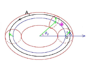
To clarify these issues, in this paper we propose a new framework to relate the bulk topological number to edge dynamics, by introducing generalized twisted boundary conditions. In the usual definition of twisted boundary conditions, the system is defined on a torus (namely a rectangle with side length L with the opposite boundaries in $x$- and $y$-directions identified, respectively); a particle gains an extra phase $e^{i\theta_{x}}$ (or $e^{i\theta_{y}}$) whenever it goes across the boundary in $x$ (or $y$-) direction. (The phases ($\theta_{x},\theta_{y}$) may be associated with the internal degrees of freedom in the case of the spin Hall effect.) Assuming that the many-body ground state of the system is separated from the excited states by a finite gap for all values of the twisted phases ($\theta_{x},\theta_{y}$), the first Chern number is then defined by the total flux of the Berry-phase gauge field associated with the ground state over the $(\theta_{x},\theta_{y})$-space, whose topology is a torus. To establish a bulk-edge connection, one may relate the toroidal system to a cylindrical system with open boundaries in the way as suggested in Ref. Wu (1990; pp. 461-491). The simplest thought is of course to cut the torus in real space along a circle, say located at $x=L$, resulting in a cylinder with two open boundaries at $x=0$ and $x=L$. Then a particle can no longer go across the boundary at $x=0$ or $x=L$. Conversely, one may view the toroidal system as obtained by gluing together the two edges of a cylindrical system. In quantum theory the gluing can be implemented by allowing a tunable tunnelling between the two edgesWu (1990; pp. 461-491). This leads to the idea of changing the twisted phase $e^{i\theta_{x}}$ of the toroidal system into a complex number $re^{i\theta_{x}}$, with $0\leq r\leq 1$. Namely we will allow the hopping amplitude of a particle across the $x$-boundary to be reduced by a factor $r$. When $r=0$, no particle can go across the $x$-boundary, and the spatial geometry of the system becomes a cylinder. With this generalized twisted boundary condition, the parameter space is now enlarged to three variables $(r,\theta_{x},\theta_{y})$. Since at $r=0$, different values of $\theta_{x}$ do not make any difference, the geometry of the parameter space is actually $D^{2}\times U(1)$, with $(r,\theta_{x})$ the polar coordinates of the disk $D^{2}$. In other words, the topology of the parameter 3-space is now that of a solid torus, the interior of a torus embedded in three dimensions: The toroidal surface at $r=1$ represents the original toroidal system, while the central loop at $r=0$ represents the associated cylindrical system. In this way, the solid torus implements a continuous interpolation between the toroidal and cylindrical systems. A schematic picture of the parameter space is shown in Fig. 1. In this framework, the bulk Chern number corresponds to the total magnetic flux through the toroidal surface at $r=1$, so inside the solid torus there must be magnetic monopole sources, i.e. singularities where degeneracy occurs due to the emergence of gapless edge states and breaks the adiabatic evolution and makes the Berry phase ill-defined. Consequently, the relation between bulk topology and edge dynamics is simply dictated by the (magnetic) Gauss theorem for the solid $(r,\theta_{x},\theta_{y})$ torus.

Figure 1: Schematic picture of the parameter space torus and the definition of coordinates $(r,\theta_{x},\theta_{y})$. A monopole singularity is drawn in the solid torus.

Once such a novel connection is established, more complete understanding on the quantum Hall (QH) and quantum spin Hall (QSH) systems can be achieved. It will be demonstrated that whenever the bulk topology is nontrivial, there must be gapless edge states in some twisted-boundary system with $(r,\theta_{x})(r<1)$, but the gaplessness of edge states does not have to occur in the open-boundary system with $r=0$. Only when the corresponding physical quantity in the twisted boundary conditions (charge for QHE and spin for QSHE) is conserved, can the gapless edge states be sure to happen in the open-boundary system. The “shift” of gapless edge states to generalized twisted boundary conditions provides a natural rationale to account for the gap opening in the edge channels in the spin Hall systemsXu and Moore (2006); Wu et al. (2006). Upon considering the time reversal invariance, some constraints on the winding number distribution is obtained and the $Z_{2}$ classification is shown to be related to the behavior of low energy excitations under time reversal, not merely to the bulk topology.

The rest of the paper is organized as follows: The proof of the general theorem on the relation between bulk topology and edge dynamics is given in Sec. II. Several examples are given in Sec. III, including the QHE and QSHE cases. The role of time reversal invariance is discussed and the $Z_{2}$ classification is analyzed in Sec. IV. Finally, Sec. V is devoted to summary and discussions.

II General Relation between Bulk Topology and Edge States

II.1 Generalized twisted boundary conditions and the bulk Chern number

There are two equivalent ways to define the twisted boundary conditions for a toroidal system. One is to impose constraints on the many body wave function of the form $\Phi({\bf r_{1}},{\bf r_{2}},..)=e^{i\theta}\Phi({\bf r_{1}}+L{\bf\hat{x}},\bf{r_{2}},..)$. The other is to add parameters into the Hamiltonian. Since we would like to study the Berry phase gauge field under adiabatic evolution, it is more convenient to choose the latter. For convenience, here we consider the many-body system on a lattice, with a Hamiltonian of the form

$$H_{0} = -\sum_{\left\langle ij\right\rangle}t_{ij,\alpha\beta}c_{i\alpha}^{\dagger}c_{j\beta}+H_{\rm int},$$ (1)

in which $c_{i\alpha}$ is the annihilation operator of boson or fermion at the site $i$, with $\alpha=1,\cdots,s$ labelling internal degrees of freedom. The first term is the nearest neighbor hopping term. The second term $H_{\rm int}$ may contain all possible disorder or interaction terms that conserve the local particle number: $\left[H_{\rm int},n_{i}\right]=0,\forall i$. The sites $i$ are defined on a 2-d lattice with size $L$ with periodic boundary conditions or, in other words, a lattice on a 2-torus $T^{2}$. Such a Hamiltonian (1) describes a wide class of interacting many-particle systems with nearest neighbor hoppings. Our treatment below can be generalized to more complex Hamiltonians as discussed later.

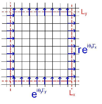
We introduce on $T^{2}$ two boundary lines $L_{x},L_{y}$ in the $x$ and $y$ direction, respectively, as shown in Fig. 2. The twisted Hamiltonian is defined by changing the hopping matrix elements across the boundary lines $L_{x},L_{y}$ only in the following way:

$$t_{ij}\rightarrow\left\{\begin{array}[]{c c}t_{ij}r{e^{i\Gamma_{x}\theta_{x}}},&\left\langle ij\right\rangle\text{ across }L_{x}\\ t_{ij}{e^{i\Gamma_{y}\theta_{y}}},&\left\langle ij\right\rangle\text{ across }L_{y}\end{array}\right\}\,$$ (4)

with the parameters $r,\theta_{x}$ and $\theta_{y}$ being real. Here the hopping across boundary lines is referred to that from the left to the right or from the down to the up, as shown in Fig. 2. For the hopping across the boundaries in the opposite direction, we have to take complex conjugate to keep the Hamiltonian hermitian. All other hopping that do not cross $L_{x}$ or $L_{y}$ remain unchanged. If $r=1$ and $\Gamma_{x}$ and $\Gamma_{y}$ are the unit matrix in internal indices, Eq. (4) describes the usual twisted boundary conditions introduced in Ref.Niu et al. (1985), with $\theta_{x}$ and $\theta_{y}$ the twist phases due to flux threading.

The above boundary conditions (4) generalize the usual ones in two important aspects. First we have introduced generators $\Gamma_{x}$ and $\Gamma_{y}$ that act on the internal indices. In the spin Hall effect, they can be used to describe spin-dependent twisted phasesSheng et al. . We need to normalize the generators so that all their eigenvalues are integers so as to make the phase factor $e^{i\theta_{x(y)}\Gamma_{x(y)}}$ $2\pi$-periodic in $\theta_{x},\theta_{y}$. The more important feature of our boundary conditions (4) is that we have introduced a real factor $r$ that modifies the amplitude of the hopping across the $x$-boundary. With $r=1$ one recovers the original toroidal system, while with $r=0$ the particles can not go across or beyond the $x$-boundaries so that the system becomes a cylindrical one, having open boundaries. Obviously for the values $0<r<1$, we allow a tunnelling between the two edges of the cylindrical system. In this way, our twisted Hamiltonian is parameterized by three real parameters $r,\theta_{x},\theta_{y}$ and two hermitian generators $\Gamma_{x},\Gamma_{y}$:

$$H=H_{\Gamma_{x}\Gamma_{y}}\left(r,\theta_{x},\theta_{y}\right).$$ (5)

From Eq. (4) it is clear that if $r=0$ all values of $\theta_{x}$ are equivalent to each other, so the topology of the $(r,\theta_{x},\theta_{y})$-space, with $0\leq r\leq 1$ and $0\leq\theta_{x},\theta_{y}<2\pi$, is a three dimensional solid torus. Our twisted Hamiltonian describes a continuous interpolation between a cylindrical system with $r=0$ and a toroidal system with $r=1$. The implementation of this interpolation is, as we will see below, crucial to establishing a general theorem that relates the bulk topological quantum number of a toroidal system to the edge dynamics of the associated open-boundary system.

Before proceeding we make the remark that more complex hopping terms, like next nearest neighbor hopping etc or even two-particle hopping $c_{i\alpha}^{\dagger}c_{i\beta}^{\dagger}c_{j\gamma}c_{j\delta}\tilde{t}_{\alpha\beta\gamma\delta}^{ij}$, can be included in the Hamiltonian, as long as all the hoppings are of a finite range. The twisted boundary conditions are defined by a straightforward generalization of Eq. (4) for the hoppings across the boundaries. All the discussions below will remain essentially unchanged.

Figure 2: Schematic picture of twisted boundary conditions (4). The $x$ and $y$ boundaries $L_{x}$ and $L_{y}$, respectively, are drawn in red dash lines. Each hopping across them in the direction indicated by the arrows acquires an additional matrix factor $re^{i\theta_{x}\Gamma_{x}}$ and $e^{i\theta_{y}\Gamma_{y}}$, respectively. The hopping in the opposite direction acquires a conjugate factor. The factor $r$ is interpreted as amplitude reduction due to tunnelling between edges.

With the parameterized Hamiltonian, the Berry phase gauge field can be defined at any point $(r,\theta_{x},\theta_{y})$, where the Hamiltonian has a unique ground state with an excitation gap. As usual the Berry gauge potential is given by

$$A_{\mu}(r,\theta_{x},\theta_{y})=-i\left\langle G(r,\theta_{x},\theta_{y})\right|\frac{\partial}{\partial\theta_{\mu}}\left|G(r,\theta_{x},\theta_{y})\right\rangle,$$ (6)

with $\mu=x,y$. The system acquires a Berry phase under an adiabatic evolution along loop $C$ as the loop integral

$$\Phi(C)=\oint_{C}{d\theta_{\mu}A_{\mu}(r)}.$$ (7)

For a toroidal system in an insulating phase, we take $r=1$ and assume that the Hamiltonian $H_{\Gamma_{x}\Gamma_{y}}(1,\theta_{x},\theta_{y})$ has a non-degenerate ground state for all $\theta_{x},\theta_{y}$. The bulk first Chern number is defined as the total flux of the gauge field through the $(\theta_{x},\theta_{y})$-torus with $r=1$:

$$N = \frac{1}{2\pi}\int_{0}^{2\pi}\int_{0}^{2\pi}d\theta_{x}d\theta_{y}F_{xy}(1,\theta_{x},\theta_{y})$$ (8)

$$= \frac{1}{2\pi}\int_{0}^{2\pi}\int_{0}^{2\pi}d\theta_{x}d\theta_{y}\left.\left(\frac{\partial A_{y}}{\partial\theta_{x}}-\frac{\partial A_{x}}{\partial\theta_{y}}\right)\right|_{r=1}.$$

Rigorously speaking, the second line is only heuristic, since the gauge vector potential $A_{\mu}$ can not be smooth and single-valued everywhere on the torus (at $r=1$) if $N\neq 0$; otherwise the 2-d integral in Eq. (8) would vanish due to Stokes’ theorem. A rigorous treatment needs several patches to cover the torus, together with vector potentials pertaining to each patch. (For the details, see Ref.Kohmoto (1985).)

II.2 Proof of the Theorem

To relate the bulk Chern number to edge states, we start with re-expressing the Chern number $N$. For any given field strength $F_{xy}$ on the torus at $r=1$, we choose the gauge in which $A_{x}$ is single-valued and vanishes. Then we need two patches for $A_{y}$ to be single-valued in each. The simplest choice is

$$A^{(1)}_{y}(1,\theta_{x},\theta_{y}) = \int_{0}^{\theta_{x}}F_{xy}(1,\theta_{x}^{\prime},\theta_{y})d\theta_{x}^{\prime},0<\theta_{x}<2\pi,$$

$$A^{(2)}_{y}(1,\theta_{x},\theta_{y}) = \int_{-\pi}^{\theta_{x}}F_{xy}(1,\theta_{x}^{\prime},\theta_{y})d\theta_{x}^{\prime},-\pi<\theta_{x}<\pi,$$

$$A_{x}(1,\theta_{x},\theta_{y}) \equiv 0.$$ (9)

Here $A^{(1)}_{y}$ and $A^{(2)}_{y}$ have discontinuity at $\theta_{x}=0$ and $\theta_{x}=\pi$, respectively. In this way the torus is covered by two cylinders defined by $\theta_{x}\neq 0$ and $\theta_{x}\neq\pi$. With this gauge fixing, the Chern number (8) is expressed as

$$N = \frac{1}{2\pi}\int_{\eta}^{2\pi-\eta}d\theta_{x}\int_{0}^{2\pi}d\theta_{y}\frac{\partial A^{(1)}_{y}}{\partial\theta_{x}}$$ (10)

$$+\frac{1}{2\pi}\int_{-\eta}^{\eta}d\theta_{x}\int_{0}^{2\pi}d\theta_{y}\frac{\partial A^{(2)}_{y}}{\partial\theta_{x}}$$

$$= \lim_{\eta\rightarrow 0^{+}}\frac{1}{2\pi}\int_{\eta}^{2\pi-\eta}d\theta_{x}\frac{\partial}{\partial\theta_{x}}\left(\int_{0}^{2\pi}d\theta_{y}A^{(1)}_{y}\right).$$

Defining

$$\phi(r,\theta_{x}) = \int_{0}^{2\pi}d\theta_{y}A^{(1)}_{y}(r,\theta_{x},\theta_{y}),$$

$$\Phi(r,\theta_{x}) = \exp\left[i\phi(r,\theta_{x})\right],$$ (11)

then Eq. (10) can be written as

$$N = \frac{1}{2\pi}\int_{0^{+}}^{2\pi^{-}}d\theta_{x}\frac{\partial\phi(1,\theta_{x})}{\partial\theta_{x}}$$

$$= -\frac{i}{2\pi}\oint_{r=1}\Phi^{-1}d\Phi.$$

Consequently, there is a $2\pi N$ jump in the $\phi$-field, but the $U(1)$ phase field $\Phi(r,\theta_{x})$ is single-valued everywhere on the torus at $r=1$. The Chern number is then equivalent to a winding number $N$ of the $\phi$-field on the loop $r=1,\theta_{x}\in[0,2\pi)$. For more general gauge choices, the value of $\Phi$ can change by a constant phase factor, but the relation between the Chern number and the winding number remains true as long as $A_{x}$ is kept to be single-valued.

The physical meaning of the phase field $\Phi(r,\theta_{x})$ is simply the Berry’s phase that the system acquires due to an adiabatic evolution along the closed path with $\theta_{y}$ varying from 0 to $2\pi$ and with $r$ and $\theta_{x}$ fixed. Since the Hamiltonian depends on $r$ and $\theta_{x}$ through $re^{\pm i\Gamma_{x}\theta_{x}}$ only, all the parameters $(0,\theta_{x})$ corresponds to the same Hamiltonian, which describes an open-boundary system. Consequently, the phase factor $\Phi(r,\theta_{x})$ is defined on a 2d plane, with $(r,\theta_{x})$ as the polar coordinates.

Now the relation between Chern number and the gapless edge states becomes clear. If $N\neq 0$, the non-vanishing winding number of $\phi(r,\theta_{x})$ on the unit circle $r=1$ requires vortex-like singularities in the disk bounded by the unit circle. Recall that the Berry phase $\Phi(r,\theta_{x})$ is always well-defined by Eq. (11) as long as the system $H_{\Gamma_{x}\Gamma_{y}}(r,\theta_{x},\theta_{y})$ has a unique ground state and a gapped excitation spectrum for all $\theta_{y}\in[0,2\pi)$. Thus we conclude that a singularity of the $\Phi$-field can only occur at a point $(r,\theta_{x})$ where the system becomes either gapless or has ground state degeneracy for some $\theta_{y}$. In summary, we have proved the following theorem:

• Theorem 1: Whenever the Chern number defined by Eq.(8) is non-vanishing, there must be a proper set of twisted boundary conditions $(r,\theta_{x},\theta_{y})$ with $r<1$, for which the Hamiltonian $H_{\Gamma_{x}\Gamma_{y}}(r,\theta_{x},\theta_{y})$ has either ground state degeneracy or gapless excitations.

As mentioned above, the boundary conditions for the system with $r=1$ correspond to the usual definition of the twisted boundary conditions with twist phases $\theta_{x},\theta_{y}$, while $r=0$ corresponds to defining a cylindrical system with open boundaries. The twisted boundary conditions with $0<r<1$ correspond to a (bent) cylindrical system with a certain amount of inter-edge tunnelling. The above theorem predicts only the existence of singularities of the Berry phase gauge field for systems with twisted boundary condition with $r<1$, due to the appearance of gapless states, without providing detailed information about where the singularities are. It is possible that a system with a non-vanishing bulk Chern number has gapless edge excitations in geometry with open-boundary (at r=0), like what happens in QH systems. But it is also possible that the gapless points shift away from $r=0$, which means that the edge states are gapped in open-boundary systems but become gapless for some points $(r,\theta_{x},\theta_{y})$ with $r<1$. The latter case occurs for some QSH systems, as will be shown in next section. That both possibilities exist is the major new lesson we learn from Theorem 1, which improves our understanding of the relations between bulk topology and edge states. More precisely, we have learned that

1. The bulk topological order, defined by first Chern number (8) and protected by the bulk gap, always manifests itself by the existence of gapless edge states with a proper amount of inter-edge tunnelling;

2. The gaplessness of edge states in an open-boundary system is not protected solely by the bulk topology; its stability requires additional conditions.

III Examples: Quantum Charge and Spin Hall Effects

In this section, we will consider the usual integer quantum Hall effect and the recently proposed quantum spin Hall effect, as two simplest examples of topological insulators, and study the consequences of Theorem 1. For the quantum Hall effect, it is shown that the charge conservation plays an essential role in protecting gapless edge states in systems with open boundary. For the spin Hall effect the opposite occurs, i.e. the edge states in an open-boundary system may be gapped because spin is not conserved due to spin-orbit coupling. However, as a nontrivial consequence of the bulk topological order, the edge states can become gapless with increasing inter-edge tunnelling to a certain “critical” value. We will show this explicitly by numerical and analytic methods.

III.1 Quantum Hall Effect:
Role of Charge Conservation

Compared with more general topological insulators defined by a nonzero bulk Chern number (8), the distinct feature of the quantum Hall effect is the charge conservation, i.e. the twisted boundary conditions are gauge equivalent to flux threading the torus and the Laughlin-Halperin gauge argument can apply. More generally, it is shown below that the edge states of an open-boundary system, $H_{\Gamma_{x}\Gamma_{y}}(r=0,\theta_{x},\theta_{y})$, are gapless in the thermodynamic limit if the following conservation conditions are satisfied:

$$\left[\sum_{i}c_{i}^{\dagger}\Gamma_{\mu}c_{i},H_{0}\right] = 0,\qquad(\mu=x,y)$$

$$\left[\Gamma_{x},\Gamma_{y}\right] = 0,$$ (13)

where $H_{0}$ is the untwisted Hamiltonian (1) for a system with periodic boundary conditions.

Under the conditions (13), one can make a unitary transformation, $U=\exp\left\{i\frac{\theta}{L}\sum_{i}i_{x}c_{i}^{\dagger}\Gamma_{x}c_{i}\right\}$, to show that the twisted Hamiltonian (5) is gauge equivalent to the flux-threading Hamiltonian, $\tilde{H}_{\Gamma_{x}\Gamma_{y}}(r,\theta_{x},\theta_{y})\equiv UH_{\Gamma_{x}\Gamma_{y}}(r,\theta_{x},\theta_{y})U^{\dagger}$. Namely $\tilde{H}$ can be obtained by replacing

$$t_{ij}\rightarrow t_{ij}e^{i\Gamma_{x}\frac{\theta_{x}}{L}(j_{x}-i_{x})},\qquad\forall\left\langle ij\right\rangle$$ (14)

in the original Hamiltonian $H_{0}$. Here $L$ is the size of the system along $x$ direction. The second equation in Eq. (13) is necessary to maintain the conservation of $\Gamma_{x},\Gamma_{y}$ in the twisted system. The boundary condition in $y$-direction is kept the same as in eq. (4). Consequently, the Hamiltonians $H(r,\theta_{x},\theta_{y})$ and $\tilde{H}(r,\theta_{x},\theta_{y})$ have identical energy spectrum. On the other hand, since $A_{x}\rightarrow 0$ for $L\rightarrow\infty$, the energy spectrum of $\tilde{H}$ should be insensitive to $\theta_{x}$, except for the special case where the system has phase stiffness due to off-diagonal-long-range-order. In other words, if for a value $r_{0}\neq 0$, the Hamiltonian $\tilde{H}_{\Gamma_{x}\Gamma_{y}}(r_{0},\theta_{x},\theta_{y})$ were gapless in the thermodynamic limit, then $\tilde{H}_{\Gamma_{x}\Gamma_{y}}(r_{0},\theta_{x}^{\prime},\theta_{y})$ should also be gapless for all $\theta_{x}^{\prime}\in[0,2\pi)$. Thus if a singularity occurs for $r\neq 0,\theta_{x}$, then the points on the circle (with $0\leq\theta_{x}<2\pi$ and the same $r_{0}$) would all correspond to gapless systems, providing a macroscopically large winding number. Therefore $r_{0}$ must be zero. So we conclude that the gapless singularity in parameter space for a system with a nonzero bulk Chern number $N\neq 0$ in the thermodynamic limit can only occur at the point $r=0$, corresponding to a system with open boundaries with gapless edge states.

This argument, perhaps not very rigorous mathematically, is enough to provide a better understanding of the role of charge conservation in the bulk-edge relation in the quantum Hall effect. In particular this implies that the stability of edge states in open-boundary systems is not protected by the bulk Chern number alone, if $\Gamma_{x}$ or $\Gamma_{y}$ are not generators of conserved quantities or if they do not commute with each other. This is exactly what happens in the case of the quantum spin Hall systems, which we will study in more details below.

III.2 Quantum Spin Hall Effect:
a Numerical Study

The bulk topological number in the quantum spin Hall effect corresponds to choosing the internal generators in the twisted boundary condition (4) to be

$$\Gamma_{x}=S,\qquad\Gamma_{y}=1,$$ (15)

in the spin channel. Here $S$ is a component of spin or pseudospin operators. There are two key differences between the QSH and QH systems; namely (1) $S$ may be non-conserved; (2) $S$ is odd under time reversal (TR). In this section, we will focus on the consequences of point (1), and leave point (2) to next section.

When $S$ is not conserved, it is possible for the singularity in the $(r,\theta_{x})$ plane to shift to some point with $0<r<1$. To see indeed this can happen in the twisted systems with edge tunnelling, below we will study the edge dynamics in a generalized version of the spin Hall system proposed in Ref.Qi et al. . The Hamiltonian for this system reads

$$H=\sum_{\left\langle ij\right\rangle}c_{i}^{\dagger}d_{ij}c_{j}\equiv\sum_{\left\langle ij\right\rangle}c_{i}^{\dagger}\left(t+Vd_{ij}^{a}\Gamma_{a}\right)c_{j},$$ (16)

in which $\Gamma_{a},a=1,2,..,5$ are the generators of $SO(5)$ Clifford algebra, and $d_{ij}^{a}=\frac{1}{N^{2}}\sum_{\bf k}d_{a}({\bf k})e^{i{\bf k\cdot r_{i}}}$ with $d_{a}(k)$ given by

$$d_{1}(k) = -\sqrt{3}c\sin k_{y},$$

$$d_{2}(k) = -\sqrt{3}c\sin k_{x},$$

$$d_{3}(k) = -\sqrt{3}\sin k_{x}\sin k_{y},$$

$$d_{4}(k) = \sqrt{3}\left(\cos k_{x}-\cos k_{y}\right),$$

$$d_{5}(k) = 2-e_{s}-\cos k_{x}-\cos k_{y}.$$ (17)

Since we are interested in the spin Hall insulator phase, direct hopping $t$ is expected to be small. For simplicity, here and below we will take $t=0$. In the case of inversion symmetry, $d_{1}=d_{2}\equiv 0$ and there is a conserved pseudo-spin operator: $\Gamma_{12}=\left[\Gamma_{1},\Gamma_{2}\right]/(2i)$. With the identification $\Gamma_{x}=\Gamma_{12},\Gamma_{y}=1$, the twisted boundary conditions (4) can be expressed as

$$d_{(L,y_{i}),(1,y_{i})} \rightarrow d_{(L,y_{i}),(1,y_{i})}re^{i\theta_{x}\Gamma_{12}}\,$$

$$d_{(x_{i},L),(x_{i},1)} \rightarrow e^{i\theta_{y}}d_{(x_{i},L),(x_{i},1)}\ .$$ (18)

Figure 3: The 1-d band structure for (a) $c=0$ and the open-boundary condition $r=0$; (b) $c=0.05$ and the open-boundary condition $r=0$; (c) $c=0.05$ and the twisted boundary conditions $r=0.18,\theta_{x}=\pm\pi/2,\theta_{y}=\pi$.

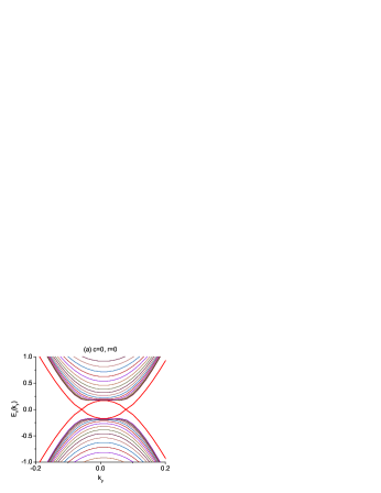
Since $\Gamma_{12}$ is conserved, the system is equivalent to a decoupled bilayer quantum Hall system, and the bulk Chern number defined for the Hamiltonian $H_{\Gamma_{12},1}(r=1,\theta_{x},\theta_{y})$ is $N=4$ for $0<e_{s}<4$, as shown in Ref.Qi et al. . According to the arguments in the last subsection, there should be gapless edge states in the open-boundary system, as verified numerically in Fig.3 (a).

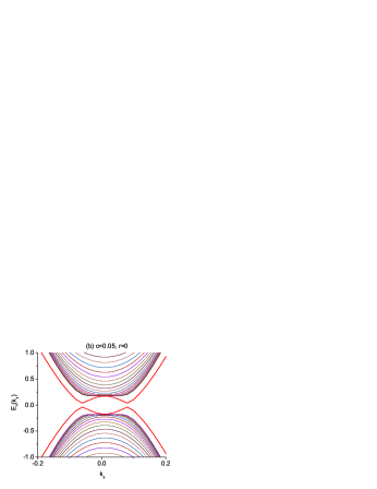
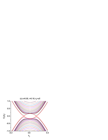
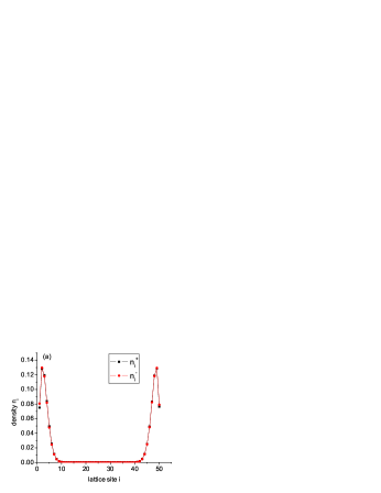
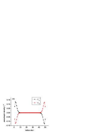
However, when $d_{1},d_{2}\neq 0$, the edge states in the system with open boundary conditions will become gapful with a gap of the order $\sqrt{d_{1}^{2}+d_{2}^{2}}$, since the $\Gamma_{1},\Gamma_{2}$ terms will mix the states with opposite $\Gamma_{12}$-eigenvalue. Also as long as $|d_{1}|,|d_{2}|\ll\sqrt{d_{\alpha}d^{\alpha}},\alpha=3,4,5$, the bulk gap cannot be closed by turning on $d_{1},d_{2}$. Consequently, the Berry phase gauge field remains well-defined on the torus with $r=1$, and thus the Chern number for the Hamiltonian $H_{\Gamma_{12}1}(r=1,\theta_{x},\theta_{y})$ remains unchanged. According to our Theorem 1, there must be some $(r\neq 0,\theta_{x},\theta_{y})$ where the system become gapless. Since all the twist transformations only make changes in the boundary terms in the Hamiltonian, it is reasonable to expect the gapless excitations to live around the edges. The nonzero tunnelling $r\neq 0$ between the edges actually mixes the original edge states to form new gapless excitations that are localized at the edge. To verify this, we have done a numerical calculation for the model with $c=0.05$. We identified two gapless points in parameter space at $r=0.18,\theta_{x}=\pm\pi/2,\theta_{y}=\pi$. The evolution of the band structure is shown in Fig. 3. At each gapless point there are two level crossings, which keeps the total winding number $4$. The charge and pseudo-spin density distributions of the gapless states are shown in Fig. 4, confirming that it is localized symmetrically around the edge, and the pseudo-spin polarization is opposite on the two sides of the edge.

Figure 4: The distribution of (a) charge density; (b) pseudo-spin $\Gamma_{12}$ density of the two edge states with wavevector $k=0.16\pi$ and with $c=0.05,r=0.18,\theta_{x}=\pi/2$.

III.3 Quantum Spin Hall Effect:
a Perturbative Study

It will be helpful to study how the gapless edge state arises from the original edge states through tunnelling in perturbation theory. Under the condition $|d_{1}|,|d_{2}|\ll\sqrt{d_{\alpha}d_{\alpha}}$ and $r\ll 1$, all the effects induced by nonzero $d_{1},d_{2}$ and by twisted boundary conditions are only significant for the edge states, while leading to little change in the bulk states. Thus it is reasonable to describe the low energy dynamics in an effective 1-d edge Hamiltonian. Let us first take the continuum limit of the gapless edge Hamiltonian for the system with $d_{1}=d_{2}=0,r=0$ as the starting point:

$$H^{\rm edge}_{0}=\sum_{s\alpha}\int dk\alpha vk\left(\phi^{\dagger}_{kLs\alpha}\phi_{kLs\alpha}-\phi^{\dagger}_{kRs\alpha}\phi_{kRs\alpha}\right),$$ (19)

in which $\alpha=\pm 1$ corresponds to the eigenvalue of $\Gamma_{12}$, and $L,R$ the states at the left and right edges. $s=1,2$ correspond to two crossings in Fig. 3 (a), and the wave-vector $k$ is defined in reference to the corresponding crossing points. The time reversal transformation of the 8 edge states is $T\phi_{k,L(R),1,\alpha}T^{-1}=\alpha\phi_{-k,L(R),2,-\alpha}$. When $r\neq 0$, we need to incorporate the mixing between different edges, and when $d_{1},d_{2}\neq 0$ the mixing between different $\alpha$. The states with different $s$ will never be mixed. So we take the perturbed effective Hamiltonian to be of the form

$$H_{\rm edge} = \int dk\alpha vk\left(\phi^{\dagger}_{kLs\alpha}\phi_{kLs\alpha}-\phi^{\dagger}_{kRs\alpha}\phi_{kRs\alpha}\right)$$ (20)

$$+ \int dk\left(u_{Ls}\phi_{kLs\uparrow}^{\dagger}\phi_{kLs\downarrow}+u_{Rs}\phi_{kRs\uparrow}^{\dagger}\phi_{kRs\downarrow}+h.c.\right)$$

$$+ r\sum_{s}\int dk\left(\phi_{kLs\alpha}^{\dagger}e^{i\theta\alpha}\phi_{kRs\alpha}+h.c.\right)$$

$$\equiv \sum_{s}\int dk\Phi^{\dagger}_{ksi}M^{s}_{ij}\Phi_{ksj},\qquad(i,j=1,\cdots,4)$$

in which $\Phi_{ks}=\left(\phi_{kLs\uparrow},\phi_{kLs\downarrow},\phi_{kRs\uparrow},\phi_{kRs\downarrow}\right)$. The matrix elements $u_{L(R)s}$ are defined as

$$u_{L(R)s}\equiv\left\langle k=0,L(R)s\uparrow\right|d_{1}\Gamma^{1}+d_{2}\Gamma^{2}\left|k=0,L(R)s\downarrow\right\rangle$$

where the $k$-dependence of the matrix elements is ignored. The matrix $M^{s}_{ij}$ is defined as

$$M^{s} = \left(\begin{array}[]{c c c c}vk&u^{*}_{Ls}&re^{i\theta}&0\\ u_{Ls}&-vk&0&re^{-i\theta}\\ re^{-i\theta}&0&-vk&u_{Rs}^{*}\\ 0&re^{i\theta}&u_{Rs}&vk\end{array}\right)\ .$$ (25)

Direct diagonalization of $M$ gives the four eigenvalues:

$$E_{s\alpha\beta}=\alpha\sqrt{v^{2}k^{2}+\frac{{|u_{Ls}|}^{2}+{|u_{Rs}|}^{2}}{2}+r^{2}+\beta\sqrt{\frac{\left({|u_{Rs}|}^{2}-{|u_{Ls}|}^{2}\right)^{2}}{4}+r^{2}\left({|u_{Ls}|}^{2}+{|u_{Rs}|}^{2}+2{|u_{Ls}|}{|u_{Rs}|}\cos 2\tilde{\theta}_{s}\right)}}\ ,$$ (26)

in which $\alpha,\beta=\pm 1$ and

$$\tilde{\theta}_{s}=\theta+{\rm Arg}(u_{Ls})-{\rm Arg}(u_{Rs})\ .$$

The equation $E_{s\alpha\beta}=0$ has two solutions:

$$\tilde{\theta}_{s}=0\text{ or }\pi,\qquad r=r_{s}\equiv\sqrt{|u_{Ls}u_{Rs}|}\ .$$ (27)

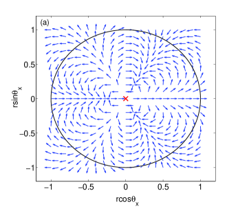
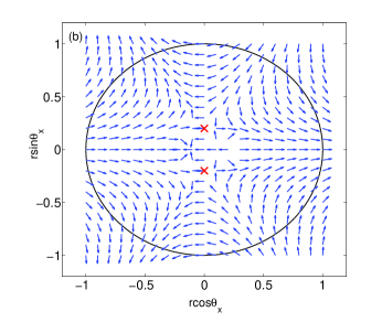
If $r_{1}\neq r_{2}$, there are 4 gapless points $(0,r_{1,2}),(\pi,r_{1,2})$ in the parameter space. In other words, the original singularity at $r=0$ with winding number $4$ is split to $4$ singularities each with unit winding number. However, the time reversal invariance will force $r_{1}=r_{2}$, since $\phi_{kL(R)1}$ are the T-partner of $\phi_{-kL(R)2}$. Therefore, the 4 singularities must merge to $2$, each with winding number 2, which is consistent with the above numerical results. The schematic picture of $\phi_{y}(r,\theta_{x})$ configurations for $c=0$ and $c\neq 0$ is shown in Fig. 5.

Concluding this section, we would like to emphasize that the existence of gapless edge states for a proper set of twisted boundary conditions with inter-edge tunnelling should not be viewed as a trivial result of fine tuning. For example, if one replaces the inter-edge tunnelling term in Eq. (20) by

$$r\sum_{s}\int dk\left(\phi_{kLs\alpha}^{\dagger}e^{i\theta}\phi_{kRs\alpha}+h.c.\right)\ ,$$

the Hamiltonian will be gapped for any $(r,\theta)$ as long as $u_{L,Rs}\neq 0$ and ${\rm Im}\left(u_{Ls}/u_{Rs}\right)\neq 0$, a direct consequence of the vanishing Chern number in the charge channel.

Figure 5: Schematic picture of the $\phi_{y}(r,\theta_{x})$ configuration for the spin Hall system when (a) $c=0$; (b) $c\neq 0$. The direction of the arrows stands for the phase $\phi_{y}$. The crosses indicate the position of singularities and the circle is the unit circle $r=1$.

IV Role of Time Reversal Invariance

Time reversal invariance plays an important role in the topological description of the quantum spin Hall systems. For the non-interacting fermion case, a $Z_{2}$ classification has been proposed in Ref.Kane and Mele (2005b), namely the gaplessness of edge states in open-boundary systems is protected by Kramers degeneracy, if there are in total an odd number pairs of edge states. However, the situation is very subtle when interactions are included in the many-body system. Below we will first show a consequences of time reversal invariance (Theorem 2) in a general many-body system in subsection A, and then discuss about the $Z_{2}$-classification in subsection B, where new predictions will be made based on Theorem 1.

IV.1 Conditions for Winding Number Doubling

For simplicity, we consider the case when $\Gamma_{x},\Gamma_{y}$ each carries a simple representation of time reversal transformation:

$$T\Gamma_{\mu}T^{-1}=\eta_{\mu}\Gamma_{\mu},\qquad\eta_{\mu}=\pm 1\ .$$ (28)

If the original Hamiltonian (1) is TR-invariant, then the TR property of the twisted Hamiltonian (5) will be

$$TH_{\Gamma_{x}\Gamma_{y}}(r,\theta_{x},\theta_{y})T^{-1}=H_{\Gamma_{x}\Gamma_{y}}(r,-\eta_{x}\theta_{x},-\eta_{y}\theta_{y})$$ (29)

Thus the gauge field has the symmetry property

$$A_{\mu}(r,\theta_{x},\theta_{y})=-i\left\langle G(r,\theta_{x},\theta_{y})\right|\partial_{\mu}\left|G(r,\theta_{x},\theta_{y})\right\rangle$$

$$=i\left\langle G(r,-\eta_{x}\theta_{x},-\eta_{y}\theta_{y})\right|\partial_{\mu}\left|G(r,-\eta_{x}\theta_{x},-\eta_{y}\theta_{y})\right\rangle$$

$$=\eta_{\mu}A_{\mu}(r,-\eta_{x}\theta_{x},-\eta_{y}\theta_{y}),$$

$$\Rightarrow F_{xy}(r,\theta_{x},\theta_{y})=-\eta_{x}\eta_{y}F_{xy}(r,-\eta_{x}\theta_{x},-\eta_{y}\theta_{y})\ .$$ (30)

Thus the Chern number $N$ is non-vanishing only when $\eta_{x}\eta_{y}=-1$. In the usual QHE case $\eta_{x}=\eta_{y}=1$, which means that the Hall conductivity vanishes for TR-invariant systems. On the other hand, the spin Hall effect corresponds to $\eta_{x}=-1$, $\eta_{y}=1$, since $\Gamma_{x}$ is a spin operator and $\Gamma_{y}=1$ is taken to be the charge operator. Below we will focus on the case with $\eta_{x}=-1,\eta_{y}=1$.

In general the first Chern number $N$ can be either even or odd integer. However, we will show that $N$ must be even when

$$e^{i\Gamma_{x}\pi}=-1\ .$$ (31)

When $\Gamma_{x}$ is a component of the spin operator, this condition simply means that the spin is a half-odd integer.

To prove this statement, it is convenient to introduce a deformed Hamiltonian by redefining the twisted boundary condition in the $x$-direction as

$$t_{ij}\rightarrow t_{ij}re^{i\Gamma_{x}\theta_{x}}e^{i\alpha_{x}},\qquad\left\langle ij\right\rangle\text{ across }L_{x}\,$$ (32)

and leaving the twisted boundary condition in the $y$-direction unchanged as in Eq.(4). In this way, we denote the auxiliary Hamiltonian as

$$H^{\prime}_{\Gamma_{x}\Gamma_{y}}\left(r,\theta_{x},\alpha_{x},\theta_{y}\right).$$ (33)

The introduction of the charge twist phase $e^{i\alpha_{x}}$ changes the TR property of $H^{\prime}$ to

$$TH^{\prime}_{\Gamma_{x}\Gamma_{y}}\left(r,\theta_{x},\alpha_{x},\theta_{y}\right)T^{-1}$$

$$=H^{\prime}_{\Gamma_{x}\Gamma_{y}}\left(r,\theta_{x},-\alpha_{x},-\theta_{y}\right)\ .$$ (34)

On the other hand, noticing the condition (31), we get

$$H^{\prime}_{\Gamma_{x}\Gamma_{y}}\left(r,\theta_{x},\alpha_{x},\theta_{y}\right)$$ (35)

$$= H^{\prime}_{\Gamma_{x}\Gamma_{y}}\left(r,\theta_{x}+\pi,\alpha_{x}+\pi,\theta_{y}\right).$$

Combining Eqs. (34) and (35) and taking $\alpha_{x}=\pi/2$, we obtain

$$TH^{\prime}_{\Gamma_{x}\Gamma_{y}}\left(r,\theta_{x},\frac{\pi}{2},\theta_{y}\right)T^{-1}$$

$$=H^{\prime}_{\Gamma_{x}\Gamma_{y}}\left(r,\theta_{x}+\pi,\frac{\pi}{2},-\theta_{y}\right)\ .$$ (36)

In the same way as for the Hamiltonian (5), the Berry phase gauge field $A_{\mu}^{\prime}$ and the phase factor $\phi^{\prime}(r,\theta_{x})=\int_{0}^{2\pi}A_{y}^{\prime}(r,\theta_{x},\theta_{y})d\theta_{y}$ can be defined for (the unique ground state of) $H^{\prime}$. Then Eq. (36) leads to the symmetry property

$$\phi^{\prime}(r,\theta_{x})=\phi^{\prime}(r,\theta_{x}+\pi),$$ (37)

which means $\phi^{\prime}$ is symmetric under the central reflection $(r,\theta)\rightarrow(r,\theta+\pi)$. Consequently, the positions of the singularities are also symmetric under the same transformation, thus the winding number must be even:

$$N^{\prime}(r) \equiv \int_{0}^{2\pi}\frac{\partial\phi^{\prime}(r,\theta_{x})}{\partial\theta_{x}}d\theta_{x}$$ (38)

$$= 2\int_{0}^{\pi}\frac{\partial\phi^{\prime}(r,\theta_{x})}{\partial\theta_{x}}d\theta_{x}=\text{even integer}\,$$

if the Hamiltonian $H^{\prime}_{\Gamma_{x}\Gamma_{y}}(r,\theta_{x},\frac{\pi}{2},\theta_{y})$ is gapped for all $\theta_{x},\theta_{y}\in[0,2\pi)$ at given $r$.

As the last step, the no-phase-stiffness condition is introduced again, which means the energy spectrum of the system is insensitive to $\alpha_{x}$ in the thermodynamic limit. Therefore, whenever $H^{\prime}_{\Gamma_{x}\Gamma_{y}}(r,\theta_{x},\frac{\pi}{2},\theta_{y})$ is gapped, the Hamiltonian (5),

$$H_{\Gamma_{x}\Gamma_{y}}(r,\theta_{x},\theta_{y})=H^{\prime}_{\Gamma_{x}\Gamma_{y}}(r,\theta_{x},0,\theta_{y}),$$

should also be gapped. This implies that the singularity distribution of $\phi(r,\theta_{x})$ is the same as that of $\phi^{\prime}(r,\theta_{x})$. As a result, the Chern number of the spin Hall system $H_{\Gamma_{x}\Gamma_{y}}(r,\theta_{x},\theta_{y})$ must be an even integer, and we have finally proved the following theorem:

• Theorem 2: If the conditions below are satisfied:

  1. $T\Gamma_{x}T^{-1}=-\Gamma_{x},T\Gamma_{y}T^{-1}=\Gamma_{y}$,

  2. $\exp(i\Gamma_{x}\pi)=-1$,

  3. the original Hamiltonian is TR-invariant, with charge conservation but without phase stiffness (i.e. without superconductivity),

  then the singularities in the phase field $\phi(r,\theta_{x})$ defined in Eq. (11) distribute symmetrically with respect to the origin $r=0$ on the $(r,\theta_{x})$-plane, and the Chern number for the unique ground state of $H_{\Gamma_{x}\Gamma_{y}}(r,\theta_{x},\theta_{y})$ is an even integer.

IV.2 Comments on $Z_{2}$ Classification

After studying the general consequence of time reversal invariance, now it is time to consider whether there is any additional topological classification besides the U(1) Chern number for TR-invariant systems. Although the singularities distribute symmetrically around the origin $r=0$ when the conditions in Theorem 2 are satisfied, it is still possible for all singularities to move away from the origin $r=0$, which means the edge states in the open-boundary system is not protected to be gapless. However, it has been shown analyticallyKane and Mele (2005a, b) and numericallySheng et al. (2005) that gapless edge states along the open boundaries in a spin Hall insulator model proposed for graphene remains robust against disorder. In Ref.Sheng et al. it is further shown that the existence of gapless edge states and the non-vanishing bulk Chern number $N=2$ in the spin channel are in one-to-one correspondence. The robustness of the gapless edge states in an open-boundary system comes from Kramers degeneracy, and applies only when there are an odd number of Kramers pairs on each edge, which corresponds to the Chern number $N=4n+2,n\in\mathbb{Z}$. In this way, a $Z_{2}$ classification is well-defined for non-interacting fermion systems, which distinguishes the spin Hall insulators with Chern number $N=4n+2$ from those with $N=4n$.

To generalize this mechanism to an interacting system, it should be noticed that the condition for Kramers degeneracy,

$$TTc_{k\alpha}T^{-1}T^{-1}=-c_{k\alpha},$$ (39)

is a single-particle property, not a condition on the many-body wave function. When interactions are taken into account, the gapless edge states emerging at some singular point $(r,\theta_{x})$ in parameter space may carry quantum numbers different from the constituent particle. Thus, the protection for Kramers degeneracy can survive only if the condition (39) is still true for the edge modes. Such a protection can be understood both by edge dynamics and by bulk topology. Below we will discuss about $Z_{2}$ classification from the bulk topology as a consequence of both Kramers degeneracy and Theorem 2.

To proceed, we introduce a conjecture that is known to be true for non-interacting systemsHatsugai (1993b), but has not been proven for a general many-body system:

• Conjecture: If there is a singularity of the $\phi(r,\theta_{x})$ field with winding number $N$ at some point $(r,\theta_{x})$, the corresponding Hamiltonian $H_{\Gamma_{x}\Gamma_{y}}(r,\theta_{x},\theta_{y})$ has $2N$ branches of gapless edge states.

Below we will take this conjecture as the starting point and leave its proof to future work. In accordance with this conjecture, a singularity with winding number $N=1$ corresponds to $2$ branches of edge modes. If the edge modes carry $T^{2}=-1$, the two branches must be $T$-conjugate to each other. Therefore there must be a Kramers degeneracy between them that cannot be broken by any perturbation without breaking the time reversal symmetry. Recall that the twist phase factor $e^{i\Gamma_{x}\theta_{x}}$ is T-even when $T\Gamma_{x}T^{-1}=-\Gamma_{x}$, the local variation of parameter $(r,\theta_{x})$ around the singular point can be considered as local perturbation respecting T-symmetry, which thus must maintain the system gapless. In other words, the system cannot have point-like singularity with winding number $N=1$ anywhere in the parameter space. A similar argument shows that all the point-like singularity in the ($r,\theta_{x}$)-plane with $N$ odd is forbidden. Consequently, all the vortex-like singularities of the $\phi(r,\theta_{x})$ field has an even winding number. Taking into account the central reflection symmetry of the singular points as a corollary of Theorem 2, we know that all the singularities away from $r=0$ provide a winding number $4n$. Thus at least $2$ pairs of gapless edge states must exist for an open-boundary system when the bulk Chern number is $N=4n+2,\ (n\in\mathbb{Z})$.

In summary, the $Z_{2}$ classification is applicable when the system satisfies all the conditions of Theorem 2 and also has all its low-energy quasiparticles odd under $T^{2}$-operation. It should be clarified that for an interacting system, the condition (31) does not imply $T^{2}=-1$ for low-lying modes. Since the properties of low-energy quasiparticles may change without closing the bulk gap, there seems no reason to believe the $Z_{2}$ “order” is protected by the bulk topology alone; it rather depends on the detail of interactions.

From the discussion above, new predictions can be obtained for the $N=1$ system. In Ref.Wu et al. (2006); Xu and Moore (2006), the edge dynamics for some $N=1$ systems has been studied, which shows that the edge states in the open-boundary system can be gapped with proper interactions. After such a gap is opened, there are two possibilities for this system:

1. As shown in Ref.Wu et al. (2006), the ground state of an open-boundary system may break time reversal symmetry spontaneously, which leads to ground state degeneracy. In this case, the point $r=0$ is still singular. If the Chern number $N=2$ is still carried by this singularity, then no other singularity necessarily exists.
   

2. If the singularity at $r=0$ does not carry any Chern number, or if the TR-symmetry is recovered, then the bulk topology requires the gapless edge states to exist with proper inter-edge tunnelling strength. What’s more, from the discussion in this subsection we know that as long as the gapless edge states shift to $r\neq 0$, they must be even under $T^{2}$ operation. Physically, this prediction means that before the gap-opening transition, the edge modes are $T^{2}$-odd quasi-particles, which carry similar quantum numbers as free fermions; immediately after this transition, the edge modes will become $T^{2}$-even, which may correspond to some kind of spin and/or charge density waves.

V Summary and Discussions

In conclusion, in this paper we have established, for 2d insulators, a general connection between bulk topological order and edge dynamics illustrated by Theorem 1. The key idea behind demonstrating this bulk-edge relation is to bring in an additional parameter that describes the strength of edge tunnelling besides the twisted boundary phases introduced in Ref.Niu et al. (1985). This results in a three dimensional parameter space and implements a continuous interpolation between a cylindrical system with open boundaries and a toroidal system. In this framework, it is clarified that generically the bulk topological order for an insulator in torus geometry is not necessarily associated with gapless edge states in cylinder geometry. On the one hand, the the emergence of gapless edge states known for QH systems is shown to be closely related to charge conservation in addition to topological reasons. On the other hand, a QSH system with non-trivial bulk Chern number and gapped edge states is predicted to have gapless edge states when inter-edge tunnelling with proper strength is turned on. Finally, a general consequence of time reversal invariance is deduced in Theorem 2. The $Z_{2}$ classification is shown to be dependent, besides bulk topology, also on the $T^{2}$ ($T$ being time reversal) quantum number of relevant low-lying modes, which is not topological in nature and can be changed by interactions without changing the bulk topological order.

The proof of Theorem 1 can in principle be generalized to topological insulators in higher dimensions, for which the topological order is related to non-Abelian Berry phase gauge field and higher Chern numbers. For example, in the four dimensional quantum Hall effectZhang and Hu (2001), the second Chern number can be defined when the Berry phase gauge field is ${\rm SU(N)}$ and the parameter space is 4-dimensional as labeled by $(\theta_{x},\theta_{y},\theta_{z},\theta_{w})$. In the same way as in Sec. II, an amplitude $r$ can be introduced for any boundary and a non-Abelian Berry phase field $U(r,\theta_{\mu})\in{\rm SU(N)}$ can be defined by a straightforward generalization of Eq. (11) to a Wilson loop operator:

$$\Phi(r,\theta_{\mu})=P\exp\left[i\int A_{w}(r,\theta_{x},\theta_{y},\theta_{z},\theta_{w})d\theta_{w}\right],$$ (40)

in which $\mu=x,y,z$ and $P$ stands for path ordering. The second Chern number is then identified as the winding number of the $U$ field on the 3-torus $T^{3}$ at $r=1$. By the same topological reasoning, there must be singularities of the $U$ field for some $(r,\theta_{\mu})$ with $r<1$ when the bulk Chern number for the system with $r=1$ is non-trivial, which corresponds to gapless edge states in higher dimensional sense. In this way, Theorem 1 provides a universal modus operandi to understand the bulk-edge relationship in topological insulators.

This work is supported in part by the NSFC through the grants No. 10374058, and by the US NSF through the grants PHY-0457018 and DMR-0342832, and by the US Department of Energy, Office of Basic Energy Sciences under contract DE-AC03-76SF00515. We would like to acknowledge helpful discussions with B. A. Bernevig, J. P. Hu, C. Kane, J. Moore, D. N. Sheng, Z. Y. Weng, C. J. Wu and C. K. Xu.

References

- von Klitzing et al. (1980) K. von Klitzing, G. Dorda, and M. Peper, Phys. Rev. Lett. 45, 494 (1980).
- Thouless et al. (1982) D. J. Thouless, M. Kohmoto, M. P. Nightingale, and M. den Nijs, Phys. Rev. Lett. 49, 405 (1982).
- Volovik (2003) G. Volovik, The universe in a helium droplet (Oxford Publications, Oxford, 2003).
- Niu et al. (1985) Q. Niu, D. J. Thouless, and Y.-S. Wu, Phys. Rev. B 31, 3372 (1985).
- Laughlin (1981) R. B. Laughlin, Phys. Rev. B 23, 5632 (1981).
- Halperin (1982) B. I. Halperin, Phys. Rev. B 25, 2185 (1982).
- Hatsugai (1993a) Y. Hatsugai, Phys. Rev. B 48, 11851 (1993a).
- Hatsugai (1993b) Y. Hatsugai, Phys. Rev. Lett. 71, 3697 (1993b).
- Murakami et al. (2003) S. Murakami, N. Nagaosa, and S.-C. Zhang, Science 301, 1348 (2003).
- Sinova et al. (2004) J. Sinova, D. Culcer, Q. Niu, N. A. Sinitsyn, T. Jungwirth, and A. H. MacDonald, Phys. Rev. Lett. 92, 126603 (2004).
- Murakami et al. (2004) S. Murakami, N. Nagaosa, and S.-C. Zhang, Phys. Rev. Lett. 93, 156804 (2004).
- Kane and Mele (2005a) C. L. Kane and E. J. Mele, Phys. Rev. Lett. 95, 226801 (2005a).
- Bernevig and Zhang (2006) B. A. Bernevig and S.-C. Zhang, Phys. Rev. Lett. 96, 106802 (2006).
- (14) X.-L. Qi, Y.-S. Wu, and S.-C. Zhang, cond-mat/0505308.
- Sheng et al. (2005) L. Sheng, D. N. Sheng, C. S. Ting, and F. D. M. Haldane, Phys. Rev. Lett. 95, 136602 (2005).
- Hatsugai (2005) Y. Hatsugai, J. Phys. Soc. Jap. 74, 1374 (2005).
- (17) Y. Hatsugai, T. Fukui, and H. Suzuki, cond-mat/0507466.
- (18) D. N. Sheng, Z. Y. Weng, L. Sheng, and F. D. M. Haldane, cond-mat/0603054.
- Kane and Mele (2005b) C. L. Kane and E. J. Mele, Phys. Rev. Lett. 95, 146802 (2005b).
- Wu et al. (2006) C. Wu, B. A. Bernevig, and S.-C. Zhang, Phys. Rev. Lett. 96, 106401 (2006).
- Xu and Moore (2006) C. Xu and J. E. Moore, Phys. Rev. B 73, 045322 (2006).
- Wu (1990; pp. 461-491) Y. Wu, Lectures on “Topological Aspests of the Quantum Hall Effect”, in “Physics, Geometry and Topology” (Proceedings of Banff NATO Summer School in Theoretical Physics, Banff, Canada (Aug. 14-25, 1989); ed. by H.C. Lee, Plenum Press (New York and London), 1990; pp. 461-491).
- Kohmoto (1985) M. Kohmoto, Annals of Physics 160, 355 (1985).
- Zhang and Hu (2001) S.-C. Zhang and J. Hu, Science 294, 823 (2001).