Phonon spectral function of the Holstein polaron

Abstract

The phonon spectral function of the one-dimensional Holstein model is obtained within weak and strong-coupling approximations based on analytical self-energy calculations. The characteristic excitations found in the limit of small charge-carrier density are related to the known (electronic) spectral properties of Holstein polarons such as the polaron band dispersion. Particular emphasis is laid on the different physics occurring in the adiabatic and anti-adiabatic regimes, respectively. Comparison is made with a cluster approach exploiting exact numerical results on small systems to yield an approximation for the thermodynamic limit. This method, similar to cluster perturbation theory, confirms the analytical findings, and yields accurate results also in the intermediate-coupling regime.

1 Introduction

Intermediate or strong electron-phonon (EP) interaction gives rise to the existence of polaronic carriers in a number of interesting materials (see, e.g., [1, 2, 3]). As a consequence, models for such quasiparticles, e.g., the Holstein model [4] considered here, have been investigated intensively in the past decades in order to understand the process of polaron formation. Whereas valuable insight into the latter may be gained by considering a single charge carrier (i.e., the Holstein polaron problem), real materials are usually characterized by finite carrier densities, motivating studies of many-polaron models [5, 6, 7, 8].

Over the last decade, a large number of theoretical studies, the most reliable of which based on unbiased numerical methods, have led to a fairly complete understanding of the Holstein polaron concerning both ground-state and spectral properties. Calculations of the latter, e.g., the one-electron Green function, are particularly rewarding as they provide detailed insight into the non-linear process of an electron becoming self-trapped in the surrounding lattice distortion. For reviews of the Holstein polaron problem see [9, 10].

In this paper, we contribute to a completion of the knowledge about the single-polaron problem by investigating the phonon spectral function, an important observable rarely considered in previous work. On the contrary, it has been studied quite intensively for the spinless Holstein model and the Holstein-Hubbard model, both at half filling, for which phonon softening at the zone boundary has been found to occur at the Peierls transition in one dimension [11, 12, 13, 14, 15, 16]. Note that the assumption of a local self-energy frequently used in combination with dynamical mean field theory (DMFT)—as appropriate for infinite dimensions—leads to an unrealistic wavevector-independent softening of all phonon excitations [17, 18]. The renormalization of the phonon modes in small clusters with one electron, especially their softening at the critical EP coupling, has been investigated numerically in [19], and results for the coherent phonon spectrum of the infinite system have been reported in [20]. Furthermore, analytical approximations for the phonon self-energy and the frequencies of the vibration modes in the coupled EP system have been obtained in [21, 22, 5].

Here we present analytical calculations valid at weak and strong EP coupling, respectively, as well as a cluster approach, similar to cluster perturbation theory [23, 24, 25], which yields accurate results in all relevant parameter regimes. Both approaches are capable of describing the momentum dependence of the phonon spectral functions, and we find a very good agreement between analytical and numerical results.

Despite the formal restriction to the one-electron case, the numerical results will correspond to finite electron densities due to the finite underlying clusters. The analytical calculations presented here are based on the electron (polaron) spectral functions previously deduced in [26] for the weak-coupling (WC) and strong-coupling (SC) cases and for charge carrier concentrations $n<0.5$. These spectral functions depend on $n$ and their calculation requires a self-consistent determination of the chemical potential $\mu$. To avoid this difficult task, we shall consider the analytical formulas in the mathematical limit of $\mu$ approaching the bottom of the electron (polaron) band. The resulting limiting shape of the spectral functions will provide us with a picture of the phonon spectrum for small carrier concentrations. In particular, as demonstrated below, the positions of the low-energy excitations will be found to be in a very good agreement with numerical results. Moreover, the general analytical treatment will enable us to discuss to some extent the features which occur for non-negligible carrier concentrations.

The paper is organized as follows. In section 2, we introduce the Holstein model. Section 3 is devoted to the derivation of the analytical results and a discussion of our cluster approach, whereas section 4 contains the results and a discussion. Finally, we summarize in section 5.

2 Model

In view of the SC approximation presented below, it is convenient to write the Hamiltonian of the one-dimensional (1D) spinless Holstein model as

$$H=-\mu\sum_{j}\hat{n}_{j}+\omega_{0}\sum_{j}b^{\dagger}_{j}b^{\phantom{{\dagger}}}_{j}-\sum_{jj^{\prime}}C^{\phantom{{\dagger}}}_{j^{\prime}j}c^{\dagger}_{j^{\prime}}c^{\phantom{{\dagger}}}_{j}\,,$$ (1)

where

$$C_{jj}=g\omega_{0}(b^{\dagger}_{j}+b^{\phantom{{\dagger}}}_{j})\,,\quad C_{\langle j^{\prime}j\rangle}=t\,.$$ (2)

In equation (1), $c^{\dagger}_{i}$ ($b^{\dagger}_{i}$) creates a spinless fermion (a phonon of energy $\omega_{0}$) at site $i$, and $\hat{n}_{i}=c^{\dagger}_{i}c^{\phantom{{\dagger}}}_{i}$ with $n_{i}=0,1$. The first term contains the chemical potential $\mu$ and determines the carrier density $n$, whereas the second term accounts for the elastic and kinetic energy of the lattice. Finally, the last term describes the local coupling between the lattice displacement $x_{i}=b^{\dagger}_{i}+b^{\phantom{{\dagger}}}_{i}$ and the electron density $\hat{n}_{i}$ with the coupling parameter $g$ (for $j=j^{\prime}$, cf equation (2)), as well as electron hopping processes between neighbouring lattice sites $\langle j^{\prime}j\rangle$ with hopping amplitude $t$ (for $j=j^{\prime}\pm 1$). We take $t$ as the unit of energy, and set the lattice constant to unity.

From numerous previous investigations [10] of this model in the one-electron case considered here the following picture emerges. At WC, the ground state consists of a large polaron, corresponding to a self-trapped electron with a lattice distortion extending over many lattice sites. As the EP coupling is increased, a cross-over takes place to a small-polaron state, in which the lattice distortion is essentially localized at the site of the electron, leading to a substantial increase of the quasiparticle’s effective mass in the intermediate-coupling (IC) and SC regime. Depending on the value of the adiabaticity ratio $\alpha=\omega_{0}/t$, the small-polaron cross-over occurs at a critical value of the EP coupling determined by the more restrictive of the two conditions $\lambda=E_{\mathrm{p}}/2t\geq 1$ (relevant for $\alpha\ll 1$) or $g^{2}=E_{\mathrm{p}}/\omega_{0}\geq 1$ (for $\alpha\gg 1$). Here $E_{\mathrm{p}}=g^{2}\omega_{0}$ is the polaron binding energy in the atomic limit defined by $t=0$.

3 Methods

3.1 Analytical approach

The aim of the present treatment is to deduce and to interpret the essential features of the numerically calculated phonon spectral functions (see section 4). In the following calculations, we shall deal with coupled equations of motion of the Matsubara Green functions for the lattice-oscillator coordinates on the one hand, and for the spinless charge carriers on the other hand. It will be shown that the general features of the spectral functions may be understood on the basis of the results obtained for the WC and SC cases, where an approximate treatment is well justified [7, 26].

3.1.1 Weak-coupling approximation

The Matsubara Green function for phonons, defined as

$$D(m_{1}\tau_{1};m_{2}\tau_{2})=-\langle T_{\tau}x_{m_{1}}(\tau_{1})x_{m_{2}}(\tau_{2})\rangle\,,$$ (3)

fulfills the equation of motion

$$\frac{1}{2\omega_{0}}\left(\frac{\partial^{2}}{\partial\tau_{1}^{2}}-\omega_{0}^{2}\right)D(m_{1}\tau_{1};m_{2}\tau_{2}) = \delta_{m_{1}m_{2}}\delta(\tau_{1}-\tau_{2})$$

$$-g\omega_{0}\langle T_{\tau}c^{\phantom{{\dagger}}}_{m_{1}}(\tau_{1})c^{\dagger}_{m_{1}}(\tau_{1})x_{m_{2}}(\tau_{2})\rangle\,,$$

assuming $\langle x_{m_{2}}\rangle=0$ in the WC regime. The mixed Green function on the rhs of equation (3.1.1) will be expressed by means of the generalized fermionic Green function [27, 28]

$$G(n_{1}\tau_{1};n_{2}\tau_{2};U)=-\frac{1}{\langle S\rangle}\langle T_{\tau}c^{\phantom{{\dagger}}}_{n_{1}}(\tau_{1})c^{\dagger}_{n_{2}}(\tau_{2})S\rangle\equiv G(1;2;U)$$ (5)

and

$$S=T_{\tau}\exp\left(-\int_{0}^{\beta}\rmd\tau\sum_{nn^{\prime}}U_{nn^{\prime}}(\tau)C_{nn^{\prime}}(\tau)\right)\,,$$ (6)

where the classical variables $U_{nn^{\prime}}(\tau)$ were introduced as a purely formal device. Consequently, the relation between the mixed Green function and the fermionic Green function reads

$$\quad\quad\quad\langle T_{\tau}c^{\phantom{{\dagger}}}_{n_{1}}(\tau_{1})c^{\dagger}_{n_{1}^{\prime}}(\tau_{1}^{\prime})C_{m_{2}m_{2}}(\tau_{2})\rangle=\left[\frac{\delta}{\delta U_{m_{2}m_{2}}(\tau_{2})}G(n_{1}\tau_{1};n_{1}^{\prime}\tau_{1}^{\prime};U)\right]_{U=0}\,.$$ (7)

Here $\delta/\delta U$ denotes the functional derivative. Defining the inverse Green function $G^{-1}(1;2;U)$ to $G(1;2;U)$ according to [27] we obtain

$$\langle T_{\tau}c^{\phantom{{\dagger}}}_{m_{1}}(\tau_{1})c^{\dagger}_{m_{1}}(\tau_{1})C_{m_{2}m_{2}}(\tau_{2})\rangle$$ (8)

$$=-\int_{0}^{\beta}\rmd\tau^{\prime\prime}\sum_{m^{\prime\prime}}G(m_{1}\tau_{1};m^{\prime\prime}\tau^{\prime\prime})$$

$$\quad\times\int_{0}^{\beta}\rmd\tau^{\prime}\sum_{m^{\prime}}\left[\frac{\delta}{\delta U_{m_{2}m_{2}}(\tau_{2})}G^{-1}(m^{\prime\prime}\tau^{\prime\prime};m^{\prime}\tau^{\prime};U)\right]_{U=0}G(m^{\prime}\tau^{\prime};m_{1}\tau_{1})$$

for the interaction term in the equation of motion (3.1.1). The resulting equation for the phonon Green function is quite general, as no approximations have been made up to now.

In the sequel, the fermionic Green functions in equation (8) will be obtained using the fermionic spectral functions $A(k,\omega)$ which have been calculated to second order in the EP coupling constant in [26]. To the same order, the functional derivative of $G^{-1}$ will be determined using the relation between the inverse Green function and the self-energy $\Sigma$, $G^{-1}(1;2;U)=G^{-1}_{0}(1;2)-\Sigma(1;2;U)$, where the Green function of the zeroth order, $G_{0}$, is independent of $U$. Accordingly, the derivative of $G^{-1}$ in equation (8) will be expressed as the derivative of $\Sigma$, which gives to second order [26, 29, 30]

$$\left[\frac{\delta}{\delta U_{m_{2}m_{2}}(\tau_{2})}\Sigma(m^{\prime\prime}\tau^{\prime\prime};m^{\prime}\tau^{\prime};U)\right]_{U=0}=\langle T_{\tau}C_{m^{\prime\prime}m^{\prime}}(\tau^{\prime\prime})C_{m_{2}m_{2}}(\tau_{2})\rangle\delta_{m^{\prime\prime}m^{\prime}}\delta(\tau^{\prime\prime}-\tau^{\prime})\,.$$ (9)

Therefore, equation (3.1.1) acquires the following form:

$$\frac{1}{2\omega_{0}}\left(\frac{\partial^{2}}{\partial\tau_{1}^{2}}-\omega_{0}^{2}\right)D(m_{1}\tau_{1};m_{2}\tau_{2}) = \delta_{m_{1}m_{2}}\delta(\tau_{1}-\tau_{2})-\int_{0}^{\beta}\rmd\tau^{\prime}\sum_{m^{\prime}}G(m_{1}\tau_{1};m^{\prime}\tau^{\prime})$$

$$\times\langle T_{\tau}C_{m^{\prime}m^{\prime}}(\tau^{\prime})C_{m_{2}m_{2}}(\tau_{2})\rangle G(m^{\prime}\tau^{\prime};m_{1}\tau_{1})\,.$$

However,

$$\quad\langle T_{\tau}C_{m^{\prime}m^{\prime}}(\tau^{\prime})C_{m_{2}m_{2}}(\tau_{2})\rangle=g^{2}\omega_{0}^{2}\langle T_{\tau}x_{m^{\prime}}(\tau^{\prime})x_{m_{2}}(\tau_{2})\rangle=-g^{2}\omega_{0}^{2}D(m^{\prime}\tau^{\prime};m_{2}\tau_{2})\,.$$ (11)

Substitution of equation (11) into equation (3.1.1) and subsequent multiplication on the rhs by $D^{-1}$ give

$$\Pi(m_{1}\tau_{1};m_{2}\tau_{2})=g^{2}\omega_{0}^{2}G(m_{1}\tau_{1};m_{2}\tau_{2})G(m_{2}\tau_{2};m_{1}\tau_{1})$$ (12)

with $\Pi=D_{0}^{-1}-D^{-1}$, the self-energy of the phonons in the Matsubara framework.

Fourier transformation of equation (12) leads to

$$\Pi(q,\rmi\omega_{n})=g^{2}\omega_{0}^{2}\frac{1}{N}\sum_{k}\frac{1}{\beta}\sum_{\nu}G(k,\rmi\omega_{\nu})G(k+q,\rmi(\omega_{\nu}+\omega_{n}))\,,$$ (13)

where $\omega_{\nu}=(2\nu+1)\pi/\beta$ and $\omega_{n}=2n\pi/\beta$ are Matsubara frequencies for fermions and bosons, respectively.

The substitution of the spectral representation of the fermionic Green functions

$$G(k^{\prime},\rmi\omega_{\nu})=\int_{-\infty}^{\infty}\,\rmd\omega^{\prime}\frac{A(k^{\prime},\omega^{\prime})}{\rmi\omega_{\nu}-\omega^{\prime}}$$ (14)

into equation (13), the summation over the frequencies $\omega_{\nu}$, the analytical continuation $\rmi\omega_{n}\mapsto\overline{\omega}=\omega+\rmi\delta$ and the subsequent limit $\delta\to 0$ lead to

$$\Pi(q,\omega+\rmi 0^{+}) = g^{2}\omega_{0}^{2}\frac{1}{N}\sum_{k}\int_{-\infty}^{\infty}\rmd\omega^{\prime}\int_{-\infty}^{\infty}\rmd\epsilon^{\prime}A(k,\omega^{\prime})$$ (15)

$$\times A(k+q,\epsilon^{\prime})[f(\omega^{\prime})-f(\epsilon^{\prime})]\zeta(\omega+\omega^{\prime}-\epsilon^{\prime})$$

with

$$f(x)=\frac{1}{\rme^{\beta x}+1}\,,\quad\zeta(x)=\frac{\mathcal{P}}{x}-\rmi\pi\delta(x)\,.$$ (16)

In the low-temperature limit the integrand of equation (15) may be non-zero only if

$$\omega^{\prime}<0\; \mathrm{and}\; \epsilon^{\prime}>0\Leftrightarrow f(\omega^{\prime})-f(\epsilon^{\prime})=1\quad\mathrm{or}$$

$$\omega^{\prime}>0\; \mathrm{and}\; \epsilon^{\prime}<0\Leftrightarrow f(\omega^{\prime})-f(\epsilon^{\prime})=-1\,.$$ (17)

Using the second-order result for the electron spectral function $A(k^{\prime},\omega^{\prime})$ deduced in [26], the calculation of the phonon self-energy (15), the corresponding retarded phonon Green function $D^{\mathrm{R}}(q,\omega)$ and the phonon spectral function $B(q,\omega)$ would be straight forward [31]. However, $A(k^{\prime},\omega^{\prime})$ as derived in [26] depends on the charge-carrier concentration $n$ and has to be determined self-consistently with a condition for the chemical potential $\mu$. The situation is thus simplified if we restrict ourselves to the case of small carrier concentration, for which the dependence on $n$ is expected to be unimportant. To choose the dominant contributions to the integral on the rhs of equation (15) for small $n$, the integration over $\omega^{\prime}$ and $\epsilon^{\prime}$ will be divided according to the character of the electronic spectral functions $A(k,\omega^{\prime})$ and $A(k+q,\epsilon^{\prime})$.

The coherent part of the spectrum $A_{\mathrm{c}}(k,\omega)$, non-zero for $|\omega|<\omega_{0}$, consists of quasiparticle peaks,

$$A_{\mathrm{c}}(k,\omega)=z_{k}\delta(\omega-(E_{k}-\mu))\,,$$ (18)

whereas outside this frequency interval the incoherent spectral function $A_{\mathrm{ic}}(k,\omega)$ is formed by peaks of finite width. In the sequel, the integrals obtained in this way will be examined with respect to the behaviour in the limit of small concentrations, i.e., for $\mu$ lying near $E_{0}$, the bottom of the band defined by equation (18).

The real and imaginary parts of $\Pi(q,\omega)$ are obtained if the real and imaginary parts of the $\zeta$-function are substituted into equation (15). The behaviour of the resulting integrals for $\mu$ in the neighbourhood of $E_{0}$ is then analyzed in the mathematical limit $\mu\to E_{0}^{+}$. We find that the integration for $\mathrm{Re}\,\Pi(q,\omega)$ according to equation (15) gives zero in the limit of vanishing carrier concentration. In contrast, the integration for $\mathrm{Im}\,\Pi(q,\omega)$ yields a non-zero result in this limit, with the coherent parts of the spectra, $A_{\mathrm{c}}(k,\omega^{\prime})$ and $A_{\mathrm{c}}(k+q,\epsilon^{\prime})$, being the only non-vanishing contributions. Taking into account only the latter, we shall express $\mathrm{Im}\,\Pi(q,\omega)$ as

$$\mathrm{Im}\,\Pi(q,\omega) = -\frac{1}{2}g^{2}\omega_{0}^{2}\int_{-\pi}^{\pi}\rmd kz_{k}z_{k+q}\delta(\omega-(E_{k+q}-E_{k}))\theta(\mu-E_{k})$$ (19)

$$\times\int_{0}^{\omega_{0}}\rmd\epsilon^{\prime}\delta(\epsilon^{\prime}-(E_{k+q}-\mu))$$

$$= -\frac{1}{2}g^{2}\omega_{0}^{2}\int_{|k|<k_{\mathrm{F}}}\rmd kz_{k}z_{k+q}\theta(\mu-E_{k})\frac{\delta(k-k_{0})}{|E^{\prime}_{k_{0}}-E^{\prime}_{k_{0}+q}|}$$

$$\times\int_{0}^{\omega_{0}}\rmd\epsilon^{\prime}\delta(\epsilon^{\prime}-(E_{k+q}-\mu))\,,$$

with $E_{k}\leq\mu<E_{k+q}<\omega_{0}$. According to [26], the energies of the electronic band are given by the equation

$$E_{k}=\xi_{k}+\frac{g^{2}\omega_{0}^{2}}{\pi W}\mathcal{P}\int_{-W}^{W}\frac{\rmd\xi}{\sqrt{1-(\xi/W)^{2}}}\frac{1}{E_{k}-\omega_{0}-\xi}\,,$$ (20)

where $\xi_{k}=-W\cos k$ ($W=2t$), and its derivative

$$E_{k}^{\prime}=Wz_{k}\sin k\,,$$ (21)

with the spectral weight [26]

$$z_{k}=\left|1+\frac{g^{2}\omega_{0}^{2}}{\pi W}\mathcal{P}\int_{-W}^{W}\frac{\rmd\xi}{\sqrt{1-(\xi/W)^{2}}}\frac{1}{(E_{k}-\omega_{0}-\xi)^{2}}\right|^{-1}\,.$$ (22)

The wavevector $k_{0}$ in equation (19) lies in the neighbourhood of $k=0$ defined by $\theta(\mu-E_{k})=1$ and satisfies

$$\omega-E_{k+q}+E_{k}=0\,.$$ (23)

Consequently, the value of $k_{0}$ appears to be a function of $\omega$ at fixed wavevector $q$, fulfilling $E_{k_{0}}<\mu$.

To obtain a qualitative picture of the phonon spectral function, we explicitly take the limit $\mu\to E^{+}_{0}$. Thereby, $\lim_{\mu\to E^{+}_{0}}\mathrm{Re}\,\Pi(q,\omega)=0$ and the rhs of equation (19) is non-zero only on the curve $\omega=\omega_{q}=E_{q}-E_{0}$ provided that $0<\omega<\omega_{0}$. The values of $\mathrm{Im}\,\Pi(q,\omega)$ are given as follows:

$$\quad\quad\quad\mathrm{Im}\,\Pi(q,\omega)=-\frac{1}{2}g^{2}\omega_{0}^{2}\frac{z_{0}}{W|\sin q|}\theta(\omega_{0}-(E_{q}-E_{0}))\Delta(\omega-(E_{q}-E_{0}))\,,$$ (24)

where the function $\Delta(x_{1}-x_{2})$ is the generalization of the Kronecker symbol being equal to unity for $x_{1}=x_{2}$ and zero otherwise. Consequently, in this limit, the narrow peaks of finite frequency width following for $\mathrm{Im}\,\Pi(q,\omega)$ from equation (19), are replaced by discrete lines given by equation (24). The divergence of the imaginary part of the phonon self-energy at $q=0$ and $q=\pi$ is connected with the 1D electron band dispersion. Our method of calculation only takes into account contributions to the electronic spectral function up to second order, which is insufficient if divergences occur.

On physical grounds, one expects no renormalization of the phonon excitations in the zero-density limit, i.e., for one electron in an infinite lattice. The non-zero imaginary part of the phonon self-energy even for $n\to 0$ [equation (24)] does not contradict this expectation since the integrated weight of the corresponding features is zero. As discussed in section 4, these non-zero contributions to the limit of the phonon spectrum may be related to results for small but finite carrier densities.

So far, we have restricted ourselves to $\omega>0$, but the case $\omega<0$ may be treated quite analogously. The only non-zero contribution to $\mathrm{Im}\,\Pi(q,\omega)$ in the limit $\mu\rightarrow E_{0}^{+}$ is obtained for $E_{k+q}<\mu<E_{k}<\omega_{0}$ in the frequency range $-\omega_{0}<\omega<0$ on the curve $\omega_{q}=-(E_{q}-E_{0})$, with the result

$$\mathrm{Im}\,\Pi(q,\omega)=-\mathrm{Im}\,\Pi(q,|\omega|)\,.$$ (25)

The retarded Green function $D^{\mathrm{R}}(q,\omega+\rmi\delta)$ as the analytical continuation of

$$D(q,\rmi\omega_{n})=\frac{2\omega_{0}}{(\rmi\omega_{n})^{2}-\omega_{0}^{2}-2\omega_{0}\Pi(q,\rmi\omega_{n})}$$ (26)

in the upper complex half-plane determines the phonon spectral function

$$B(q,\omega)=-\frac{1}{\pi}\mathrm{Im}\,D^{\mathrm{R}}(q,\omega+\rmi 0^{+})\,.$$ (27)

Using equation (26) and the preceding analysis of $\Pi(q,\omega+\rmi 0^{+})$ in the limit $\mu\rightarrow E_{0}^{+}$, we may conclude that for $\omega>0$

$$B(q,\omega)=-\frac{1}{\pi}\frac{(2\omega_{0})^{2}\mathrm{Im}\,\Pi(q,\omega)}{(\omega^{2}-\omega_{0}^{2})^{2}+[2\omega_{0}\mathrm{Im}\,\Pi(q,\omega)]^{2}}$$ (28)

if $\omega=E_{q}-E_{0}$ and $0<\omega<\omega_{0}$, where $\mathrm{Im}\,\Pi$ is given by equation (24). Otherwise $\mathrm{Im}\,\Pi(q,\omega>0)=0$ and

$$B(q,\omega)=\delta(\omega-\omega_{0})\,.$$ (29)

The result for $\omega<0$, analogous to equations (28), (29) fulfills the relation

$$B(q,\omega)=-B(q,-\omega)\,,$$ (30)

in agreement with the general requirement on the imaginary parts of retarded Green functions of real dynamical variables [32].

3.1.2 Strong-coupling approximation

The equation of motion (3.1.1) does not hold exactly in the SC regime, as the coordinate $x_{m}$ of the local oscillator at site $m$ implies a shift due to the local lattice deformation associated with on-site small-polaron formation. In fact, $\langle x_{m}\rangle=2g\langle c^{\dagger}_{m}c^{\phantom{{\dagger}}}_{m}\rangle$, which follows from the Lang-Firsov canonical displacement transformation [33]. However, dealing with the limit of negligible charge-carrier concentration, $\langle x_{m}\rangle=0$ may again be assumed. On the other hand, the charge-carrier number operator in the electron picture is equal to the number operator in the small-polaron picture. Therefore, we interpret the Fermi operators $c^{\phantom{{\dagger}}}_{m_{1}}(\tau_{1})$, $c^{\dagger}_{m_{1}}(\tau_{1})$ in equation (3.1.1) as annihilation and creation operators of small polarons—the correct quasiparticles in the SC limit. Accordingly, the mixed term on the rhs of equation (3.1.1) will be expressed using the generalized small-polaron Green functions, defined again by equations (5), (6), where the operators $C_{nn}(\tau)=g\omega_{0}x_{n}(\tau)$ as before, but the $C_{\langle nn^{\prime}\rangle}$ correspond to the nearest-neighbour hopping term in the SC regime, i.e.,

$$C_{\langle nn^{\prime}\rangle}=t\exp\{-g(b^{\dagger}_{n}-b^{\phantom{{\dagger}}}_{n}-b^{\dagger}_{n^{\prime}}+b^{\phantom{{\dagger}}}_{n^{\prime}})\}\,.$$ (31)

The formalism of generalized Green functions of small polarons was introduced by Schnakenberg [34] and applied to self-energy calculations in [29, 30, 35]. Apart from the $C_{\langle nn^{\prime}\rangle}$ given by equation (31), in contrast to previous work we also include $C_{nn}=g\omega_{0}x_{n}$ in our definition of the generalized Green function.

The presence of the coefficients $C_{nn}$ in the time-ordered exponential in equation (6) causes the polaronic operators not to commute with the exponent due to the oscillator shift proportional to $c^{\dagger}_{n}c^{\phantom{{\dagger}}}_{n}$. Accordingly, the zeroth-order generalized small-polaron Green function $G_{0}$, corresponding to the atomic limit $t=0$, is $U$-dependent because it fulfills the equation of motion

$$\left(-\frac{\partial}{\partial\tau_{1}}-\eta-2g^{2}\omega_{0}U_{n_{1}n_{1}}(\tau_{1})\right)G_{0}(n_{1}\tau_{1};n_{2}\tau_{2};U)=\delta_{n_{1}n_{2}}\delta(\tau_{1}-\tau_{2})\,,$$ (32)

where $\eta=-\mu-g^{2}\omega_{0}$. Using matrix notation [27],

$$G^{-1}_{0}(1;1^{\prime};U)=\left(-\frac{\partial}{\partial\tau_{1}}-\eta-2g^{2}\omega_{0}U_{n_{1}n_{1}}(\tau_{1})\right)\delta_{n_{1}n^{\prime}_{1}}\delta(\tau_{1}-\tau^{\prime}_{1})$$ (33)

represents the matrix inverse to $G_{0}$.

To obtain a qualitative picture of the phonon spectral function at SC we consider the limit $g^{2}\gg 1$. According to previous considerations [7, 26], the polaron spectral function in this limit is dominated by the coherent part representing the polaron band of width $2W\rme^{-g^{2}}$, showing that small polarons are the correct quasiparticles and that multi-phonon processes in the self-energy are negligible. Consequently, the Green functions in equation (8) will be expressed by means of equation (14) using the coherent polaron spectral function

$$A_{\mathrm{p}}(k,\omega)=\delta(\omega-(\xi_{k}+\eta))\,,$$ (34)

where $\xi_{k}=-\widetilde{W}\cos k$ ($\widetilde{W}=2t\rme^{-g^{2}}$) and

$$\left[\frac{\delta}{\delta U_{m_{2}m_{2}}(\tau_{2})}G^{-1}(1;1^{\prime};U)\right]_{U=0}=\left[\frac{\delta}{\delta U_{m_{2}m_{2}}(\tau_{2})}G_{0}^{-1}(1;1^{\prime};U)\right]_{U=0}$$ (35)

is assumed to be a good approximation.

Using equation (35) and substituting equation (8) into equation (3.1.1),

$$\frac{1}{2\omega_{0}}\left(\frac{\partial^{2}}{\partial\tau_{1}^{2}}-\omega_{0}^{2}\right)D(m_{1}\tau_{1};m_{2}\tau_{2}) = \delta_{m_{1}m_{2}}\delta(\tau_{1}-\tau_{2})$$

$$-2g^{2}\omega_{0}G(m_{1}\tau_{1};m_{2}\tau_{2})G(m_{2}\tau_{2};m_{1}\tau_{1})$$

is obtained. Fourier transformation of equation (3.1.2), use of the spectral representation of the polaron Green function based on equations (14), (34), and summation over the fermionic Matsubara frequencies result in

$$\quad\quad\quad\quad\quad\quad\quad D(q,\rmi\omega_{n}) = \frac{2\omega_{0}}{(\rmi\omega_{n})^{2}-\omega_{0}^{2}}-2g^{2}\omega_{0}\frac{2\omega_{0}}{(\rmi\omega_{n})^{2}-\omega_{0}^{2}}I(q,\rmi\omega_{n})$$ (37)

$$I(q,\rmi\omega_{n}) = \frac{1}{N}\sum_{k}\int_{-\infty}^{\infty}\,\rmd\omega^{\prime}\int_{-\infty}^{\infty}\,\rmd\epsilon^{\prime}A(k,\omega^{\prime})A(k+q,\epsilon^{\prime})\frac{f(\omega^{\prime})-f(\epsilon^{\prime})}{\omega^{\prime}-\epsilon^{\prime}+\rmi\omega_{n}}\,.$$

The analytical continuation $\rmi\omega_{n}\mapsto\overline{\omega}=\omega+\rmi\delta$ into the upper complex half-plane gives the retarded Green function $D^{\mathrm{R}}(q,\overline{\omega})$ and, according to the argument at the end of the preceding section, only $\omega>0$ is to be considered. After the analytical continuation, the integral $I(q,\omega+\rmi 0^{+})$ on the rhs of equation (37) is analogous to the integral in equation (15), but the coherent spectrum (34) is limited to a frequency interval well below the value $\omega=\omega_{0}$. The equations determining $\mathrm{Im}\,I(q,\omega)$ are simplified compared to equations (19) – (23) since, according to the small-polaron spectral function (34) used, the spectral weight $z_{k}=1$ and the band energy $E_{k}=\xi_{k}-g^{2}\omega_{0}$. The limiting procedure described in section 3.1.1 gives again $\mathrm{Re}\,I(q,\omega)=0$ and

$$\mathrm{Im}\,I(q,\omega)=-\frac{\Delta(\omega-(\xi_{q}-\xi_{0}))}{2\widetilde{W}|\sin q|}\,.$$ (38)

Consequently, the mathematical limit of $\mathrm{Im}\,D^{\mathrm{R}}(q,\omega)$ for $\mu\to\xi(0)-g^{2}\omega_{0}$ yields the limiting shape of the SC phonon spectral function as

$$B(q,\omega)=\delta(\omega-\omega_{0})+\frac{2g^{2}\omega^{2}_{0}}{\omega_{0}^{2}-\omega^{2}}\frac{\Delta(\omega-\widetilde{W}(1-\cos q))}{\pi\widetilde{W}|\sin q|}\,.$$ (39)

The second term on the rhs of equation (39) reflects the energies of the small-polaron band which in the SC case lies entirely below the phonon resonance frequency $\omega_{0}$. The divergences occurring at $q=0$, $\pi$ are again related to the dispersion of the 1D band and result from the failure of the approximation used at these wavevectors.

3.2 Numerical cluster approach

The numerical approach used here is similar to cluster perturbation theory [23, 24, 25] for the one-electron Green function. For the case of the phonon Green function, it has first been proposed in [10] and applied to the half-filled, spinless Holstein model in [14]. A previous numerical cluster study of the renormalization of phonon excitations can be found in [19].

The phonon spectral function $B(q,\omega)$ is defined by means of the retarded phonon Green function which determines the response of the lattice to the external perturbation linearly coupled to the phonon variables [32]. The values of $B(q,\omega)$ may be shown to be proportional to the transition probabilities per unit time (at $T\neq 0$ averaged with respect to the canonical distribution) for the transitions induced by the perturbation having frequency $\omega$.

In our case

$$B(q,\omega)=-\frac{1}{\pi}\mathrm{Im}\,D^{\mathrm{R}}(q,\omega)$$ (40)

will be calculated at zero temperature, so that the equality

$$D^{\mathrm{R}}(q,\omega)=\lim_{\eta\to 0^{+}}\ \langle\psi_{0}|x_{q}\frac{1}{\omega+\rmi\eta-H}x_{-q}|\psi_{0}\rangle$$ (41)

holds for $\omega>0$. Here $|\psi_{0}\rangle$ denotes the ground state of the infinite system, and the phonon coordinates are given by $x_{q}=\frac{1}{\sqrt{N}}\sum_{j}x_{j}e^{-\rmi qj}$. For the Holstein model (1) we have $B(\pm q,\omega)=B(q,\omega)$.

The spectral function (40) fulfils a sum rule of the form $\int_{0}^{\infty}\rmd\omega B(q,\omega)=\langle\psi_{0}|x_{q}x_{-q}|\psi_{0}\rangle$, which relates the integrated spectral weight to the lattice elongation in the ground state [31]. The numerical techniques employed in the next sections guarantee that this sum rule holds up to machine precision. Note that the analytical results of section 3.1 fulfil the usual sum rule for the phonon spectral function [31] for $T\to 0$.

To proceed, as a first step, we divide the infinite lattice into identical clusters of $N_{\mathrm{c}}$ sites each, and calculate the cluster Green function $D^{\mathrm{R,(c)}}_{ij}(\omega)$ of the Hamiltonian (1) with one electron and $\mu=0$ for all non-equivalent pairs of sites $i,j=1,\dots,N_{\mathrm{c}}$. For this purpose, we employ the kernel polynomial method (KPM). Details about the computation of the Green function by the KPM and its advantages over the widely used Lanczos method can be found in [36]. The phonon Hilbert space is truncated [36] such that the resulting error of the spectra is negligible ($<10^{-4}$), and we have used 1024 moments for the spectra shown below.

In cluster perturbation theory, an approximation for $G^{\mathrm{R}}(k,\omega)$ of the infinite system is obtained by taking into account the first-order inter-cluster hopping processes, leading to a simple Dyson equation [24]. However, in the case of the phonon Green function, it turns out that the first-order term vanishes, since the electron number per cluster is conserved [14]. As a result, the cluster approach used here reduces to a Fourier transformation of the cluster Green function,

$$D^{\mathrm{R}}(q,\omega)=\frac{1}{N_{\mathrm{c}}}\sum_{i,j=1}^{N_{\mathrm{c}}}D^{R,(\mathrm{c})}_{ij}(\omega)\rme^{-\rmi q(i-j)}\,.$$ (42)

Nevertheless, it represents a systematic approximation to the exact Green function, as results improve with increasing cluster size $N_{\mathrm{c}}$. Moreover, the method becomes exact both for a non-interacting system ($g=0$), and in the atomic– or SC limit $t=0$. We shall see below that, provided $N_{\mathrm{c}}$ is large enough to capture the physically relevant non-local correlations, the method yields accurate results for all interesting parameters. Note that the defects mentioned in [14] originating from the neglect of true long-range order at half filling (above the Peierls transition) are absent in the low-density limit considered here.

4 Results

In contrast to previous considerations [5, 19, 21, 22, 20] focussing on the renormalization of the vibration modes and their softening in the IC regime, the aim of this work is the calculation of the $q$-dependent phonon spectral functions in the entire frequency range and all relevant EP-coupling regimes. Particular attention is paid to the connection of the low-energy features with the electron (polaron) spectra studied previously [25, 26]. In the analytical calculations of section 3.1, the primary goal was the determination of the imaginary part of the phonon self-energy together with an analysis of the coherent and incoherent parts of the electron (polaron) spectral functions.

For a clearer representation, in the figures, we shall only show the non-trivial lower excitations in the analytical results, i.e., $B(q,\omega<\omega_{0})$ according to equation (28) for WC, and only the second term on the rhs of equation (39) for SC, respectively. Furthermore, the analytical data will be rescaled for better visibility (see captions of figures 1 and 2).

Weak coupling:

If $g=0$, only the resonance excitation of phonons having the eigenfrequency $\omega_{q}=\omega_{0}$ (the Holstein model (1) neglects any dispersion of the phonon branch) takes place, and the phonon spectral function is represented by the delta function (29). A non-zero EP coupling connects the lattice variables to the charge-carrier ones, giving rise to the low-frequency (off-resonance) part of the spectral function, which reflects the transitions to the excited polaronic states (of large or small polarons for WC or SC, respectively). According to the WC analytical calculations of section 3.1.1, this part of $B(q,\omega)$ is given by equations (24), (28), and reflects the coherent part of the electron spectral function lying in the frequency range $\omega<\omega_{0}$. All this is confirmed in figure 1(a) for $\alpha=0.4$, i.e. in the adiabatic regime, which also shows the polaron band dispersion in the thermodynamic limit from variational exact diagonalization [37].

Contrary to the adiabatic case shown in figure 1(a), in the WC anti-adiabatic case ($\alpha=4$) reported in figure 2(a), the lower excitation in $B(q,\omega)$ remains separated from the phonon line $\omega=\omega_{0}$, and corresponds to the entire band of renormalized electron energies given—within our analytical approach—in Sec. 3.1.1 as the solution of equations (20) – (22).

Both in the adiabatic (figure 1(a)) and the non-adiabatic (figure 2(a)) WC cases, we find a very good agreement of the WC approximation and the results from the cluster approach and exact diagonalization, respectively, with only minor deviations at large $q$ for $\alpha=4$. These deviations, also affecting the $q$-dependence of the peak height in the analytical results, are a result of the shortcomings of the method for $q$ lying near $0$ or $\pi$ (see section 3.1).

An important point is that within the WC approximation, $B(q,\omega)$ is strongly suppressed for $q=0$ and $\omega<\omega_{0}$ due to the divergence of equation (24). Hence, the peak in the numerical results is not reproduced. In contrast, the SC approximation corresponds to undamped quasiparticles (polarons) with a strong signal at $q=0$ (cf equation (39)). Both these anomalies, connected with the dispersion in the 1D electron (polaron) band, are a consequence of the approximations used and have no physical relevance.

Intermediate coupling:

The characteristic structure of $B(q,\omega)$ consisting of the phonon line and the low-energy part continues to hold even at stronger EP coupling. Interestingly, for $\alpha=0.4$ at IC (figure 1(b)), we observe level repulsion between the weakly renormalized electron band and the bare phonon excitation at some wave number $q_{Y}$—determined by the point in $q$-space where the curves $\omega=E_{q}-E_{0}$ and $\omega=\omega_{0}$ would intersect—as in the case of the electronic spectrum [25]. For $\lambda=1$ (figure 1(c)), the critical coupling for small-polaron formation, the low-energy feature has already separated from the phonon line, the latter being overlaid by an excited “mirror band” lying an energy $\omega_{0}$ above the polaron band.

The small-polaron cross-over for $\alpha=4$ is determined by the ratio $g^{2}$, and occurs at $g^{2}=1$. The phonon spectrum at this critical coupling is shown in figure 2(c). We detect a clear signature of the small-polaron band with renormalized half-width of about $0.70t$, in good agreement with the SC result $\widetilde{W}\approx 0.74t$, but an order of magnitude larger than in the adiabatic case of figure 1(c). In the latter, the SC approach predicts $\widetilde{W}\approx 0.01t$, which is significantly smaller than the numerical result of about $0.09t$. The fact that the analytical SC results are more accurate in the non-adiabatic than in the adiabatic IC regime has been pointed out before in [26].

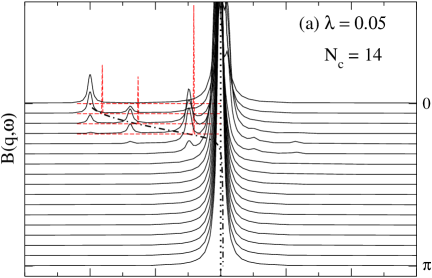
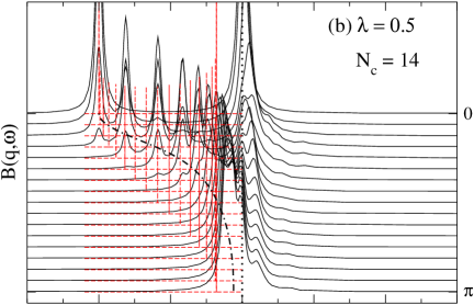
Figure 1: (colour online) Phonon spectral function $B(q,\omega)$ as obtained by the cluster approach, for $\alpha=0.4$ and different EP couplings $\lambda$ and cluster sizes $N_{\mathrm{c}}$. WC (a) and SC (b) – (d) analytical results (-  -  -  -, see text) have been multiplied by a factor of 10. Also shown are the bare phonon frequency $\omega_{0}$ (${\mathinner{\cdotp\cdotp\cdotp\cdotp\cdotp\cdotp}}$), and the polaron band dispersion $E_{q}-E_{0}$ (— $\cdot$ —) as calculated with the method of [37].

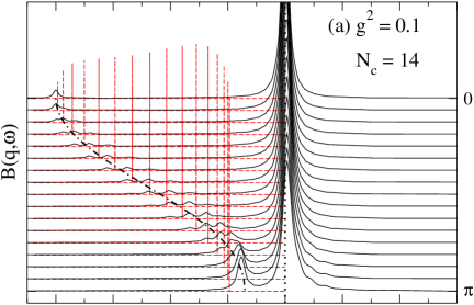
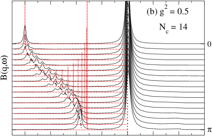
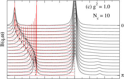
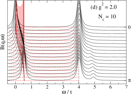
Figure 2: (colour online) As in figure 1, but for $\alpha=4$ and for different couplings $g^{2}$. WC (a) and SC (b) – (d) (-  -  -  -, see text) analytical results are shown on a logarithmic scale.

Similar to figure 1(c), figure 2(c) features a mirror image of the lowest polaron band—shifted by $\omega_{0}$—with extremely small spectral weight, which is barely visible for the number of Chebyshev moments—determining the energy resolution—used here.

In the non-adiabatic case, small polarons exist even at intermediate EP coupling (see [7] and references therein). Therefore, as underlined by the above comparison of the bandwidths, the SC approximation agrees well with the exact results even for $g<g_{\mathrm{c}}$ (figure 2(b)) and more than ever for $g=g_{\mathrm{c}}$ (figure 2(c)).

By contrast, for $\alpha=0.4$, a large-polaron state exists for $\lambda\approx\lambda_{\mathrm{c}}$, and both the WC (not shown) and the SC approximation fail to reproduce the characteristic IC features of figures 1(b) and 1(c).

Strong coupling:

In the SC limit, the low-energy part is separated from the phonon line for both the adiabatic and the anti-adiabatic case (figures 1(d) and 2(d)), and the full spectral function has the form given by equation (39). Moreover, the effect of the polaron band-narrowing is more pronounced for the adiabatic case, as the small-polaron band at fixed $\lambda$ has the half-width $\widetilde{W}=W\rme^{-2\lambda/\omega_{0}}$. In fact, there is no visible dispersion in the lower or upper band in figure 1(d). As expected, for these parameters, the SC approximation fits well the numerical results.

Another general feature related to the $\omega_{0}$-dependence of the spectral function becomes apparent if we compare the heights of peaks in figures 1 and 2 (the ordinate scale in figure 1 is about a factor of five larger than that in figure 2). This dependence reflects the fact that the transition probability at low temperatures is proportional to the density of polaron states in the coherent band. The latter quantity increases with decreasing bandwidth, and the pronounced difference between adiabatic and anti-adiabatic spectral functions in the SC limit is evident from equation (39), where the height of the peaks is dominated by the factor $1/\widetilde{W}\propto\rme^{2\lambda/\omega_{0}}$.

We conclude that the WC approximation based on the second-order electron spectral function, and the Hartree approximation for the SC small-polaron limit are able to grasp the main qualitative features of the phonon spectral function across the range of model parameters. However, as discussed in section 1, the numerical calculations do not represent exactly the limit of negligible charge-carrier concentration, owing to the restricted cluster volume. A direct comparison with results obtained by carrying out the limiting procedure for the analytical formulas in section 3.1 would be possible only for $N\to\infty$.

On the other hand, no restrictions concerning the charge carrier concentration were imposed in deducing equation (15) in section 3.1.1 and equation (37) in section 3.1.2. Consequently, the analysis of the latter equations outlined in section 3.1 permits us to discuss the additional features of spectra for non-negligible carrier concentrations revealed by the numerical results. First, the discussion in section 3.1.1 strongly suggests that the low-energy peaks of finite width correspond to the solutions of equations (19) – (23) at fixed wavevector $q$ if $\mu$ lies above the bottom of the electron (polaron) band. Second, at finite concentrations, the contributions of the incoherent part $A_{\mathrm{ic}}$ of the electron (polaron) spectral function to $\mathrm{Im}\,\Pi(q,\omega)$ are not negligible and, in this way, additional maxima above $\omega=\omega_{0}$ occurring in the numerical results may be understood as originating from phonon-assisted processes implied in $A_{\mathrm{ic}}$. Finally, the non-zero $\mathrm{Re}\,\Pi(q,\omega)$ in general causes a shift of the bare phonon line away from $\omega=\omega_{0}$ but, according to numerical results, the latter is not very pronounced in the WC and SC cases.

5 Summary

We have presented results for the phonon spectral function of the Holstein polaron in all relevant parameter regimes obtained by a reliable and systematic cluster approach similar to cluster perturbation theory. The characteristic features of the spectra have been discussed and successfully related to analytical self-energy calculations valid at weak and strong coupling, respectively. As far as a direct comparison is possible, our findings are in agreement with previous work on the phonon dynamics.

In particular, we have pointed out the important differences between weak, intermediate and strong coupling, on the one hand, and between the adiabatic and the anti-adiabatic regime, on the other hand. As revealed by the analytical results, the phonon spectra of the Holstein polaron are dominated by the bare, unrenormalized phonon line and the renormalized polaron band dispersion. At intermediate coupling, additional features such as level repulsion and mirror images of the polaron band have been observed. Together with previous studies of the electron spectral function and the renormalization of phonon energies, this work provides a fairly complete picture of the spectral properties of the one-dimensional Holstein polaron, which has been in the focus of intensive investigations over several decades due to the wide-spread relevance of polaron physics.

References

References

- [1] C. Hartinger et al., Phys. Rev. B 69, R100403 (2004).
- [2] C. Hartinger, F. Mayr, A. Loidl, and T. Kopp, Phys. Rev. B 73, 024408 (2006).
- [3] C. Battaglia et al., Phys. Rev. B 72, 195114 (2005).
- [4] T. Holstein, Ann. Phys. (N.Y.) 8, 325; 8, 343 (1959).
- [5] A. S. Alexandrov, Phys. Rev. B 46, 2838 (1992).
- [6] J. Tempere and J. T. Devreese, Phys. Rev. B 64, 104504 (2001).
- [7] M. Hohenadler et al., Phys. Rev. B 71, 245111 (2005).
- [8] S. Datta, A. Das, and S. Yarlagadda, Phys. Rev. B 71, 235118 (2005).
- [9] A. S. Alexandrov and N. Mott, Polaron & Bipolarons (World Scientific, Singapore, 1995).
- [10] H. Fehske, A. Alvermann, M. Hohenadler, and G. Wellein, in Polarons in Bulk Materials and Systems with Reduced Dimensionality, Proceedings of the International School of Physics “Enrico Fermi”, Course CLXI (North Holland, Amsterdam, in print).
- [11] S. Sykora et al., Phys. Rev. B 71, 045112 (2005).
- [12] S. Sykora, A. Hübsch, and K. W. Becker, cond-mat/0505687 (unpublished).
- [13] C. E. Creffield, G. Sangiovanni, and M. Capone, Eur. Phys. J. B 44, 175 (2005).
- [14] M. Hohenadler et al., cond-mat/0601673 (unpublished).
- [15] W. Q. Ning, H. Zhao, C. Q. Wu, and H. Q. Lin, Phys. Rev. Lett. 96, 156402 (2006).
- [16] S. Sykora, A. Hübsch, and K. W. Becker, cond-mat/0605463 (unpublished).
- [17] D. Meyer, A. C. Hewson, and R. Bulla, Phys. Rev. Lett. 89, 196401 (2002).
- [18] W. Koller, D. Meyer, and A. C. Hewson, Phys. Rev. B 70, 155103 (2004).
- [19] A. S. Alexandrov, V. V. Kabanov, and D. K. Ray, Phys. Rev. B 49, 9915 (1994).
- [20] O. S. Barišić, cond-mat/0602260 (unpublished).
- [21] S. Engelsberg and J. R. Schrieffer, Phys. Rev. 131, 993 (1963).
- [22] A. S. Alexandrov and J. R. Schrieffer, Phys. Rev. B 56, 13731 (1997).
- [23] D. Sénéchal, D. Perez, and M. Pioro-Ladrière, Phys. Rev. Lett. 84, 522 (2000).
- [24] D. Sénéchal, D. Perez, and D. Plouffe, Phys. Rev. B 66, 075129 (2002).
- [25] M. Hohenadler, M. Aichhorn, and W. von der Linden, Phys. Rev. B 68, 184304 (2003).
- [26] J. Loos, M. Hohenadler, and H. Fehske, J. Phys.: Condens. Matter 18, 2453 (2006).
- [27] L. P. Kadanoff and G. Baym, Quantum Statistical Mechanics (Benjamin-Cumming, Reading, MA, 1962).
- [28] V. L. Bonch-Bruevich and S. V. Tyablikov, The Green Function Method in Statistical Mechanics (North-Holland Publ. Co., Amsterdam, 1962).
- [29] H. Fehske, J. Loos, and G. Wellein, Z. Phys. B 104, 619 (1997).
- [30] H. Fehske, J. Loos, and G. Wellein, Phys. Rev. B 61, 8016 (2000).
- [31] G. D. Mahan, Many-Particle Physics, 2nd ed. (Plenum Press, New York, 1990).
- [32] D. N. Zubarev, Nonequilibrium statistical thermodynamics (Plenum Press, New York, 1974).
- [33] I. G. Lang and Y. A. Firsov, Zh. Eksp. Teor. Fiz. 43, 1843 (1962), [Sov. Phys. JETP 16, 1301 (1962)].
- [34] J. Schnakenberg, Z. Phys. 190, 209 (1966).
- [35] J. Loos, Z. Phys. B 96, 149 (1994).
- [36] A. Weiße, G. Wellein, A. Alvermann, and H. Fehske, Rev. Mod. Phys. 78, 275 (2006).
- [37] J. Bonča, S. A. Trugman, and I. Batistic, Phys. Rev. B 60, 1633 (1999).