Clustering instability in a freely falling granular jet

Abstract

This paper investigates a clustering instability of a freely falling granular jet composed of $100\mu\textnormal{m}$ glass spheres. The granular flow out of a circular nozzle starts out spatially uniform and then, further downstream, breaks up into well defined clusters. The role of air is investigated in this phenomenon by changing the ambient air pressure down to $1/5000^{\textnormal{th}}$ atm. An optical method is used that measures inhomogeneities in the flow in order to quantify the growth of the clusters. Clustering is observed down to the lowest pressure and the presence of air leads to larger drops but does not initiate the drop formation. The analysis shows that the drop size is set by fluctuations on the order of the size of the particles at the nozzle.

I I. Introduction

Granular media often appear to behave like ordinary fluids. One can pour sand into a bucket or use it in hour glasses. This paper investigates how a freely falling granular jet emanating from an aperture becomes inhomogeneous and starts to form droplets (Fig. 1) similar to an ordinary fluid column breaking up due to the Rayleigh-Plateau instability eggers . Despite this apparent similarity in behavior there are considerable differences between fluid and granular flows. The fluid jet instability is driven by the surface tension of the liquid. Dry, non-cohesive granular media, however, do not possess surface tension, so it is surprising to observe clustering in a granular jet.

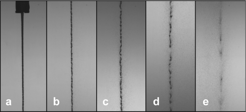
Figure 1: $100$ micron glass spheres draining from the $4$ mm wide circular nozzle at atmospheric pressure. This porous funnel is the same as used in the experiment. Pictures are taken at different depths $z$ below the nozzle. (a) at the nozzle; (b) $z=25$ cm; (c) $z=55$ cm; (d) $z=75$ cm; (e) $z=130$ cm.

Due to the lack of surface tension, the clustering instability must be driven by something else. In general, inhomogeneities in granular flows are quite common due to friction between particles and geometrical constraints imposed by boundaries. This can lead to arching and jamming. In the case studied here, however, the clusters form in the absence of boundaries. This distinguishes it from other clustering phenomena in granular flows such as density waves in funnels and vertical pipes baxter ; schick ; bertho ; raafat ; veje1 ; veje2 .

The clustering of freely falling granular jets appears to be generic. Recent experiments revealed that after the impact of a large sphere on a loosely packed bed of small particles a surprisingly tall granular jet emerges thoroddsen ; lohse ; royer . In this case as well the jet breaks up into droplets whose diameter is comparable to the jet diameter. This is another example of drop formation in the absence of nearby boundaries.

This study investigates, as a function of air pressure, drop formation from the flow out of a funnel. Air is important when dealing with small grains. Viscous drag can easily exceed the particle’s weight for the $100$ $\mu$m glass spheres used in this experiment. Moreover, investigating the role of air enables a comparison with recent experiments on drop formation in an underwater granular jet schaflinger ; nicolas . In my experiment I can tune the influence of the surrounding ”liquid” - namely the air. Studying the effect of air in this phenomenon is important for pinpointing the clustering mechanism. In particular, I study the properties of the drops, such as their size and growth as they freely fall, as a function of pressure.

The typical drop size decreases with decreasing pressure down to some threshold pressure below which the size remains unchanged. Thus, air influences the clustering but is not necessary for initiating the process. At all pressures the drops grow as they fall. The growth is well fit with a gravitational stretching function which indicates that perturbations of the order of a grain size at the nozzle serve as nucleation points for the drops. At higher pressures the jet atomizes below some depth. The depth at which disintegration occurs increases with decreasing pressure. At the lowest available pressure, $p\approx 1/5000^{\textnormal{th}}$ atm, the jet does not disintegrate within the experimentally accessible range of depth.

The following section gives an overview of inhomogeneities that can arise in granular flows. Section III describes the experimental method. The next section contains the experimental results and is followed by a discussion and conclusion in sections V and VI.

II II. Background

Intermittency and clogging are intrinsic features of granular flows. This is due to friction between grains and geometric constraints that prevent grains from flowing past each other when the flow is confined by boundaries (jamming). For finer particles air can also induce intermittency. This is observed in various systems, such as flow down a vertical pipe or in hourglasses schick ; bertho ; raafat ; wu ; veje1 ; veje2 . In my experiment the system undergoes a change from a dense granular funnel flow to a freely falling flow. Both regimes are susceptible to intermittency and clustering. In the following, different mechanisms that create inhomogeneities in granular flows and gases are reviewed.

II.1 A. Density waves

Density fluctuations can propagate through a flow, such as in vertical pipes schick ; bertho or funnel flow. Granular funnel flow and the related hopper flow have been extensively studied in the literature. The flow out of a nozzle can become inhomogeneous in a 2D as well as a 3D funnel system brown ; baxter . As the grains move downward under the influence of gravity, arches form near the nozzle that can temporarily hold up the flow before they collapse. The presence of these density waves is enhanced when the grains are rough and is suppressed when the grains are smooth spheres baxter .

II.2 B. Interstitial fluid effects

Apart from grain-grain and grain-boundary interactions, interstitial fluid such as air can profoundly affect the flow. This is especially important for systems such as mine where the particle size is well below $1$ mm duran . In this regime hydrodynamic forces can influence the dynamics strongly via viscous drag and pressure gradients building up inside the bed. The latter occurs because the movement of air is impeded inside a porous medium. In typical experimental settings ($v\lesssim 1$ m/s, $p=1$ atm) this effect does not matter much for grain sizes $\gtrsim 1$ mm, but becomes important for smaller media. As a result, the granular flow out of an aperture can become oscillatory wu ; veje1 ; veje2 . This so-called “ticking” is due to pressure gradients inside the bed that create a back-flow of air into the nozzle.

In cases where the interstitial fluid is a liquid, interesting flow instabilities have been observed nicolas ; schaflinger . Nicolas nicolas studied a system similar to mine, namely a granular jet emanating from a nozzle, but in the presence of a liquid. Depending on the grain and liquid parameters, the jet can either remain homogeneous or become unstable and form blobs similar to the clusters in my experiment. The origin of this instability still remains unclear. Nicolas showed that treating the suspension jet as a fluid with some effective viscosity cannot explain this instability.

II.3 C. Inelastic Clustering

A granular gas is dissipative due to the inelastic nature of the collisions between the grains. Therefore, without external energy supply the gas cools down with time and eventually freezes mcnamara ; goldhirsch ; poeschel . However, it does not cool homogeneously, but forms clusters. When a fluctuation increases the density locally, the collision rate goes up in this region. Due to the increased dissipation, the granular temperature decreases which in turn lowers the pressure. The resulting pressure gradient will enhance migration of particles into that region, thereby increasing the density even further. Eventually, these regions grow into clusters.

II.4 D. Cohesion

Humidity in the air and surface charges can induce cohesive forces between particles duran . Condensates from ambient humidity create liquid bridges causing particles to stick together. As with interstitial fluid effects, the influence of cohesion depends strongly on the size and the density of the particles. Smaller and lighter media are more susceptible to cohesive forces. Cohesion does not cause intermittency per se, but can dramatically change the rheological properties of granular media. In extreme cases it leads to clumping and caking. These effects can be controlled but not completely eliminated. In this experiment, I keep the relative humidity at $50\%$, which provides enough ions to eliminate surface charges, but does not result in clumping. However, small residual cohesive forces could potentially induce clustering in the freely falling jet.

III III. Experimental Method

In this paper I exclusively study $d=100$ $\mu\textnormal{m}$ spherical glass beads (Mo-Sci Corp., $\rho=2500$ g/l) (Fig. 1). In order to investigate the clustering in the emerging jet quantitatively, an optical system was set up to measure inhomogeneities in the jet - similar to ones used in previous studies for measuring intermittent granular flows in hourglasses and vertical pipes schick ; raafat ; veje1 . The basic idea is to measure the light intensity of a laser shining through the falling grains. The fluctuations in the intensity allow me to record inhomogeneities in the flow. This method does not measure density variations, but rather the emergence of undulations on the jet surface and gaps.

The schematics of the setup are shown in Fig. 2. The funnel is mounted inside and near the top of a $14$ cm wide acrylic tube whose diameter is large enough so that the particles are always far from the wall. A $9$ cm wide cylindrical reservoir feeds the grains into a porous tube. At the bottom of this tube a disc with a $4$ mm circular aperture is attached from which the particles emerge and then freely fall down the tube. There is a remote controlled shutter beneath the nozzle to initiate and stop the flow. The pressure inside the acrylic tube can be pumped down to $0.02$ kPa. For air, this corresponds to a mean free path of $0.3$ mm ($\approx 3$ d) chemistry . The pressure is monitored with a pressure gauge mounted on the lid (Granville-Phillips, Convectron gauge 375). An oil filter (K.J. Lesker micromaze foreline trap) and a shut-off valve was installed between the system and the vacuum pump to avoid contamination of the system with oil vapor that might emanate from the vacuum pump.

A prerequisite for this experiment is to ensure a steady non-changing flow out of the nozzle. It is known that air pressure gradients across the bed can cause oscillatory flow (”ticking”) out of the nozzle wu . Even equalizing the pressure in the reservoir with the pressure at the nozzle is not sufficient for steady flow conditions. To eliminate ticking, I made the tube coming from the reservoir porous. It is made out of metal mesh ($0.0014^{\prime\prime}$ wire mesh $325$x$325$) that is permeable to air, but not to the particles, thereby allowing pressure equalization through the boundaries (Fig. 3). This ensures a stable flow rate at all pressures (Fig. 4).

The whole optical system is mounted on a platform that is moveable in the vertical direction and can be lowered to $2.1$ m below the nozzle. Since the width of the freely falling particle flow exceeds the diameter of the laser beam (5 mW laser diodes from z-bolt.com), the light is spread out to a sheet to capture the entire horizontal spread of the flow. This is achieved by shining the light through a $8$ mm diameter glass rod. The beam is also focused in the horizontal plane by a lens to ensure that the beam waist is smaller than the emerging structures. The vertical width is $0.3$ mm ($\approx 3d$). After the laser sheet passes through the particle flow, it is refocused by a cylindrical lens onto a photodiode (Silonex SLD-68HL1D) that measures the intensity. A current amp is used to convert the diode current, which is linearly proportional to the incident light intensity, into a voltage signal. The signal is inverted since the quantity of interest is the amount of light that is screened by the jet. We refer to this signal as the blockage $B$. The frequency response is flat up to at least $100$ kHz. The signal is recorded with an A/D converter card at a sampling rate of $48$ kHz. The baseline of the signal changes with vertical position due to imperfections of the acrylic tube. The signal is scaled with the baseline at each position before each experimental run.

In order to convert time scales into length scales, the local average velocity of the flow is measured by cross-correlating the intensity signal of two closely spaced laser sheets (vertical distance$=5.1$ mm). In order to avoid cross-talk between the two photodiodes through scattered light a shutter is mounted near the cylindrical lens. A $2$-channel spectrum analyzer (SRS SR780) obtains the cross correlation between the two signals in real time.

When calculating autocorrelations, the mean of the signal is subtracted and the autocorrelation is normalized to $1$ at zero time delay $\Delta t$. In that way, the autocorrelation approaches zero at large $\Delta t$. Near the nozzle, the signal to noise is low and a noise floor appears in the autocorrelation. The electric noise floor is measured directly by obtaining the autocorrelation of the laser signal without the granular jet. It is then subtracted from the autocorrelation.

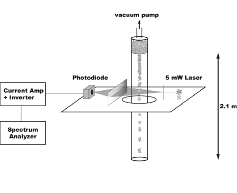
Figure 2: Setup. The granular jet emerges from the reservoir at the top of the $14$ cm wide acrylic tube. The tube is connected to a vacuum pump and the pressure is measured with a pressure gauge mounted on the lid. The optical platform can be adjusted to any height between the nozzle and $2.1$ m below. The light from a $5$ mW ($\lambda=650$ nm) laser diode is focused by a lens, then passed through a glass rod to spread it out and finally refocussed with a cylindrical lens onto a photodiode. An identical laser sheet (not shown) is mounted $5.1$ mm below the first sheet. The signals of the two photodiodes are passed to two current amps that also invert the signals. The two signals are cross-correlated with a spectrum analyzer and one of them is sent to an A/D converter card.

Cohesion between particles is caused by liquid bridges and/or electrostatic interaction due to charge buildup duran . The latter is especially significant in dry atmospheres. To ensure stable conditions the laboratory is controlled at $50\%$ relative humidity. Moreover, the walls of the reservoir are grounded to avoid build up of charge through friction. After each run, the beads are exposed to ionized air to neutralize any charges that might have built up during the run.

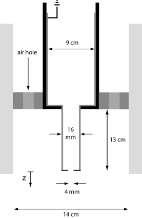
Figure 3: Schematics of the reservoir. The reservoir consists of a $9$ cm wide acrylic tube which feeds a $16$ mm wide porous tube. At the bottom of the porous tube I attached a metal disc with a $4$ mm circular aperture. The inside is covered with metal mesh and is grounded. The reservoir sits on a ring that has several holes in it to allow for pressure equalization between the reservoir and the lower part of the tube. The depth $z$ is measured from the nozzle.

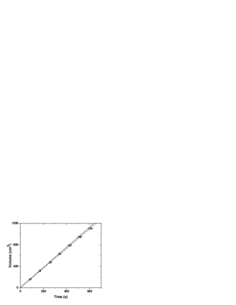
Figure 4: Volume flow vs. time. The solid and dashed lines are linear fits with respective slopes of $1.87$ and $1.82$ $\textnormal{cm}^{3}/\textnormal{s}$. $(\blacksquare)$, $p=101$ kPa; $(\blacktriangleright)$, $p=62$ kPa; $(\blacktriangle)$, $p=26$ kPa; $(\triangledown)$, $p=3$ kPa; $(\lozenge)$, $p=0.04$ kPa.

IV IV. Results

In order to compare the clustering at different pressures we need to know the flow rate out of the nozzle and the velocity of the jet as a function of pressure. As mentioned above, a porous tube is used to ensure steady flow at higher pressures. Furthermore, care has been taken to prepare the glass spheres in the reservoir in the same way after each run so that the packing fraction remains constant. Figure 4 shows the volume flow rate at different pressures. This was measured by recording how long it takes for the full reservoir to drain $158$ $\textnormal{cm}^{3}/\textnormal{s}$ at a time. I do not let the reservoir empty completely, since the flow rate changes when the fill height is low. The flow rate is nearly constant for all pressures: At atmospheric pressures the flow rate is $1.82$ $\textnormal{cm}^{3}/\textnormal{s}$, which is slightly lower than at $p=0.04$ kPa, where it is $1.87$ $\textnormal{cm}^{3}/\textnormal{s}$. This few percent difference is negligible for the subsequent analysis. The constant flow rate allows a direct comparison of the clustering at different pressures.

In order to convert the signals recorded in the time domain into the length domain, we need to know the velocity at each height. Figure 5 shows the velocity of the jet versus depth at four pressures. In the absence of any hydrodynamic drag force the velocity $v$ should just follow $v=\sqrt{2gz+v_{0}^{2}}$, where $z$ is the distance as measured from the aperture, $v_{0}$ the velocity at the nozzle and $g$ is the acceleration of gravity. When $(v^{2}-v_{0}^{2})/2$ is plotted against the depth $z$, the resulting curve is linear for simple free fall with a slope equal to the acceleration $a=g$. $v_{0}$ is constant within a few percent at all pressures. This is consistent with the constant flow rate found earlier. Down to the lowest available pressure we find a linear relationship between $(v^{2}-v_{0}^{2})/2$ and $z$ with a slope close to or equal to $g$. At higher pressures deviations are observed when the jet starts to disintegrate into a cloud of particles (Fig. 1 (e)). When $p=101$ kPa ($=1$ atm), this happens around $1.2$ m below the nozzle (Fig. 5 (d)). At this point the mean velocity stops growing with depth and the previously sharp cross-correlation peak becomes broad. When the pressure is lowered, the disintegration starts further downstream (Fig. 5 (c)). At the lowest pressure (Fig. 5 (a)), no disintegration is observed in the experimentally available range of depth.

The low drag on the jet at $p=101$ kPa is surprising given that the viscous drag on a single grain is substantial and would lead to a terminal velocity of $0.76$ m/s according to the Stokes formula for viscous drag on a sphere: $F_{\textnormal{Stokes}}=3\pi\mu dv$. A possible explanation is that the air is essentially trapped inside the jet so that it appears solid. Treating the jet as a porous medium, one can estimate the time it takes for air to penetrate the jet. Inside a porous medium, the pressure obeys a diffusion equation carman . The diffusion constant is $D=(P_{0}k)/(\mu(1-\phi))$, where $P_{0}$ is the ambient gas pressure, $\mu$ the dynamic viscosity of air, and $k$ the permeability of the granular medium at a packing fraction $\phi$. The permeability is an empirical constant that is well approximated by the Carman-Kozeny relation carman : $k=d^{2}(1-\phi)^{3}/(180\phi^{2})$. The value for $D$ is $0.3$ $\textnormal{m}^{2}/\textnormal{s}$ after substituting numerical values for the constants: $\mu=1.8\cdot 10^{-5}$ Pa s, $P_{0}=101$ kPa and $\phi=0.5$. The latter is a typical packing fraction for a random loose pack of spheres. This value decreases as the jet falls and gets stretched. The typical time $\tau$ for air to diffuse into the jet is therefore $\tau\approx r_{jet}^{2}/(2D)=6.7$ $\mu\textnormal{s}$. This is small compared to other typical timescales of the system, such as the time it takes for a grain to fall its own diameter: $d/v\approx 10^{-4}$ s. This means that the jet is permeable to air. Therefore, a more sophisticated hydrodynamic description is needed to explain the low drag on the jet at atmospheric pressure.

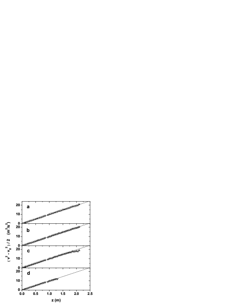
Figure 5: Velocity profile of jet at different pressures. In all panels, $v_{0}=0.36$ m/s. The solid lines are linear fits to the data. The slope represents the acceleration $a$. (a) $p=0.027$ kPa, $a=9.8$ m/s; (b) $p=0.67kPa$, $a=9.8$ m/s;(c) $p=49$ kPa, $a=9.8$ m/s;(d) $p=101$ kPa, $a=9.7$ m/s.

Figures 6 and 7 display typical time traces of the signal at $p=0.027$ kPa and atmospheric pressure, respectively. Just below the nozzle, $z=2$ cm, drops have not yet formed and the signal fluctuates only slightly. At $z=50$ cm the fluctuations have visibly increased and finally, at $z=150$ cm, the signal contains clear peaks which show the presence of well defined drops.

Figure 6: Blockage at different depths, $z$, at $p=0.027$ kPa. The length of the arrow equals the dip position of the corresponding autocorrelation.

At atmospheric pressure the behavior is similar. Comparing the time traces at $z=50$ cm, it is apparent that the drops are bigger at atmospheric pressure. In atmosphere only depths up to $\approx 120$ cm can be probed, since the jet disintegrates beyond that depth.

Figure 7: Blockage at different depths, $z$, at $p=101$ kPa. The length of the arrow equals the dip position of the corresponding autocorrelation.

In order to illustrate the evolution of the drops, the fluctuations of the blockage signal as a function of depth have been plotted (Fig. 8). The fluctuations are just the standard deviation, $\Delta B$, divided by the mean of the signal $<B>$. In vacuum (Fig. 8 (a)) the fluctuations increase monotonically with depth and then saturate. Similarly, at atmospheric pressure the fluctuations increase, but then slowly decrease (Fig. 8 (b)).

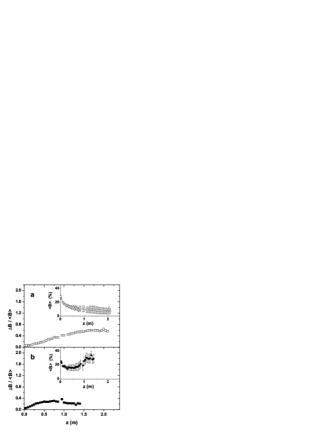
Figure 8: Blockage fluctuations as a function of depth. (a) $p=0.027$ kPa, (b) $p=101$ kPa. Insets: Mean and standard deviation of the blockage as a function of depth at the respective pressure. The error bar delineates the standard deviation $\Delta B$.

The insets in Fig. 8 show how $<B>$ and $\Delta B$ vary with depth. At low pressure, the mean decreases with depth while the standard deviation increases. This reflects the increase of undulations and gaps with increasing depth. At atmospheric pressure (Fig. 8 (b)), the mean varies non-monotonically. Beyond $1$ m it even exceeds the value at small depth when the jet is still compact. The standard deviation, however, stops increasing far away from the nozzle.

The reason for this marked difference in behavior is that in the presence of air, the jet does not stay collimated far away from the nozzle as it does at low pressures. This leads to an increased blockage as the jet starts to spread. Furthermore, there is more spray, presumably caused by advection of particles by the surrounding air. The optical signal is sensitive to this spray since it scatters the light. This explains why the mean blockage starts to rise again below $60$ cm or so. It should also be noted that even if the jet is still homogeneous, the blockage does not reach $100\%$ at both pressures, since the laser sheet is wider than the jet diameter.

One way to analyze the signal is to choose a threshold and convert the blockage signal into a binary sequence as done by Raafat and coworkers raafat . Anything above the threshold is considered a drop, anything below a gap. The resulting histogram for my experiment is shown in Fig.9. This was obtained at $p=0.027$ kPa for two heights and the threshold was taken to be the signal average. The drop histogram displays a clear peak at $z=150$ cm, while it is less pronounced at $z=50$ cm. The gap histogram remains flat and falls off at large gap sizes in both cases. The high occurrence of very small drop and gap sizes is due to electronic noise and particle spray. The histograms bear some resemblance to the ones in the vertical pipe flow studied by Raafat et al. raafat . Fig. 9 shows the emergence of a typical drop size, while the gap size distribution is broad.

This analysis is prone to noise. The peak in the drop histogram appears only below $50$ cm, even though inhomogeneities appear earlier (by visual inspection with a stroboscope). A more sensitive analysis is the autocorrelation as shown in Fig.10.

Figure 9: Histogram of drops and gaps at $p=0.027$ kPa. In both panels the solid line corresponds to $z=150$ cm and the dashed line to $z=50$ cm. The threshold to discriminate between drop and gaps is the average of the signal. (a) drop histogram; (b) gap histogram

Autocorrelations are displayed for two different pressures. At both pressures, a dip and a peak in the autocorrelation develops, though the peak is far less pronounced at $p=101$ kPa. The dip position does not change with depth at $p=0.027$ kPa. At atmospheric pressure, the dip remains constant as a function of depth initially, but then moves to higher $\Delta t$ below $z=80$ cm. Also, the dip position at $p=101$ kPa is significantly larger than at low pressure. At low depths ($z<80$ cm) it is $7.0\cdot 10^{4}$ s compared to $3.8\cdot 10^{-4}$ s at $p=0.027$ kPa.

A priori it is not clear whether the dip represents the time scale of drops or gaps. Looking at the time traces in Figs. 6 and 7, drops and gaps have similar sizes. The histogram (Fig. 9) confirms this observation. The drop and gap size distribution are both broad and fall off around $0.008$ s. Therefore, the dip reflects the typical size of the fluctuations in the time domain. The length of the arrows in Figs. 6 and 7 represent the dips in the respective autocorrelations of the time traces. They show good agreement with the typical fluctuation size by visual inspection.

Summarizing the above, we identify the dip position with the typical fluctuation size (in the time domain) and find that with increasing depth it stays constant for low pressures and becomes larger for atmospheric pressure. It follows that the clusters and gaps continually grow as they are stretched by the increasing velocity as a function of depth.

Figure 10: Autocorrelation at different heights. Left panels show data at $p=0.027$ kPa, the right panels at $p=101$ kPa. The depth at which the signal was recorded is indicated in each panel. The insets in the upper panels show all the autocorrelations for the respective pressure.

In order to understand the growth of the drops it is instructive to consider the case where the jet is just stretched due to gravity ignoring all other interactions. The equations of motion for two grains, one right at the nozzle starting with velocity $v_{0}$, the other a distance $\lambda_{0}$ below, are respectively:

$$z = v_{0}t+\frac{1}{2}gt^{2}$$ (1)

$$z^{\prime} = \lambda_{0}+v_{1}t+\frac{1}{2}gt^{2}$$ (2)

where $v_{1}=\sqrt{2g\lambda_{0}+v_{0}^{2}}$ is the velocity the grain attains by falling a distance $\lambda_{0}$. Due to gravitational acceleration the initial grain separation $\lambda_{0}$ will grow in time as $\lambda(t)=z^{\prime}-z$.

Parameterizing $t$ with $z$ we obtain

$$\lambda(z)=\lambda_{0}+\frac{v_{0}^{2}}{g}\left(\sqrt{\frac{2g\lambda_{0}}{v_{0}^{2}}+1}-1\right)\left(\sqrt{\frac{2gz}{v_{0}^{2}}+1}-1\right).$$ (3)

When $\lambda_{0}\ll\frac{v_{0}^{2}}{2g}$ this reduces to

$$\lambda(z)=\lambda_{0}\sqrt{\frac{2gz}{v_{0}^{2}}+1}.$$ (4)

Far away from the nozzle, when $z\gg\frac{v_{0}^{2}}{2g}$, this can be further simplified to

$$\lambda(z)=\lambda_{0}\frac{\sqrt{2gz}}{v_{0}}.$$ (5)

Since $\sqrt{2gz}$ is just the velocity $v(z)$ at depth $z$ for $z\gg\frac{v_{0}^{2}}{2g}$, equation 5 can be written as

$$\frac{\lambda_{0}}{v_{0}}=\frac{\lambda(z)}{v(z)}\equiv T,$$ (6)

where $T$ is the time it takes to fall a distance $\lambda(z)$ at depth $z$. This time is constant for $z\gg\frac{v_{0}^{2}}{2g}$. We can now compare $T$ with the dip position of the autocorrelation which is a measure of how long it takes for a drop to fall. At $p=0.027$, the dip position is constant at all depths to within a few percent: $3.8\cdot 10^{-4}$ s; the clusters just get stretched by falling in gravity. The velocity at the nozzle is $v_{0}=0.36$ m/s. Therefore, $\lambda_{0}=1.4\cdot 10^{-4}\textnormal{m}=1.4d$ (this also justifies the approximation $\lambda_{0}\ll\frac{v_{0}^{2}}{2g}$ to simplify equation 3). At atmospheric pressure the dip position is larger and grows below $z=80$ cm. Using the value of the dip position for smaller depths, we find $\lambda_{0}=2.5\cdot 10^{-4}\textnormal{m}=2.5d$.

In order to see how the drop growth compares with pure gravitational stretching, I plot the dip length as a function of depth measured at four different pressures (Fig.11). The dip positions have been converted into length scales by multiplying each of them with the local velocity that is obtained from Fig. 5. I plot the gravitational stretch equation (eqn. 3) for each data set using the value for $\lambda_{0}$ we found from our previous considerations, so there are no free fitting parameters. The dip lengths have been rescaled with the particle diameter. At $p=0.027$ kPa, the data is well fit by this equation. Unfortunately, the optical setup is not sensitive enough to pick up inhomogeneities above $10$ cm depth. The fit for higher pressures agrees with the data until the onset of atomization. At that point, the dip position grows larger than it would just with gravitational stretching.

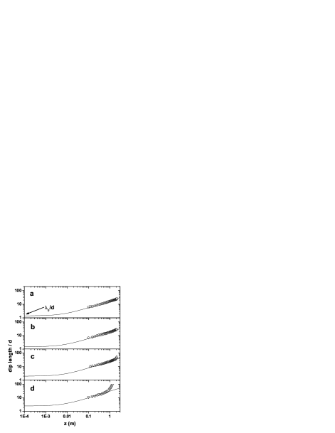
Figure 11: Dip length vs. depth at different pressures. Each dip position has been converted into a length scale by multiplying it with the local velocity. The solid lines are fits from equation 3. The error bars are the size of the symbols. (a) $p=0.027$ kPa; (b) $p=0.67kPa$; (c) $p=49$ kPa; (d) $p=101$ kPa.

In Fig. 12 I track the dip position in the autocorrelation as a function of pressure at constant depth $z=20$ cm below the nozzle. The dip position decreases with decreasing pressure until about $p\approx 0.1$ kPa at which it stays constant down to the lowest available pressure $0.02$ kPa. As we have seen before, the air has an appreciable effect on the drop size. The dip changes by almost a factor of two. Moreover, it shows that air has no effect below $0.1$ kPa. Below that pressure the dip position remains constant over one order of magnitude in pressure.

Figure 12: Dip position as a function of pressure at $z=20$ cm.

V V.Discussion

I have shown that the clustering of a freely falling granular jet is influenced by the presence of air, but occurs even at low pressures. At the lowest available pressure, $p=0.02$ kPa, the mean free path exceeds the particle size by a factor of $3$, so air effects should be negligible. Moreover, at constant depth, the position of the first dip in the autocorrelation function, which is a measure of the typical size of the structure, stays constant below $0.1$ kPa down to $0.02$ kPa (Fig.12). Therefore, air-grain interactions can be ruled out as the initial cause of the clustering.

It is worth noting that other granular phenomena that depend on the ambient pressure lose their pressure dependence below $\approx 0.1$ kPa. Granular size separation in vibrated beds depends strongly on pressure when the grain size is small ($d\lesssim 500\mu$m)mobius ; king . It has been found that below $0.1$ kPa air ceases to play a role. Another granular phenomenon that depends on air is heaping. The surface of a bed of small particles ($d\lesssim 600\mu\textnormal{m}$) starts to tilt when vertically vibrated pak . It was found that heaping dramatically decreases below $1$ kPa, since the mean free path of air becomes comparable to the grain size. This suggests that it is for this same reason that the dip position stops changing at low pressures in Fig.12.

This experiment does not measure density, so I cannot distinguish between cluster growth through agglomeration and the stretching of a cluster due to gravity. Nevertheless, the latter is always present, so it is sensible to compare the growth in cluster size with gravitational stretching.

My results indicate that the instability arises from fluctuations on the granular level at the nozzle. At the lowest available vacuum, where air effects are negligible, gravitation is the only external force acting on the particles. Indeed, the fit for gravitational stretching is good at these low pressures. Extrapolating the drop growth back to the nozzle, I find the initial size to be of the order of a grain diameter.

At higher pressures deviations from the gravitational stretching are observed. The extrapolation yields an initial size that is almost a factor of two larger than at low pressures. Moreover, the jet starts to disintegrate into a cloud below some depth. This is presumably due to hydrodynamic interactions, since we do not observe this at low pressures, at least in the observable range of depths.

I did not observe clustering for grain sizes larger than $200\mu\textnormal{m}$. Visual inspection by strobing granular jets of larger particles did not reveal any inhomogeneities visible by eye. Smaller grains, on the other hand, give rise to strong clustering.

It is still unclear how these grain-sized fluctuations grow into drops of several particles. The fact that clustering is not observed for glass spheres $\gtrsim 200\mu\textnormal{m}$ suggests that cohesive forces might be responsible. However, if cohesive forces were dominant, so that the particles just stick together, the drops should not grow and remain constant in size once they are formed. On the other hand, the velocity correlations induced by inelastic collisions of equal particles do not depend on the mass of the particles and therefore should not depend on their size. They just depend on the coefficient of restitution. However, there are indications luding ; labous that the coefficient of restitution is size dependent. Experimentally labous and theoretically luding it was shown that smaller spheres give rise to a smaller coefficient of restitution. Therefore, a granular gas of small spheres should form clusters more rapidly than larger ones. Since I do not have any information on the coefficient of restitution of the glass spheres used in my experiment, it is unclear whether this size dependence could explain the absence of clusters in granular jets of large particles.

Regardless of the clustering mechanism, an initial perturbation is required that acts as a seed for the cluster. Since gravity cannot initiate fluctuations and air-grain interactions have been ruled out, this perturbation is likely to come from the nozzle. This is consistent with the finding that the cluster size extrapolates to a few grain diameters at the nozzle, which is a typical fluctuation in granular flows.

VI VI. Conclusion

In contrast to ordinary fluids, granular flows lack surface tension and are discrete in nature. Despite these fundamental differences, a freely falling jet becomes unstable and forms drops in both cases. However, the physical origin of the instability in the granular case is quite different from its fluid counterpart.

The length scale, after tracing it back to the nozzle using the gravitational stretch equation, turns out to be of the order of a grain size at all pressures. This suggests that granular fluctuations at the nozzle set the cluster size. Moreover, I have shown that the surrounding liquid, in my case air, is not required for drop formation. It does however, change the length scales by almost a factor of $2$ and ultimately leads to the atomization of the jet. The latter is not observed at low pressures.

These results might have implications on the clustering phenomenon found in suspensions nicolas ; schaflinger . They have typically been ascribed to an effective surface tension between the fluid and the sediment. My results show that fluctuations on the granular level can propagate downstream and thereby impose a length scale. This suggests that the granular nature of the sediment cannot be ignored and a continuous medium description is inadequate to explain this phenomenon.

This study also leaves some open questions: Clustering is not observed for glass spheres larger than $200\mu$m. This observation should give insight into the clustering mechanism which still remains unclear. How do fluctuations of single grains grow into clusters of many particles? Further studies are needed to answer this question.

The clustering of a freely falling granular jet is a novel granular instability that is initiated by fluctuations at the nozzle that are of the order of a grain diameter. These fluctuations grow into clusters downstream. The detailed structure of the drops may reveal information about these fluctuations that are experimentally difficult to access otherwise.

VII Acknowledgements

I thank H. Jaeger and S. Nagel for their support and guidance. I am grateful to X. Cheng, E. Corwin, M. Holum and J. Royer for useful discussions and suggestions. H. Krebs’s expertise was invaluable to build the apparatus. This work is supported by MRSEC, No. DMR-0213745.

References

- (1) J. Eggers, Rev. of Mod. Phys. 69, 865 (1997).
- (2) G.W. Baxter, R. P. Behringer, T. Fagert, and G.A. Johnson, Phys. Rev. Lett. 62, 2825 (1989).
- (3) K. Schick and A. Verveen, Nature 251, 599 (1974).
- (4) Y. Bertho et al., J. Fluid. Mech. 459, 317 (2002).
- (5) T. Raafat, J.P. Hulin, and H.J. Herrmann, Phys. Rev. E 53, 4345 (1996).
- (6) C. Veje and P. Dimon, Gran. Matt. 3, 151 (2001).
- (7) C.T. Veje and P. Dimon, Phys. Rev. E 56, 4376 (1997).
- (8) S. Thoroddsen and A. Shen, Phys. Fluids 13, 4 (2001).
- (9) D. Lohse et al., Phys. Rev. Lett. 93, 198003 (2004).
- (10) J. Royer et al., Nature Phys. 1, 164 (2005).
- (11) U. Schaflinger and G. Machu, Chem Eng. Tech. 22, 617 (1999).
- (12) M. Nicolas, Phys. Fluids. 14, 3570 (2002).
- (13) X.-l. Wu, K.J. Måløy, A. Hansen, M. Ammi, and D. Bideau, Phys. Rev. Lett. 71, 1363 (1993).
- (14) R. Brown and J. Richards, Trans. Instn. Chem. Engrs. 38, 243 (1960).
- (15) J. Duran, Sands, Powders and grains (Springer, 2000).
- (16) S. McNamara and W. Young, Phys. Fluids A 5, 34 (1993).
- (17) I. Goldhirsch and G. Zanetti, Phys. Rev. Lett. 70, 1619 (1993).
- (18) N.V. Brilliantov and T. Pöschel, Kinetic Theory of granular gases (Oxford University Press, 2004).
- (19) edited by D.R. Lide, Handbook of Chemistry and Physics (CRC Press, 1997).
- (20) P. Carman, Flow of gases through porous media (Butterworth Scientific, London, 1956).
- (21) M.E. Möbius, X. Cheng, G.S. Karczmar, S.R. Nagel, and H.M. Jaeger, Phys. Rev. Lett. 93, 198001 (2004).
- (22) N. Burtally, P.J. King, and M.R. Swift, Science 295, 1877 (2002).
- (23) H.K. Pak, E. van Doorn, and R.P. Behringer, Phys. Rev. Lett. 74, 4643 (1995).
- (24) L. Labous, A.D. Rosato, and R.N. Dave, Phys. Rev. E 56, 5717 (1997).
- (25) S. Luding, Ph.D. thesis, Universität Freiburg (1994).