Random Networks Tossing Biased Coins

Abstract

In statistical mechanical investigations on complex networks, it is useful to employ random graphs ensembles as null models, to compare with experimental realizations. Motivated by transcription networks, we present here a simple way to generate an ensemble of random directed graphs with, asymptotically, scale-free outdegree and compact indegree. Entries in each row of the adjacency matrix are set to be zero or one according to the toss of a biased coin, with a chosen probability distribution for the biases. This defines a quick and simple algorithm, which yields good results already for graphs of size $n\sim 100$. Perhaps more importantly, many of the relevant observables are accessible analytically, improving upon previous estimates for similar graphs. The technique is easily generalizable to different kinds of graphs.

I Introduction.

In our investigation concerning transcription networks, we came across a simple and effective way to generate a random ensemble of directed graphs having similar features as the experimental ones. Transcription networks are directed graphs that represent regulatory interactions between genes. Specifically, the link $a\rightarrow b$ exists if the protein coded by gene $a$ affects the transcription of gene $b$ in mRNA form by binding along DNA in a site upstream of its coding region BLA+04 . For a few organisms, such as E. coli and S. cerevisiae, a significant fraction of the wiring diagram of this network is known LRR+02 ; GBB+02 ; SSG+01 ; HGL+04 . The hope is to study these graphs, together with the available information on the genes and the physics/chemistry of their interactions, to infer information on the large-scale architecture and evolution of gene regulation in living systems. In this program, the simplest approach to take is to study the topology of the interaction networks. For instance, order parameters such as the connectivity and the clustering coefficient have been considered GBB+02 .

To assess a topological feature of a network, one typically generates so called “randomized counterparts” of the original data set as a null model. That is, an ensemble of random networks which bare some resemblance to the original. The idea behind it is to establish when and to what extent the observed biological topology, and thus loosely the living system under exam, deviates from the “typical case” statistics of the null ensemble. For example, a topological feature that has lead to relevant biological findings, in particular for transcription, is the occurrence of small subgraphs - or “network motifs” MSI+02 ; MIK+04 ; MBV05 ; WA03 ; YSK+04 . The choice of what feature to conserve (or not) in the randomized counterpart is quite delicate and depends on specific considerations on the system IMK+03 . The null ensemble used to discover motifs usually conserves the degree sequences of the original network, that is, the number of regulators and targets of each node. The observed degree sequences for the known transcription networks follow a scale-free distribution for the outdegree, with exponent between one and two, while being Poissonian in the indegree GBB+02 ; CLB05 . Motifs are then interpreted as elementary circuit-like building blocks and have been shown in many cases to work independently MA03 .

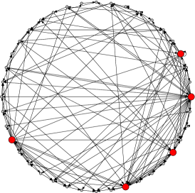
Figure 1: Example of a graph generated with our algorithm with $n=40,\ \beta=2.8,\ \alpha=1$. Nodes with more than ten outgoing edges are larger (red online).

In connection with this line of research, it is interesting to study random ensembles of graphs with probability distributions for the degree sequences that are similar to those observed experimentally, with the objective of characterizing theoretically some relevant topological observables, such as the subgraph distributions IMK+03 ; BB03 . Here, we describe a simple, and fast, algorithm that performs this task by tossing coins with prescribed random biases. Differently from more sophisticated techniques available in the literature IMK+03 ; RJB96 ; CDH+05 ; MKI+03 ; MR95 , our method is not designed to conserve a degree sequence, but rather as a general random graph model, that, in particular, can be used to generate graphs with degree distributions that agree with the observed power-law distributed outdegrees and compact indegrees IMK+03 . To this aim, the ensemble will be generated by a parametric model, where the adjustable parameters can be used for fits of real data-sets. Note that, with the weaker constraint on the degree distribution that we have chosen, it would be very inconvenient to generate the ensemble throwing degree sequences a priori from the given distributions and then using an algorithm designed for fixed degree sequences, which is necessarily more costly. We will see that, because of the extreme simplicity of our formulation, some observables can be computed analytically rather than estimated as in ref. IMK+03 . After introducing the algorithm and showing that the ensemble has the required features, we will compute the number of some observables that are relevant for transcription, such as triangular subgraphs.

II Algorithm.

Any directed graph $G_{n}$ with $n$ nodes is completely described by its adjacency matrix $A(G_{n})=[x^{(n)}_{i,j}]_{i,j=1,\dots,n}$, where $x^{(n)}_{i,j}=1$ if there is a directed edge $i\rightarrow j$, $0$ otherwise. Instead of square matrices, one may also consider rectangular matrices with a prescription on the scaling of the rows with the columns. In what follows we will deal with rectangular matrices $m_{n}\times n$ with $m_{n}\leq n$. As we will see, this is particularly useful for networks with power-law degree distributions having exponent equal or lower than two (for which the average diverges), to keep the asymptotics well-behaved. In the context of transcription networks, the hypothesis of rectangularity is well-motivated by the fact that typically only a subset of $m_{n}$ nodes encode for transcription factors (namely, they have outgoing edges). Thus, in a $m_{n}\times n$ matrix, the first $m_{n}$ columns will contain the incoming links to the transcription factors, and the next $n-m_{n}$ columns will correspond to non transcription-factor encoding genes. Note that in general nodes that send out edges are also receiving edges (Fig 2).

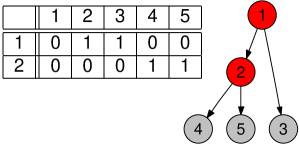
Figure 2: Example of a rectangular matrix and its associated graph. Nodes 1 and 2 represent transcription factors, and can regulate any other node. Nodes 3 to 5 are targets and only receive incoming links. In this case $m_{n}=2/5n$.

Our model ensemble can be defined by the following generative algorithm. For each row of $A$, (i) throw a bias $\theta$ from a prescribed probability distribution $\pi_{n}$ (ii) set the row elements of $A$ to be $0$ or $1$ according to the toss of a coin with bias $\theta$. Since each row is thrown independently, the resulting probability law is

$$\begin{array}[]{l}P\{x_{i,j}^{(n)}=e_{i,j},\,i=1,\dots,m_{n},j=1,\dots,n\}=\\ \\ \prod_{i=1}^{m_{n}}\int_{[0,1]}\theta_{i}^{\sum_{j=1}^{n}e_{i,j}}(1-\theta_{i})^{n-\sum_{j=1}^{n}e_{i,j}}\pi_{n}(d\theta_{i})\end{array}$$ (1)

where $e_{i,j}\in\{0,1\}$, $i=1,\dots,m_{n}$, $j=1,\dots n$. Note that the row elements are not independent note1 . Eq. (1) is a general probability distribution based on two symmetries: (a) the fact that a node regulates other ones is independent from the nodes regulated by other genes (b) the identity of the regulated nodes is unimportant, and what matters is their number only. The two symmetries can be summarized by saying that the indegree and the outdegree are uncorrelated MS05 ; New02 . It is worth noticing that our model could also be seen as a special case of a directed graph variant of the so called hidden variables models, introduced in  CCLRM2002 , see also  BPS2003 ; S2006 . In this very general class of undirected random graphs the quantity $\theta$ is interpreted as the ”fitness” of each vertex and the emphasis is on the problem of how power-laws may emerge ”naturally” in interaction networks. To complete our model, one has to specify the choice for $\pi_{n}$, which determines the behavior of the graph ensemble. We choose the two-parameter distribution

$$\pi_{n}(d\theta)=Z^{-1}\theta^{-\beta}\chi_{(\frac{\alpha}{n},1]}(\theta)d\theta$$ (2)

where $\alpha>0$ and $\beta>1$ are free parameters, $\chi_{(\frac{\alpha}{n},1]}$ is the characteristic function of the interval $(\frac{\alpha}{n},1]$, taking the value one inside the interval and zero everywhere else, and $Z:=\frac{(n/\alpha)^{\beta-1}-1}{\beta-1}$ is the normalization constant. In simple words, Eq. (2) defines the probability to take a coin with a certain bias $\theta$, which is connected to the outdegree of the corresponding node. As we will see, the function $\theta^{-\beta}$ gives a power-law tail to the outdegree. Conversely, the cutoff on $\theta$ defined by $\alpha$ poses a constraint on the number of low outdegree nodes, and will be used to control the indegree distribution. In concrete applications at finite sizes, it might be useful to introduce also an upper cutoff on $\pi_{n}$, that is

$$\pi_{n}(d\theta)\propto Z^{-1}\theta^{-\beta}\chi_{(\frac{\alpha}{n},1-\frac{\gamma}{n}]}(\theta)d\theta.$$ (3)

This does not affect the asymptotic results given below but gives more flexibility to the model. Hence, in what follows, with the exception of Section V, we shall take $\gamma=0$.

III Results.

An example of a graph generated with our algorithm is shown in Fig 1. The algorithm is quite efficient: its computational cost is determined by the number of coin tosses (each of which takes the same amount of operations) and thus scales like $n^{2}$. Our Fortran 77 implementation running under Linux on an AMD Athlon 64 X2 3800+ PC, generates a graph with $n=10^{4}$ in about $3.5$ seconds. Many observables can be computed knowing the probability of the link $i\rightarrow j$, $\mu_{n}:=P\{x_{i,j}^{(n)}=1\}=\int_{[0,1]}\theta\pi_{n}(d\theta)$. By simple calculation from Eq. (1) and (2), we get

$$\mu_{n}=\left\{\begin{array}[]{ll}\frac{(\beta-1)\alpha^{\beta-1}}{(2-\beta)n^{\beta-1}}\frac{1-\left(\frac{\alpha}{n}\right)^{2-\beta}}{1-\left(\frac{\alpha}{n}\right)^{\beta-1}}\quad\mathrm{if}\ \ 1<\beta<2\\ \frac{\alpha}{n-\alpha}(\log n-\log\alpha)\quad\mathrm{if}\ \ \beta=2\\ \frac{(\beta-1)}{(\beta-2)}\frac{\left(\frac{n}{\alpha}\right)^{\beta-2}-1}{\left(\frac{n}{\alpha}\right)^{\beta-1}-1}\quad\mathrm{if}\ \ \beta>2\\ \end{array}\right.$$

Note that the formulas above for $\beta>2$ and $\beta<2$ are identical, but have been recast to show the leading terms in the scaling. Hence $\mu_{n}$, for $n\to\infty$, scales as $1/n^{\beta-1}$ if $1<\beta<2$, as $(\log n)/n$ if $\beta=2$, and as $1/n$ if $\beta>2$. Note that $\mu_{n}$ is directly related to the mean number of links in the network, which can thus be controlled through the parametric dependency of this quantity. We did not prove anything regarding the emergence of a giant component. The graphs we generated numerically seem to have a large component. On the other hand, analytically, it is not hard to see that probability that a graph $G_{n}$ generated with our technique has only one connected component goes to zero as $n$ diverges.

III.1 Degree Distributions.

The variable $Z_{m_{n},j}:=\sum_{i=1}^{m_{n}}x^{(n)}_{i,j}$ represents the indegree of the $j$-th node in the random graph, while $S_{n,i}:=\sum_{j=1}^{n}x^{(n)}_{i,j}$ represents the outdegree of the $i$-th node ($1\leq i\leq m_{n}$). Clearly, the mean degrees are equal to $m_{n}\mu_{n}$ and $n\mu_{n}$, respectively. To access the degree distributions, one has to compute $P\{S_{n,i}=k\}={{n}\choose{k}}\int_{[0,1]}\theta^{k}(1-\theta)^{n-k}\pi_{n}(d\theta)$ and $P\{Z_{m_{n},j}=k\}={{m_{n}}\choose{k}}\mu_{n}^{k}(1-\mu_{n})^{m_{n}-k}$.

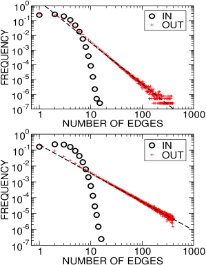
Figure 3: Degree distributions (in logarithmic scale) of two graphs generated with our algorithm. The two panels correspond to graphs having $n=400$, square adjacency matrices and different values of the parameters. Top: $\beta=2.8,\ \alpha=1$. Bottom: $\beta=1.8,\ \alpha=0.2$. To obtain a compact indegree distribution in the case of $\beta\leq 2$ one has to supply smaller values of $\alpha$. The dashed lines are power-laws with exponent $\beta$.

Let us concentrate first on the outdegree. An evaluation of its distribution yields the following asymptotic law for $n\to\infty$ for any $\alpha>0$ and $\beta>1$:

$$P\{S_{n,j}=k\}\sim p_{\alpha,\beta}(k)=\frac{\alpha^{\beta-1}(\beta-1)}{k!}\int_{\alpha}^{+\infty}t^{k-\beta}e^{-t}dt.$$

It is easy to show that $p_{\alpha,\beta}(k)$ has a power-law tail. Indeed, if $k>\beta$, $p_{\alpha,\beta}(k)=\alpha^{\beta-1}(\beta-1)(\frac{\Gamma(k+1-\beta)}{\Gamma(k+1)}-\frac{1}{\Gamma(k+1)}\int_{0}^{\alpha}t^{k-\beta}e^{-t}dt)$ (where $\Gamma$ indicates the gamma function). Thus, since $\frac{\Gamma(k+1-\beta)}{\Gamma(k+1)}\sim\frac{1}{k^{\beta}}$, one concludes that

$$p_{\alpha,\beta}(k)=\frac{1}{k^{\beta}}(\alpha^{\beta-1}(\beta-1)+o(1))\ \ .$$

Fig.3 shows the degree distributions of numerically generated examples for $n=400$. In practice, already at $n\sim 100$ one gets a very marked power-law in the tail of the outdegree distribution. Considering now the indegree, since its behavior is determined by $\mu_{n}$, one has to distinguish among the different possible scalings for this quantity. The simplest case is $\beta>2$, where for $m_{n}=]\delta n[$ ($\delta$ being any constant in $(0,1]$ and $]x[$ being the integer part of $x$) and for $n\to\infty$, using the Poissonian approximation of a binomial distribution, it is immediate to show that $P\{Z_{m_{n},j}=k\}\sim\frac{e^{-\lambda}\lambda^{k}}{k!}$, with $\lambda=\frac{\delta\alpha(\beta-1)}{(\beta-2)}.$ Things are slightly more complicated for $\beta\leq 2$. Here, essentially because of the scaling for $\mu_{n}$ in the limit $n\to\infty$, the indegree distribution diverges if one chooses $m_{n}=]\delta n[$. Thus, to obtain a well-behaved asymptotic distribution, one has to compensate more strongly for the scaling of $\mu_{n}$ with the number of rows of $A$. For $\beta=2$, the necessary choice is $m_{n}=]\delta n/\log n[$ rows, and for $1<\beta<2$ one has to take $m_{n}=]\delta n^{\beta-1}[$ rows. With these prescriptions, the indegree distribution is asymptotically Poisson, and has the form $\frac{e^{-\lambda}\lambda^{k}}{k!}$ with $\lambda=\delta\alpha$, or $\lambda=\delta\alpha^{\beta-1}\frac{\beta-1}{2-\beta}$, for $\beta=2$ and $1<\beta<2$ respectively. In other words, asking for a degree distribution that brings to an outdegree having a power-law tail with divergent mean ($\beta\leq 2$) poses a heavy constraint on the number of regulator nodes (the rows of the matrix). On the other hand, for the purpose of generating square ($n\times n$) matrices at finite $n$ with $\beta\leq 2$ and compact indegree, this issue is not so important. A suitable choice of the parameter $\alpha$ (see Fig. 3) can solve the problem. In what follows we will discuss mainly the case of square matrices.

III.2 Subgraphs.

The simple structure of the random graphs generated by our algorithm makes it possible to compute analytically the mean value of the number of subgraphs of a given shape contained in the graph. Consider a subgraph $H$, with $k$ nodes and $m$ edges, that is, the set of ordered pairs of nodes $H=\{i_{1}\to i_{1,1},\dots,i_{1}\to i_{1,m_{1}},i_{2}\to i_{2,1},\dots,i_{k}\to i_{k,1},\dots,i_{k}\to i_{k,m_{k}}\}$, where $\sum_{i=1}^{k}m_{i}=m$. For example, $i_{1}\to i_{2},i_{2}\to i_{3},i_{3}\to i_{1}$ denotes a “feedback loop” (fbl), or a 3-cycle. Now, if $G_{n}$ is a random graph with $n$ nodes generated by our algorithm, the probability to observe $H$ as a subgraph of $G_{n}$ can be written as

$$P\{H\in G_{n}\}=\int_{[0,1]}\theta_{1}^{m_{1}}\pi(d\theta_{1})\dots\int_{[0,1]}\theta_{k}^{m_{k}}\pi_{n}(d\theta_{k}).$$

To compute the mean of the number $\mathcal{N}_{H}(G_{n})$ of subgraphs isomorphic to $H$ one also has to consider the quantity $N(H)$ of subgraphs isomorphic to $H$ contained in the complete graph with $n$ nodes. The desired average is then $<\mathcal{N}_{H}(G_{n})>=N(H)P\{H\in G_{n}\}$ (where $<..>$ denotes the mean). Things are slightly more complicated for rectangular matrices because in the evaluation of $N(H)$ one needs to take into consideration also the constrains given by the fact that only $m_{n}$ nodes can have out edges.

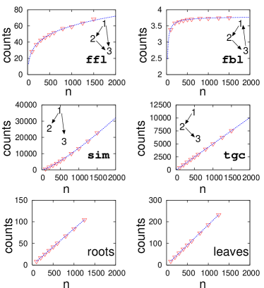
Figure 4: Comparison between analytical (dotted lines) and numerical (triangles) evaluations of the mean number of some observables as a function of system size $n$, for $\beta=2.8,\ \alpha=1$. Numerical averages are evaluated on $10^{5}$ realizations. Top and middle: mean number of three-node subgraphs. Each subgraph is sketched next to its corresponding plot. Top: feedforward and feedback loops (ffl and fbl). Middle: two kinds of open triangles, that can be termed “single input modules” (sim) and “three-gene chains” (tgc). Bottom: roots and leaves.

As an example, we evaluate now, in the case of square matrices, the mean number of feedback loops versus feedforward loops, which play an important role for transcription MA03 . A feedforward loop (ffl) is a triangle with the form $i_{1}\to i_{2}\to i_{3},i_{1}\to i_{3}$. It is found to be a motif in known transcription networks, and identified with the function of persistence filter or amplifier. Conversely, feedback loops (which in principle could form switches and oscillators) are usually not found in transcription networks SMM+02 ; MIK+04 . Following the procedure described above, one gets $<\mathcal{N}_{\mathtt{fbl}}(G_{n})>=2{n\choose 3}\mu_{n}^{3}$ (this holds also for $k$-cycles, with $k$ in place of 3). Once more, this can be evaluated analytically with straightforward calculations. As it depends only on the behavior of $\mu_{n}$, its scaling for large $n$ easily follows. The evaluation of feedforward loops is slightly more complicated. In general

$$<\mathcal{N}_{\mathtt{ffl}}(G_{n})>=6{n\choose 3}\int_{[0,1]}\theta^{2}\pi_{n}(d\theta)\int_{[0,1]}\theta\pi_{n}(d\theta),$$

and hence, under (2),

$$\begin{array}[]{lll}<\mathcal{N}_{\mathtt{ffl}}(G_{n})>&=&6{n\choose 3}\frac{(\beta-1)^{2}}{[(n/\alpha)^{\beta-1}-1]^{2}}\times\\ \\ &&\int_{\alpha/n}^{1}\theta^{2-\beta}d\theta\int_{\alpha/n}^{1}\theta^{1-\beta}d\theta.\end{array}$$

Note that the finite $n$ formulas above can be computed explicitly, and so does their scaling for finite sizes. In appendix A, we spelled out the example of ffls to exemplify this point.

In Fig. 4, we report a comparison of the exact calculation of some triangular subgraphs with results obtained from numerical evaluation. The agreement between the analytical expressions and the numerics is perfect. Having analytically exact expressions for any system size can be an advantage with respect to models where only asymptotically exact expressions are available, especially thinking that many concrete datasets have relatively small sizes. Moreover, it is possible to compute analytically the standard deviation of the number of subgraphs. For example, we considered again the number of feedback loops and feedforward loops. The most interesting fact is that for $\beta>2$, the former are always more widely distributed. A sketch of the calculation and some results are reported in Appendix B.

Finally, one can evaluate the scaling behavior of the ratio of feedback and feedforward loops, which is given below

$$\frac{\langle\mathcal{N}_{\mathtt{ffl}}(G_{n})\rangle}{\langle\mathcal{N}_{\mathtt{fbl}}(G_{n})\rangle}\sim\left\{\begin{array}[]{ll}n^{\beta-1}&\,\,\,\,\mathrm{if}\ \ 1<\beta<2\\ n/(\log n)^{2}&\,\,\,\,\mathrm{if}\ \ \beta=2\\ n^{3-\beta}&\,\,\,\mathrm{if}\ \ 2<\beta<3\\ \log n&\,\,\,\mathrm{if}\ \ \beta=3\\ \lambda&\,\,\,\mathrm{if}\ \ \beta>3\\ \end{array}\right.$$

where $\lambda=3(\beta-2)^{2}(\beta-3)^{-1}(\beta-1)^{-1}>1$. Thus, the ffl always dominate, although there is a wide range of regimes. Note that the dominance of feedforward triangles is even stronger if one considers the rectangular adjacency matrices discussed above. For example, for $1<\beta<2$, and rectangular matrices, we calculate $\frac{\langle\mathcal{N}_{\mathtt{ffl}}(G_{n})\rangle}{\langle\mathcal{N}_{\mathtt{fbl}}(G_{n})\rangle}\sim n$.

III.3 Roots and Leaves.

As a second example, we report the calculation of the mean number of roots (nodes with only outgoing links) versus leaves (nodes with only incoming links). More specifically, we say that $i$ is a root if there is no edge of the kind $j\to i$, but there is at least one edge of the kind $i\to j$, with $j\not=i$. Loops do not count. Conversely, we say that $i$ is a leaf if there is no edge of the kind $i\to j$, but there is at least one edge of the kind $j\to i$, with $j\not=i$. Again we exclude loops and isolated points. We find the following scaling for the numbers of roots $\mathfrak{R}$, and of leaves $\mathfrak{L}$:

$$<\mathfrak{L}(G_{n})>\sim n$$

while

$$<\mathfrak{R}(G_{n})>\sim\left\{\begin{array}[]{ll}n&\,\,\mathrm{if}\ \ \beta>2\\ n^{1-\alpha}&\,\,\mathrm{if}\ \ \beta=2\\ e^{-\tau^{2}n^{2-\beta}}&\,\,\mathrm{if}\ \ 1<\beta<2\\ \end{array}\right.$$

where $\tau^{2}=\frac{\beta-1}{2-\beta}\alpha^{\beta-1}$. Once again, we stress that these quantities are accessible analytically, and there is perfect agreement between the data generated by the algorithm and the calculations.

III.4 Hub.

As a last example of important observable in our graph ensemble, we discuss the distribution and mean number of hubs. The so–called hub is the node having maximal outdegree among the nodes, that is, $H_{n}:=\max_{i=1,\dots,m_{n}}(S_{n,i})$. Once again, it is possible to give an analytical expression of the limit law of the hub under a suitable rescaling. Indeed, by stochastic independence, it is clear that $P\{H_{n}\leq xb_{n}\}=(1-P\{S_{n,i}>xb_{n}\})^{m_{n}}$, where $x>0$ is any positive number. Moreover, it is not too hard to prove that, for suitable choices of $b_{n}$ and $m_{n}$, $P\{S_{n,i}>xb_{n}\}=1/m_{n}[(\alpha/x)^{\beta-1}+o(1)]$. More precisely, for $\beta\geq 2$ and for every positive number $x$

$$P\{H_{n}/b_{n}\leq x\}\sim e^{-(\alpha/x)^{\beta-1}}.$$

The above expression gives the effective probability distribution that one can use for the hub outdegree in the asymptotic limit. In particular, for $\beta>2$, $m_{n}=n$ and $b_{n}=n^{1/(\beta-1)}$, and, with some work, we prove that $<H_{n}>\sim n^{1/(\beta-1)}$, as found in IMK+03 . For $\beta=2$, one has to take $m_{n}=b_{n}=n/\log n$, which lead to analogous scaling results. Finally, for $1<\beta<2$ and $m_{n}=n^{\beta-1}$, one gets the expression

$$P\{H_{n}/n\leq x\}\sim e^{-(\alpha/x)^{\beta-1}}\chi_{(0,1)}(x)+\chi_{[1,\infty)}(x)$$

for every positive $x$. Note that in this last case the probability of finding a hub of size $n$ is asymptotically finite, and equal to $1-e^{-(\alpha)^{\beta-1}}$. This concentration effect was already noted in IMK+03 using a different random graph model, without computing explicitly the asymptotic probability distribution. It is worth recalling that $e^{-(\alpha/x)^{\beta-1}}\mathbb{I}_{[0,+\infty)}(x)$ is the Frechet type II extreme value distribution, i.e. one of the three kinds of extreme value distributions that can arise from limit law of maximum of independent and identically distributed random variables (see for instance galambos ). For extreme values distributions in scale-free network models see, e.g., moreira .

IV Other Applications.

While here we restricted our attention to the case of directed graphs with compact indegree and power-law outdegree, our coin-toss method of generating exchangeable graphs is more general and has a wider range of application. For example, one can consider the following algorithm: (i) throw a bias $\theta$ from a prescribed probability distribution $\pi_{n}$ (ii) set all the elements of $A$ to be $0$ or $1$ according to the toss of a coin with bias $\theta$. The resulting probability law, for square matrices, is

$$\begin{split}Q\{x_{i,j}=e_{i,j};&\,i,j=1,\dots,n\}=\\ &\int_{[0,1]}\theta^{\sum_{i,j}e_{i,j}}(1-\theta)^{n^{2}-\sum_{i,j}e_{i,j}}\pi_{n}(d\theta)\\ \end{split}$$

$e_{i,j}$ being any element in $\{0,1\}$ $i,j=1,\dots n$. Again set $\mu_{n}:=Q\{x_{i,j}^{(n)}=1\}=\int_{[0,1]}\theta\pi_{n}(d\theta)$. The resulting ensemble of random graph has a large variability in the number of links. In the $n\times n$ case, the degree distributions are given by $Q\{S_{n,i}=k\}=Q\{Z_{n,j}=k\}={{n}\choose{k}}\int_{[0,1]}\theta^{k}(1-\theta)^{n-k}\pi_{n}(d\theta).$ Assuming (2) one gets

$$Q\{S_{n,j}=k\}\sim Q\{Z_{n,i}=k\}\sim p_{\alpha,\beta}(k),$$

which has, again, a power-law tail. For this model, quantities like the mean number of subgraphs, roots, leaves and hubs, are again easily computed analytically, in the same way we described above. Furthermore, throwing a triangular matrix with the same algorithm, one can easily generate a power-law model for undirected graphs. Finally, variants of the model can be generated by changing the probability distribution $\pi_{n}$ for the biases. Overall, all these possibilities remain open to explore and could be useful to generate both analytically solvable random graph models and quicker algorithms in many applications.

V Example of Comparison with Empirical Data.

A detailed comparison between known real transcriptional networks and the null models obtained with our coin-toss algorithm is beyond our aims here. Nevertheless, to show that our model can be used for direct statistical comparisons, as an alternative to the more stringent constraint of preserved degree sequences, we present here a brief application to the Shen-Orr SMM+02 dataset for the E. coli Transcription Network. Motifs discovery, for example, entails comparing the occurrence of subgraphs in a real network with a null ensemble. This null ensemble can be obtained from our coin-toss model, with some prescribed parameter set. The parameters can be chosen by performing a fit of the model graphs with some observed features of the data, such as, for example, decay of the degree distributions and number of regulatory elements (additional parameters can also be introduced if needed). The chosen “invariants” can be motivated biologically.

We generated our random ensemble with distribution $\pi_{n}$ given by (3) as follows. First, from a frequentistic estimate of $\pi_{n}$ we determined the probable value of $\beta$ and of the cutoff on the maximum, i.e. $\gamma$. This last quantity has to be regarded as a biological constraint, and is necessary to obtain an ensemble having on average the same number of links as the empirical one; we measure the upper cutoff $1-\gamma/n$ to be about $18\%$. The estimated value for $\beta$ ranges from 1.6 to 2.1, depending on the binning of the histogram of $\pi_{n}(\theta)$. We note that these values are larger than those that obtained from fitting direcly on the outdegree sequence. As a second step, we fixed the rectangularity of the matrix with the ratio of transcription factors to total number of nodes, choosing $\delta$ such that $m_{n}/n\simeq 0.2766$. Finally, we fitted $\alpha$ to reproduce on average the observed number of links and nodes. In practice, since the model nturally produces a certain number of isolated nodes, one has to generate slightly larger matrices and compare the submatrix made of non-isolated nodes.

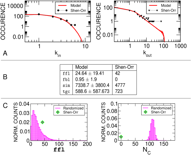
Figure 5: Application of the model to the Shen-Orr dataset. Example of fit and observed features. The plots refer to the parameter set $\beta=1.83,\alpha=0.5,m_{n}/n=0.2766$, with a cutoff on the maximum outdegree at $18\%$ of the nodes as described in the text. (A) in- and out-degree histograms of the empirical graph, compared to the random ensemble. While the tail of the outdegree may not seem a good fit, we note that the integral of the $>13$ tail, or the estimated number of “global regulators”, of the two laws are remarkably similar (8 in the empirical graph vs 9.7 in the randomized network) so that this has to be regarded as a good agreement. (B) Table comparing the subgraph content (for the three-node subgraphs analyzed here) of the model graphs with the empirical one. The two quantities are in general very similar, with the exception of the ffl, which deviates from average, but only slightly. (C) The feedback in the graph deviates from average more than the triangular subgraphs. Left panel: the distribution of ffls compared with the empirical value. Right panel: the feedback of the random and empirical graphs differ. $N_{C}$ Measures the number of nodes left in a graph after pruning the input and output trees, as described in gammachi .

The ensemble obtained with this procedure fits quite well the empirical in- and out-degree sequences (Fig. 5A), Also, the model reproduces the empirical number of transcription factors, roots and leaves as average values. As a remark, we note that, unless new prescriptions for the generation of the graphs, and thus new parameters, are introduced, roots, leaves and transcripiton factors cannot be reproduced well with smaller values of $\beta$ than the ones we used. One can take this as a confirmation that the range of values for the exponent obtained with our fitting procedure are reasonable.

We also measured the three-node subgraph content of the null model and compared it with the empirical data and the model ensemble are very close (Fig. 5B). The only exception is the ffl, with a slight deviation, that, however, is much less significant than with the degree-conserving ensemble. Thus, in term of these observables, one obtains similar graphs as the empirical one. This means that in the resulting ensemble the average motif content can be regarded as an invariant, rather than as an observable. Finally, we quantified the feedback properties (Fig. 5C). In order to do this, we measured the number $N_{C}$ of nodes left in the graph after pruning its input and output tree-like components with an iterative decimation algorithm gammachi ; pnas . In particular, none of the graphs we generated was treelike and feedforward as the empirical one. One may then speculate that the motif content and the hierarchical properties, two important properties are somehow related.

VI Conclusions.

We presented an algorithmic way to generate directed graphs with, asymptotically, power-law outdegree and compact indegree, easily generalizable to different kinds of graphs. The discussion was carried out having in mind an application in the realm of transcription networks, although there are many possible connections with other experimentally accessible complex networks, including biological ones. Compared to other techniques, our model has the advantage to be quick in generating large graphs, as it is not designed to preserve a prescribed degree sequence, but rather to generate an ensemble with given degree distributions. As such, it is an interesting tool to characterize topological observables in large graphs. Most importantly, many of the relevant observables are accessible analytically, for any value of $n$. We supplied here as an example the evaluation of the mean number of subgraphs, roots and leaves and hub.

We should add here a comment regarding the is not evident that the proposed approach is more efficient that the Molloy-Reed algorithm MR95 , which generates “stubs” with desired in- and outdegree sequences, and matches the stubs to generate the graphs. This model could be re-cast to be similar in spirit, in the sense that one could fix the relevant distributions depending on parameters, ad throw the degree sequences from the distributions. Once the number of connections for each node has been drawn from the expected degree distribution and without avoiding multiple connections, the computational cost of pairing the stubs is order E (number of edges), so in sparse networks this could be less than order $n^{2}$, and in non-sparse networks it could be $n^{2}$. Despite the algorithm suffers from the undesired production of multiple edges, due to the computational complexity of pairing hubs, for a compact indegree distribution, this computational cost can be small CFS05 , allowing a practical applicability in some regimes. On the other hand, we think that our approach remains competitive, as its computational cost is not affected by the complexity of the graph ensemble, and, as we have shown, is very versatile for analytical calculations.

Regarding the subgraph structure, we note that while ffls always dominate on fbls, there are qualitatively different behaviors depending on the exponent $\beta$. The most marked dominance is found for smaller values of $\beta$, and is further increased by considering rectangular matrices (i.e. asymptotically compact indegree). Thus, the degree distribution poses some important constraints on the dominant subgraphs in our null model. We would like to spend a few more words on these scaling laws with system size $n$. In our model the scaling of $\mu_{n}$ with the decay exponent $\beta$ pilots the transitions of all the observables. In particular, it renders necessary to consider rectangular matrices to obtain an asymptotically compact indegree if $\beta\leq 2$.

This behavior is interesting on theoretical grounds, and shows how much the distributions for the in- and outdegree in transcription networks are strongly unbalanced. For example, in the model described in section IV, where the indegree is allowed to have a power-law tail, the situation is rather different. In the case of transcription networks, there is an observed scaling law of the fraction of transcription factors (nodes that have at least one outgoing link). This is a power-law $n^{\zeta}$ vN03 with positive exponent $1<\zeta<2$. Looking at the distribution of roots, one easily realizes that this behavior forbids any asymptotic limit assuming the graph structure of our model, and is thus incompatible with it. At the light of our calculations, we can observe that it is likely that for larger values of $n$ the outdegree ceases to follow a power-law, and/or the average indegree ceases to be finite, the opposite trend to that observed in small networks. Experimental observations of larger transcription networks will elucidate this question.

We should stress here that the above considerations apply mainly to the model. Nevertheless, we showed that in principle our model can be used for direct statistical comparisons, as an alternative to the more stringent constraint of preserved degree sequences. An example of such a fitting procedure, produced an ensemble of networks that resemble the empirical one of E. coli in terms of degree distribution, number of links, roots, leaves and transcrption factors. Interestingly, the null ensemble produced this way also has a very similar three-node subgraph content as the empirical graph. On the other hand, the feedback properties are very different. The outcome of such a comparison might depend on the invariance criteria used for the fitting. This is an interesting feature that can be used to produce flexible null models, depending on the quantities of interest. On the other hand, this feature makes the handling of the model more delicate than the standard degree-conserving randomizations. In particular, a more exhaustive analysis than that presented here is needed to draw clearcut conclusions on experimental graphs in_prep . Clearly, the degree sequences of, for example, the E. coli network, are not stringently fixed by any physical of biological constraint. Rather, the network, during evolution (and within a population), moves in a larger “space of possible interactions”, determined by selective pressure and other biological constraints, which has not been strictly identified yet. Generalizations of our null model might help exploring this evolutionary problem.

Finally, we showed how the coin-toss algorithm, or exchangeable graph model, has a wider range of application than the main example examined here. To illustrate this, we explained how, with the same technique, one can obtain directed and undirected power-law random graphs. Obviously, the range of possibilities is even larger if one starts to play with the probability distribution for the biases $\pi_{n}(d\theta)$. For this reason, on more abstract grounds, the model can be useful in the context of the theory of correlated random networks MS05 ; BL02 . It is a quick algorithm easy to implement and to analyze theoretically. Indeed, because of its simple formulation, the potential for further analytical calculations is large. For example, one can evaluate the kernel of $A$, which is useful in connection with problems of the Satisfiability class, which have seldom been analyzed on non-Poisson random graphs Kol98 ; Lev05 ; MPZ02 ; LJB05 .

Appendix A Average of ffl

This appendix reports in more detail the calculation of the mean number of ffls for $1<\beta<2$. Starting from the definition, we obtain with straightforward calculations

$$\begin{split}&<\mathcal{N}_{\mathtt{ffl}}(G_{n})>\\ &=6{n\choose 3}\frac{(\beta-1)^{2}}{[(n/\alpha)^{\beta-1}-1]^{2}}\int_{\alpha/n}^{1}\theta^{2-\beta}d\theta\int_{\alpha/n}^{1}\theta^{1-\beta}d\theta\\ &=\frac{\alpha^{2\beta-2}(\beta-1)}{(3-\beta)(2-\beta)}n^{5-2\beta}\left[1-\frac{3}{n}+\frac{2}{n^{2}}\right]\\ &\times\left[1-\left(\frac{\alpha}{n}\right)^{3-\beta}-\left(\frac{\alpha}{n}\right)^{2-\beta}+\left(\frac{\alpha}{n}\right)^{5-2\beta}\right]\\ \end{split}$$

Note that, since the finite $n$ formula for the mean is known exactly, the finite size scaling can be computed analytically, simply by isolating the leading terms in the approach to the asymptotic limit. For example, in the case of the ffl average computed above, one has

$$\begin{split}<\mathcal{N}_{\mathtt{ffl}}(G_{n})>&=\frac{\alpha^{2\beta-2}(\beta-1)}{(3-\beta)(2-\beta)}n^{5-2\beta}\\ \times&\left[1-\left(\frac{\alpha}{n}\right)^{2-\beta}+o\left(\frac{1}{n^{2-\beta}}\right)\right].\\ \end{split}$$

Appendix B Variance of fbl vs ffl.

We report here the calculation of the standard deviation of feedforward and feedback loops, in the case of square matrices. The key point is to evaluate $\langle\mathcal{N}_{\mathtt{ffl}}(G_{n})^{2}\rangle$ and $\langle\mathcal{N}_{\mathtt{fbl}}(G_{n})^{2}\rangle$. Again, for the sake of simplicity, we will deal only with square matrices. It is clear that $\langle\mathcal{N}_{\mathtt{fbl}}(G_{n})^{2}\rangle=\sum_{t\in\tau}\sum_{s\in\tau}P\{s,t\in G_{n}\}$, $\tau$ being the set of all feedback loops contained in the complete $n$ graph. Analogously one obtains $\langle\mathcal{N}_{\mathtt{fll}}(G_{n})^{2}\rangle$ taking as $\tau$ the set of all feedforward loops. Simple calculations give

$$\begin{split}\langle\mathcal{N}_{\mathtt{fbl}}(G_{n})^{2}\rangle&=4{n\choose 3}{n-3\choose 3}\mu_{n}^{6}+12{n\choose 3}{n-3\choose 2}\mu_{n}^{2}\delta_{2,n}\\ &+6(n-3){n\choose 3}(\mu_{n}^{3}+\mu_{n}^{2}\delta_{2,n}^{2})+2{n\choose 3}\mu_{n}3\\ \end{split}$$

where $\delta_{i,n}:=\int_{0}^{1}\theta^{i}\pi_{n}(d\theta)$. Hence, one obtains

$$Var(\mathcal{N}_{\mathtt{fbl}}(G_{n}))\sim\left\{\begin{array}[]{ll}n^{5(2-\beta)}&\,\,\,\,\mathrm{if}\ \ 1<\beta<2\\ (\log n)^{4}&\,\,\,\,\mathrm{if}\ \ \beta=2\\ \frac{1}{3}(\alpha\frac{\beta-1}{\beta-2})^{3}&\,\,\,\mathrm{if}\ \ \beta\geq 2\\ \end{array}\right.$$

As for $\mathcal{N}_{\mathtt{ffl}}$, the computations are longer, but essentially the same. The problem is that $P\{s,t\in G_{n}\}$ can take many different expression depending on $s$ and $t$. With some simple but tedious calculations one gets

$$\begin{split}<\mathcal{N}_{\mathtt{ffl}}(G_{n})^{2}>&=6{n\choose 3}A_{n}+6(n-3){n\choose 3}B_{n}\\ &+12{n\choose 3}{n-3\choose 2}C_{n}+36{n\choose 3}{n-3\choose 3}D_{n}\\ \end{split}$$

with $A_{n}=\delta_{1,n}\delta_{2,n}+\delta_{2,n}^{2}+\delta_{1,n}^{2}\delta_{2,n}$, $B_{n}=\delta_{2,n}\delta_{3,n}+5\delta_{1,n}\delta_{2,n}^{2}+3\delta_{1,n}^{2}\delta_{3,n}+\delta_{3,n}^{2}+2\delta_{1,n}\delta_{2,n}\delta_{3,n}+2\delta_{2,n}^{3}+4\delta_{1,n}^{2}\delta_{2,n}^{2}$, $C_{n}=2\delta_{1,n}\delta_{2,n}\delta_{3,n}++\delta_{1,n}^{2}\delta_{4,n}+5\delta_{1,n}^{2}\delta_{2,n}+\delta_{2,n}^{3}$ and $D_{n}=\delta_{1,n}^{2}\delta_{2,n}^{2}$. Hence,

$$\begin{split}Var(\mathcal{N}_{\mathtt{ffl}}(G_{n}))&=6{n\choose 3}A_{n}+6(n-3){n\choose 3}B_{n}\\ &+12{n\choose 3}{n-3\choose 2}C_{n}-36R_{n}D_{n}\\ \end{split}$$

with $R_{n}=[{n\choose 3}-{n-3\choose 3}]$. For example, if $2<\beta<3$, the last expression gives

$$Var(\mathcal{N}_{\mathtt{fll}}(G_{n}))\sim n^{2(\beta+1)}.$$

References

- (1) M. Babu, N. Luscombe, L. Aravind, M. Gerstein, S. Teichmann, Curr Opin Struct Biol 14, 283 (2004).
- (2) T. Lee, et al., Science 298, 799 (2002).
- (3) N. Guelzim, S. Bottani, P. Bourgine, F. Kepes, Nat Genet 31, 60 (2002).
- (4) H. Salgado, et al., Nucleic Acids Res 29, 72 (2001).
- (5) C. Harbison, et al., Nature 431, 99 (2004).
- (6) R. Milo, et al., Science 298, 824 (2002).
- (7) R. Milo, et al., Science 303, 1538 (2004).
- (8) A. Mazurie, S. Bottani, M. Vergassola, Genome Biol 6, R35 (2005).
- (9) D. Wolf, A. Arkin, Curr Opin Microbiol 6, 125 (2003).
- (10) E. Yeger-Lotem, et al., Proc Natl Acad Sci U S A 101, 5934 (2004).
- (11) S. Itzkovitz, R. Milo, N. Kashtan, G. Ziv, U. Alon, Phys Rev E 68, 026127 (2003).
- (12) J.Galambos, The asymptotic theory of extreme order statistics. R.E. Krieger Publishing Co., Inc., Melbourne, FL, (1987).
- (13) A.A. Moreira, J.S. Andrade, and N.A. Nunes Amaral, Phys Rev Lett. 89, 268703 (2002).
- (14) M. Cosentino Lagomarsino, B. Bassetti, P. Jona, Soft Condensed Matter: New Research (Nova Science Publishers, 2005). (q-bio.MN/0502017).
- (15) S. Mangan, U. Alon, Proc Natl Acad Sci U S A 100, 11980 (2003).
- (16) D. Braha, Y. Bar-Yam Phys Rev E 69, 016113 (2004).
- (17) A. Rao, R. Jana, S. Bandyopadhyay, Indian J. Stat. 58(A), 225 (1996).
- (18) Y. Chen, P. Diaconis, S. Holmes, J. Liu, J. Amer. Statistical Assoc. 100, 109 (2005).
- (19) R. Milo, N. Kashtan, S. Itzkovitz, M. E. J. Newman, U. Alon, cond-mat/0312028 (2003).
- (20) M. Molloy and B. Reed, Random Structures and Algorithms 6, 161-179 (1995).
- (21) In mathematical terms, one says that each row is exchangeable with de Finetti measure .
- (22) S. Maslov, K. Sneppen Phys Biol 2 (4), S94 (2005).
- (23) M. Newman, Phys Rev Lett 89, 208701 (2002).
- (24) G. Caldarelli, A. Capocci, P. De Los rios, M.A. Munoz, Phys Rev Lett 89, 258702 (2002).
- (25) B.Söderberg, Phys Rev E 66, 066121 (2002).
- (26) M. Boguña, R. Pastor-Satorras, Phys Rev E 68, 036112 (2003).
- (27) S. Shen-Orr, R. Milo, S. Mangan, U. Alon, Nat Genet 31, 64 (2002).
- (28) M. Boguña, R. Pastor-Satorras and A. Vespignani. Eur. Phys. J. B 38 (2004) p. 205.
- (29) E. van Nimwegen, Trends Genet 19, 479 (2003).
- (30) J. Berg and M. Lässig, Phys. Rev. Lett. 89(22), 228701 (2002)
- (31) V. F. Kolchin, Random Graphs (Cambridge University Press, New York, 1998).
- (32) A. A. Levitskaya, Cybernetics and System Analysis 41, 67 (2005).
- (33) M. Mezard, G. Parisi, R. Zecchina, Science 297, 812 (2002).
- (34) M. C. Lagomarsino, P. Jona, B. Bassetti, Phys Rev Lett 95, 158701 (2005).
- (35) Cosentino Lagomarsino, M., Bassetti B., Jona P., Lecture Notes in Bioinformatics, Proceedings of the CMSB conference 2006. Springer-Verlag, 2006 (q-bio.MN/0606039).
- (36) Cosentino Lagomarsino M., Jona. P. Bassetti, B., and Isambert, H., Proc Natl Acad Sci U S A, 104 13, 5517, 2007 (q-bio.MN/0701035).
- (37) Cosentino Lagomarsino, M., Bassetti F. In preparation (2007).