Dynamics of a quantum phase transition in the random Ising model

Abstract

A quantum phase transition from paramagnetic to ferromagnetic phase is driven by a time-dependent external magnetic field. For any rate of the transition the evolution is non-adiabatic and finite density of defects is excited in the ferromagnetic state. The density of excitations has only logarithmic dependence on the transition rate. This is much weaker than any usual power law scaling predicted for pure systems by the Kibble-Zurek mechanism.

PACS numbers: 03.65.-w, 73.43.Nq, 03.75.Lm, 32.80.Bx, 05.70.Fh

According to the book [1] our understanding of quantum phase transitions is based on two prototypical models: the quantum Ising chain and the Bose-Hubbard model. It is well established in the exactly solvable Ising model [5, 6, 7] and there are indications in the Bose-Hubbard model [8] that essential properties of a dynamical quantum phase transition are captured by the Kibble-Zurek (KZ) mechanism of defect formation [2]. This theory was originally developed for thermodynamic transitions and tested both by numerical simulations [3] and by experiments in finite-temperature condensed matter systems [4]. It is based on the observation that, because of the critical slowing down, a system driven across its critical point must go out of thermal equilibrium no matter how slow is the transition rate. Using only combination of general casuality and universality arguments it shows that in a transition from a disordered to ordered phase the system ends in a non-equilibrium state with finite ordered domains of average size

$$\hat{\xi}~{}\simeq~{}\tau_{Q}^{\frac{\nu}{z\nu+1}}~{}.$$ (1)

Here $z$ and $\nu$ are critical exponents and $\tau_{Q}$ is time of the transition (or quench). No matter how slow is the transition the system does not have enough time to order throughout its whole volume and average size of ordered domains is limited to a finite $\hat{\xi}$ which is a power of the transition time $\tau_{Q}$.

The short list of the two prototypical models must be supplemented by a prototypical disordered system i.e. the random Ising chain defined by the Hamiltonian [10, 11]

$$H~{}=~{}-\sum_{n=1}^{N}\left(h~{}\sigma^{x}_{n}+J_{n}~{}\sigma^{z}_{n}\sigma^{z}_{n+1}\right)~{}.$$ (2)

with periodic boundary conditions

$$\vec{\sigma}_{N+1}~{}=~{}\vec{\sigma}_{1}~{}.$$ (3)

Here $J_{n}$’s are random ferromagnetic couplings, $J_{n}>0$, and $h$ is external magnetic field. This model has a quantum critical point at $h_{c}=\exp\left(\overline{\ln J_{n}}\right)$ separating ferromagnetic ($h<h_{c}$) from paramagnetic ($h>h_{c}$) phase. When $h\to\infty$ the ground state becomes fully polarized along the $x$-axis,

$$\left|\rightarrow\rightarrow\rightarrow\rightarrow\rightarrow\rightarrow\dots\right\rangle~{},$$ (4)

but when $h=0$ there are two degenerate ferromagnetic ground states

$$\left|\uparrow\uparrow\uparrow\uparrow\uparrow\uparrow\dots\right\rangle~{},~{}~{}~{}~{}~{}\left|\downarrow\downarrow\downarrow\downarrow\downarrow\downarrow\dots\right\rangle~{}.~{}$$ (5)

The critical point at $h_{c}$ is surrounded by the Griffith regime (or phase) of infinite linear susceptibility.

The random Ising model is important because real condensed matter spin systems are random. Their randomness is not a mere small perturbation on top of pure models because the disorder is changing their universality class. For example, the randomness of $J_{n}$ in the model (2) is changing its universality class with respect to the pure Ising chain with a constant $J_{n}=J$. No matter how weak is the randomness of $J_{n}$ renormalization group transformations drive the model towards an infinite disorder fixed point [11]. As a result, the random Ising chain has $\nu=2$ instead of $\nu=1$ and, more importantly, $z\to\infty$ instead of $z=1$. The diverging dynamical exponent marks a qualitative difference between the pure and the disordered model. As the dynamical exponent is relevant to dynamical phase transitions, its singularity is suggesting that an outcome of the transition in a disordered system can be qualitatively different from that in its pure counterpart. This expectation has never been tested in the theory of dynamical phase transitions.

In the model (2) a dynamical paramagnet-ferromagnet transition is not adiabatic and, as a result, the state after transition is a superposition over excited states like

$$\left|\uparrow\uparrow\uparrow\uparrow\uparrow\uparrow\downarrow\downarrow\downarrow\downarrow\downarrow\downarrow\downarrow\uparrow\uparrow\uparrow\uparrow\uparrow\downarrow\downarrow\downarrow\downarrow\downarrow\dots\right\rangle$$ (6)

with finite ferromagnetic domains separated by domain walls or kinks. The diverging dynamical exponent $z$ implies that, in first approximation, the size of the ordered domains $\hat{\xi}$ in Eq.(1) does not depend on the quench time. No matter how slow is the transition the average density of kinks $d\sim\hat{\xi}^{-1}$ remains the same.

In second approximation we can follow general principles of the KZ mechanism [2] to derive $\hat{\xi}$ when $z\to\infty$. These ideas were originally proposed for classical transitions [2], but they were generalized recently to quantum phase transitions [8, 9, 5, 6]. The basic idea is that when a system is driven through a quantum phase transition, then the evolution of its state is adiabatic when the system is away from the critical point, but it must be non-adiabatic in a neighborhood of the critical point where the gap $\Delta$ between the ground state and the first excited state tends to zero. It is convenient to measure the distance from the critical point by a dimensionless parameter $\epsilon~{}=~{}\frac{h_{c}-h}{h_{c}}.$ The evolution is non-adiabatic between $-\hat{\epsilon}$ and $+\hat{\epsilon}$, where $\pm\hat{\epsilon}$ are the two points when transition rate equals the gap $\Delta$. On one hand, assuming that $\epsilon(t)$ can be linearized near $\epsilon=0$,

$$\epsilon(t)~{}\simeq~{}\frac{t}{\tau_{Q}}~{},$$ (7)

we can estimate the rate as $\left|\frac{\dot{\epsilon}}{\epsilon}\right|\approx\frac{1}{\tau_{Q}|\epsilon|}$. On the other hand, we know that for $|\epsilon|\to 0$ the gap behaves like

$$\Delta~{}\simeq~{}|\epsilon|^{z\nu}~{}\simeq~{}|\epsilon|^{1/|\epsilon|}~{},$$ (8)

see Ref.[11]. The rate and the gap equal at $\hat{\epsilon}$ when

$$\frac{\alpha}{\tau_{Q}\hat{\epsilon}}~{}=~{}\hat{\epsilon}^{1/\hat{\epsilon}}~{}.$$ (9)

Here $\alpha={\cal O}(1)$ is a single fitting parameter. Quick analysis of this equation shows that $\hat{\epsilon}\to 0$ when $\tau_{Q}\to\infty$: for very slow transitions the evolution is non-adiabatic only in a very close neighborhood of the critical point, where we can use Eq.(8) self-consistently.

In the adiabatic-impulse approximation the state of the system follows its instantaneous ground state before $-\hat{\epsilon}$, then its evolution becomes impulse between $-\hat{\epsilon}$ and $+\hat{\epsilon}~{}$ when the state does not change because reaction of the system is too slow as compared to the transition rate, and finally the evolution becomes adiabatic again after $+\hat{\epsilon}$. Accuracy of the adiabatic-impulse approximation was tested in the quantum context in Refs.[7, 9]. The state of the system at $-\hat{\epsilon}$ is the ground state with a finite correlation length

$$\hat{\xi}~{}=~{}\frac{1}{\hat{\epsilon}^{\nu}}~{}.$$ (10)

This state does not change until $+\hat{\epsilon}$ when the evolution becomes adiabatic again. In this way the correlation length $\hat{\xi}$ becomes imprinted on the state of the system after the transition. This length becomes the average size of ordered domains in the final ferromagnetic state (6). For example, in the random Ising model ($\nu=2$) approximate solution of Eq.(9) in the limit of $\tau_{Q}\to\infty$ together with Eq.(10) gives

$$\hat{\xi}~{}\sim~{}\ln^{2}\tau_{Q}~{}$$ (11)

when $\ln\tau_{Q}\gg 1$. Again, as in our first approximation, the dependence on $\tau_{Q}$ is very weak as compared to any power law scaling.

As mentioned before, validity of Eq.(8) is limited only to close vicinity of the critical point. Further away from this point we can expect spectral properties of the model to be more like in the pure Ising model. This must be true at least for weak disorder, when the random $J_{n}$’s have a narrow distribution around a finite $J$. As a result, for moderately slow transitions, when $\hat{\epsilon}$ is large enough, we can expect

$$\hat{\xi}~{}\sim~{}\tau_{Q}^{1/2}~{},$$ (12)

like in the pure Ising model with $\nu=z=1$ [5, 6], see Eq.(1).

Before proceeding with numerical simulations of a dynamical transition we need better understanding of spectral properties of the random Ising chain. To this end I assume for convenience that $N$ is even and make the Jordan-Wigner transformation,

$$\sigma^{x}_{n}~{}=~{}1-2c^{\dagger}_{n}c_{n}~{},$$ (13)

$$\sigma^{z}_{n}~{}=~{}-\left(c_{n}+c_{n}^{\dagger}\right)\prod_{m<n}(1-2c^{\dagger}_{m}c_{m})~{},$$ (14)

introducing fermionic operators $c_{n}$, which satisfy anticommutation relations $\left\{c_{m},c_{n}^{\dagger}\right\}=\delta_{mn}$ and $\left\{c_{m},c_{n}\right\}=\left\{c_{m}^{\dagger},c_{n}^{\dagger}\right\}=0$. The Hamiltonian (2) becomes

$$H~{}=~{}P^{+}~{}H^{+}~{}P^{+}~{}+~{}P^{-}~{}H^{-}~{}P^{-}~{},$$ (15)

where

$$P^{\pm}=\frac{1}{2}\left[1\pm\prod_{n=1}^{N}\sigma^{x}_{n}\right]=\frac{1}{2}\left[1~{}\pm~{}\prod_{n=1}^{N}\left(1-2c_{n}^{\dagger}c_{n}\right)\right]$$ (16)

are projectors on subspaces with even ($+$) and odd ($-$) numbers of $c$-quasiparticles and

$$H^{\pm} = \sum_{n=1}^{N}\left(hc_{n}^{\dagger}c_{n}-J_{n}c_{n}^{\dagger}c_{n+1}-J_{n}c_{n+1}c_{n}-\frac{h}{2}\right)~{}+$$ (18)

$$~{}{\rm h.c.}~{}$$

are corresponding reduced Hamiltonians. The $c_{n}$’s in $H^{-}$ satisfy periodic boundary conditions $c_{N+1}=c_{1}$, but the $c_{n}$’s in $H^{+}$ must obey $c_{N+1}=-c_{1}$, what I call “antiperiodic” boundary conditions.

The parity of the number of $c$-quasiparticles is a good quantum number and the ground state has even parity for any value of $h$. Assuming that the quench begins in the ground state we can confine to the subspace of even parity. In this subspace the quadratic $H^{+}$ is diagonalized by a Bogoliubov transformation

$$c_{n}~{}=~{}\sum_{m=1}^{N}\left(u_{nm}\gamma_{m}+v^{*}_{nm}\gamma_{m}^{\dagger}\right)$$ (19)

The index $m$ numbers Bogoliubov modes which are eigenmodes with positive $\omega$ of the stationary Bogoliubov-de Gennes equations

$$\omega u_{n}=$$ (20)

$$2hu_{n}-j_{n}\left(u_{n+1}+v_{n+1}\right)+j_{n-1}\left(v_{n-1}-u_{n-1}\right)~{},$$ (21)

$$\omega v_{n}=$$ (22)

$$-2hu_{n}+j_{n}\left(v_{n+1}+u_{n+1}\right)+j_{n-1}\left(v_{n-1}-u_{n-1}\right)~{}.$$ (23)

Here I suppressed the mode number $m$ and defined $j_{n}=J_{n}$ for $n<N$ and $j_{N}=-J_{N}$ to take into account the antiperiodic boundary conditions. The eigenstates $(u_{nm},v_{nm})$ with positive energy $\omega_{m}>0$, normalized so that $\sum_{n}\left(|u_{nm}|^{2}+|v_{nm}|^{2}\right)=1$, define quasiparticle operators $\gamma_{m}=u_{nm}^{*}c_{n}+v_{nm}c_{n}^{\dagger}$. Each positive energy eigenstate has a partner $(u^{-}_{nm},v^{-}_{nm})=(v_{nm},u_{nm})$ with negative energy $-\omega_{m}$ which defines a quasiparticle operator $\gamma_{m}^{-}=(u^{-}_{nm})^{*}c_{n}+v^{-}_{nm}c_{n}^{\dagger}=\gamma_{m}^{\dagger}$. After the transformation (19) the Hamiltonian $H^{+}=\frac{1}{2}\sum_{m=1}^{N}\epsilon_{m}\left(\gamma_{m}^{\dagger}\gamma_{m}-\gamma_{m}^{-\dagger}\gamma_{m}^{-}\right)$ equivalent to

$$H^{+}=\sum_{m=1}^{N}\epsilon_{m}~{}\left(\gamma_{m}^{\dagger}\gamma_{m}-\frac{1}{2}\right)~{}$$ (24)

which is a simple-looking sum of quasiparticles. However, thanks to the projection $P^{+}~{}H^{+}~{}P^{+}$ in Eq.(15) only states with even numbers of quasiparticles belong to the spectrum of $H$.

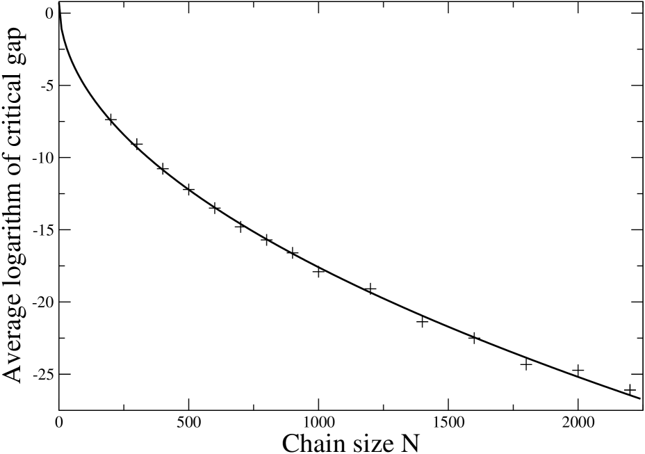
FIG. 1.: Average logarithm of the critical gap $\overline{\ln\Delta_{c}}$ as a function of $N$. Each circle is an average over $500$ realizations of $J_{n}$ and the solid line is the best fit $\overline{\ln\Delta_{c}}~{}=~{}0.74-0.58\sqrt{N}$.

Infinite Ising chain would have zero energy gap at the critical point but in numerical simulations we must use a finite chain with a finite gap $\Delta_{c}$ at $h=h_{c}$. As the finite gap can alter the adiabaticity condition (9) for slow quenches, it is important to know how the gap depends on the system size $N$. For example, in the pure Ising chain $\Delta_{c}$ decays only like $1/N$ and relatively large $N$ would be required for accurate numerical simulations. In the random Ising chain the “critical gap”, which is a sum of energies of the two lowest energy quasiparticles $\Delta_{c}=\omega_{1}+\omega_{2}$ at $h=h_{c}$, can be found by diagonalization of Eqs.(23). The best fit to an average over different realizations of $J_{n}$ is

$$\overline{\ln\Delta_{c}}~{}=~{}0.74-0.58\sqrt{N}~{},$$ (25)

see Figure 1. For a given $\tau_{Q}$ (logarithm of) the critical gap is much less than (logarithm of) the transition rate $\simeq\tau_{Q}^{-1}$ provided that $N\gg\ln^{2}(\tau_{Q})$. This condition can be easily met on a relatively small lattice. It is not quite surprising that the condition is equivalent to $\hat{\xi}\ll N$, compare Eq.(11).

Finally, after these preparations, I can proceed with numerical simulations of a dynamical quantum phase transition. In my simulations I assumed that the independent random $J_{n}$’s have a uniform distribution in the range $(0,2)$ and the critical field is $h_{c}=\exp\overline{\ln J_{n}}=\frac{2}{e}$. For the sake of simplicity the transition is driven by a linear quench

$$h(t)~{}=~{}-\frac{t}{\tau_{Q}}~{}h_{c}$$ (26)

with $t\in(-\infty,0)$. The system is initially prepared in the ground state at a large initial value of the magnetic field $h_{i}$ i.e. in the Bogoliubov vacuum state for the quasiparticles at $h_{i}$. As the magnetic field is being turned off to zero, the state of the system $|\psi(t)\rangle$ is getting excited from its instantaneous ground state. However, in a similar way as in Ref.[5], we can follow the time-dependent Bogoliubov method and assume that the excited state $|\psi(t)\rangle$ is a Bogoliubov vacuum for a set of time-dependent quasiparticle annihilation operators

$$\tilde{\gamma}_{m}(t)=u_{nm}^{*}(t)c_{n}+v_{nm}(t)c_{n}^{\dagger}~{}.$$ (27)

This Ansatz is a solution of Schrödinger equation when the Bogoliubov modes $u_{nm}(t)$ and $v_{nm}(t)$ solve time-dependent Bogoliubov-de Gennes equations

$$i\frac{du_{n}}{dt}=$$ (28)

$$2h(t)u_{n}-j_{n}\left(u_{n+1}+v_{n+1}\right)+j_{n-1}\left(v_{n-1}-u_{n-1}\right)~{},$$ (29)

$$i\frac{dv_{n}}{dt}=$$ (30)

$$-2h(t)u_{n}+j_{n}\left(v_{n+1}+u_{n+1}\right)+j_{n-1}\left(v_{n-1}-u_{n-1}\right)~{}.$$ (31)

with the initial condition that at $h_{i}$ each mode is a positive frequency eigenmode of the stationary BdG equations (23). The evolution stops at $h=0$ when the final average density of kinks is

$$d~{}=~{}\frac{1}{N}\sum_{n}\left\langle\psi(0)\right|\frac{1}{2}\left(1-\sigma^{z}_{n}\sigma^{z}_{n+1}\right)\left|\psi(0)\right\rangle~{}.$$ (32)

Using the Jordan-Wigner transformation (14) followed by the Bogoliubov transformation (27), together with the assumption that $\tilde{\gamma}(0)|\psi(0)\rangle=0$, the density of kinks can be transformed into

$$d=\frac{1}{2}-\frac{1}{N}\sum_{mn}\overline{{\rm Re}\left[u_{n+1,m}(0)+v_{n+1,m}(0)\right]v^{*}_{nm}(0)}~{}.$$ (33)

The time-dependent BdG equations (31) were solved for a range of almost five decades of $\tau_{Q}$ with the quench (26) starting at $h_{i}=10~{}h_{c}$. Final densities of kinks were collected in Figure 2. To test the equation (9), valid for slow transitions, the data for the slowest quenches were fitted by $d(\tau_{Q})=\frac{\beta}{\hat{\epsilon}^{\nu}(\alpha,\tau_{Q})}$ with $\nu=2$. Here $\hat{\epsilon}(\alpha,\tau_{Q})$ is a solution of Eq.(9) and $\alpha,\beta$ are two fitting parameters. Both $\alpha=3.02$ and $\beta=0.15$ turned out to be ${\cal O}(1)$ and the data are in reasonably good agreement with the best fit. Although Eq.(9) is confirmed by numerical simulations, even the slowest quenches with $\tau_{Q}=16384$, obtained with substantial numerical effort, are not slow enough to clearly show the asymptotic behavior in Eq.(11) for $\tau_{Q}\to\infty$. This is not unexpected because this asymptote is achieved when not only $\tau_{Q}\gg 1$ but also $\ln\tau_{Q}\gg 1$.

The same figure shows two power-law fits $d\sim\tau_{Q}^{-w}$. Relatively fast left-most quenches were fitted with the exponent $w=0.48$ which is close to the $1/2$ in the pure Ising model. These quenches, whose $\hat{\epsilon}$ is relatively large, cannot feel the randomness of $J_{n}$’s and, as predicted, their final defect density scales like in the pure Ising model [5, 6, 7]. For comparison, the two right-most data points were also fitted by a power law $d\sim\tau_{Q}^{-w}$, but this time the exponent is a mere $w=0.13$. The exponent $w$ decays with increasing $\tau_{Q}$ as expected from the quasi-logarithmic solution $\hat{\epsilon}(\alpha,\tau_{Q})$ of Eq.(9).

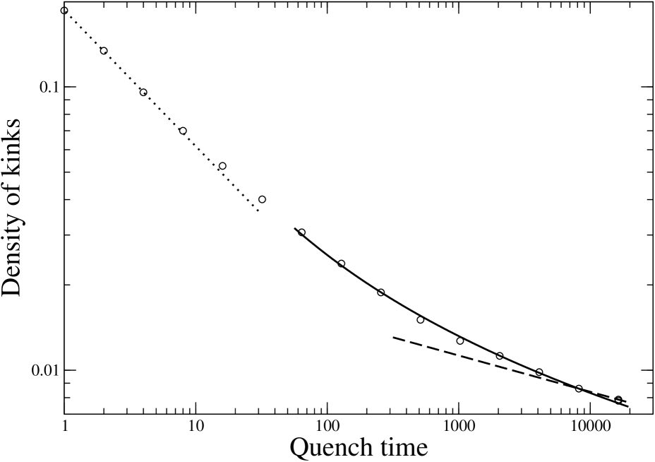
FIG. 2.: Density of kinks $d$ as a function of transition time $\tau_{Q}$ on a lattice of $N=512$ sites. Circles are final kink densities averaged over 4 realizations of $J_{n}$. Error bars set the size of the circles. The solid line is the best fit $d(\tau_{Q})=\frac{0.15}{\hat{\epsilon}^{2}(3.4,\tau_{Q})}$ where $\hat{\epsilon}(\alpha,\tau_{Q})$ is a solution of Eq.(9). The dotted line is the best power law fit $d\sim\tau_{Q}^{-w}$ to the left-most 3 data points and the dashed line is the best power law fit to the right-most 2 data points. The exponents are $w=0.48$ and $w=0.13$ respectively. The exponent $w=0.48$ for the fastest transitions is consistent with the $\frac{1}{2}$ in the pure Ising model.

Conclusion.— This paper is the first test of the Kibble-Zurek mechanism in a disordered system. The test is passed nicely but with an anomalous result that density of defects after a transition depends only logarithmically on the transition rate. Crudely speaking, the density is more or less the same no matter how slow is the transition. This result is in sharp contrast to the standard power law scaling predicted for pure systems. This strongly non-adiabatic behavior can be attributed to the anomalously small energy gap near the critical point which is characteristic for a random system with an infinite disorder fixed point.

Acknowledgements. — I would like to thank Wojciech Zurek for encouragement, and Bogdan Damski for comments on the manuscript. This work was supported in part by ESF COSLAB programme, US Department of Energy, and Polish Government scientific funds (2005-2008) as a research project.

REFERENCES

- [1] S. Sachdev, Quantum Phase Transitions, Cambridge UP 1999.
- [2] T.W.B. Kibble, J. Phys. A 9, 1387 (1976); Phys. Rep. 67, 183 (1980); W.H. Zurek, Nature 317, 505 (1985); Acta Physica Polonica B 24, 1301 (1993); Phys. Rep. 276, 177 (1996).
- [3] P. Laguna and W.H. Zurek, Phys. Rev. Lett. 78, 2519 (1997); A. Yates and W.H. Zurek, ibid. 80, 5477 (1998); N.D. Antunes et al., ibid. 82, 2824 (1999); M.B. Hindmarsh and A. Rajantie, ibid. 85, 4660 (2000); J.R. Anglin and W.H. Zurek, ibid. 83, 1707 (1999).
- [4] V.M.H. Ruutu et al., Nature 382, 334 (1996); C. Baürle et al., ibid. 382, 332 (1996); R. Carmi et al., Phys. Rev. Lett. 84, 4966 (2000); A. Maniv et al., ibid. 91, 197001 (2003); R. Monaco et al., Phys. Rev. Lett. 89, 080603 (2002); Phys. Rev. B 67, 104506 (2003); cond-mat/0503707.
- [5] J. Dziarmaga, Phys.Rev.Lett. 95, 245701 (2005).
- [6] W.H. Zurek et al., Phys. Rev. Lett. 95, 105701 (2005); R.W. Cherng and L.S. Levitov, cond-mat/0512689.
- [7] B. Damski and W.H. Zurek, cond-mat/0511709.
- [8] J. Dziarmaga et al., Phys. Rev. Lett. 88, 167001 (2002); E. Altman and A. Auerbach, Phys. Rev. Lett. 89, 250404 (2002); A. Polkovnikov, Phys. Rev. B. 72, R161201 (2005); F. Cucchietti et al., cond-mat/0601650.
- [9] B. Damski, Phys. Rev. Lett. 95, 035701 (2005).
- [10] R. Shankar and G. Murthy, Phys. Rev. B 36, 536 (1986); B.M. McCoy and T.T. Wu, Phys. Rev. 176, 631 (1968); ibid 188, 982 (1969); R.B. Griffiths, Phys. Rev. Lett. 23, 17 (1969); B.M. McCoy, Phys. Rev. Lett. 23, 383 (1969); Phys. Rev. 188, 1014 (1969).
- [11] D.S. Fisher, Phys. Rev. B 51, 6411 (1995).