A maximum entropy principle explains quasi-stationary states in systems with long-range interactions: the example of the Hamiltonian Mean Field model

Abstract

A generic feature of systems with long-range interactions is the presence of quasi-stationary states with non-Gaussian single particle velocity distributions. For the case of the Hamiltonian Mean Field (HMF) model, we demonstrate that a maximum entropy principle applied to the associated Vlasov equation explains known features of such states for a wide range of initial conditions. We are able to reproduce velocity distribution functions with an analytical expression which is derived from the theory with no adjustable parameters. A normal diffusion of angles is detected and a new dynamical effect, two oscillating clusters surrounded by a halo, is also found and theoretically justified.

Long-range interactions are common in nature Houches02 . Examples include: self gravitating systems Padmanabhan , plasmas Nicholson , dipolar magnets Akhiezer and wave-particle interactions Barre . Theoretical studies have shown that the thermodynamic properties of these systems differ from those of systems with short-range interactions. For instance, long-range interactions may produce a negative microcanonical specific heat LyndenBell68 and, more generally, inequivalence of the canonical and microcanonical ensembles Mukamel . Also the dynamics of models with long-range interactions has been studied, revealing a variety of peculiar features such as the presence of breaking of ergodicity in microcanonical dynamics Celardo ; Schreiber and the existence of quasi-stationary states whose relaxation time to equilibrium diverges with system size antoni-95 ; Taruya . A number of paradigmatic toy models have been proposed that provide the ideal ground for theoretical investigations. Among others, the Hamiltonian Mean Field (HMF) model antoni-95 is nowadays widely analyzed because it displays many features of long range interactions, while being simple to study analytically and numerically. Within the HMF scenario, non-Gaussian velocity distributions Rapisarda and signatures of anomalous diffusion Latora have been reported in the literature. These discoveries have originated an intense debate about the general validity of Boltzmann-Gibbs statistical mechanics for systems with long-range interactions EPN . Non-Gaussian distributions have been fitted using Tsallis’ $q$–exponentials Tsallis , i.e. algebraically decaying profiles predicted within the realm of nonextensive statistical mechanics. Based on these findings, the generalized thermostatistic formulation pioneered by Tsallis was proposed as a tool to describe the properties of quasi-stationary statesRapisarda .

In this Letter, we demonstrate that a maximum entropy principle inspired by Lynden-Bell’s theory of “violent relaxation” for the Vlasov equation allows to explain satisfactorily the numerical simulations performed for the HMF model. Analytically obtained PDF’s are superimposed to the numerics without adjusting any free parameter. In other words, our results point to the fact that there is no need to invoke generalized forms of Boltzmann-Gibbs statistical mechanics to describe the non-equilibrium properties of this system.

The HMF model describes the motion of $N$ coupled rotators and is characterized by the following Hamiltonian

$$H=\frac{1}{2}\sum_{j=1}^{N}p_{j}^{2}+\frac{1}{2N}\sum_{i,j=1}^{N}\left[1-\cos(\theta_{j}-\theta_{i})\right]$$ (1)

where $\theta_{j}$ represents the orientation of the $j$-th rotor and $p_{j}$ is its conjugate momentum. To monitor the evolution of the system, it is customary to introduce the magnetization, a global order parameter defined as $M=|{\mathbf{M}}|=|\sum{\mathbf{m}_{i}}|/N$, where ${\mathbf{m}_{i}}=(\cos\theta_{i},\sin\theta_{i})$ is the local magnetization vector. Starting from out–of–equilibrium initial conditions, the system gets trapped in Quasi-Stationary States (QSS), whose lifetime diverges when increasing the number of particles $N$. Importantly, when performing the mean-field limit ($N\rightarrow\infty$) before the infinite time limit, the system cannot relax towards Boltzmann–Gibbs equilibrium and remains permanently confined in QSS. In this regime, the magnetization is lower than the one predicted by the Boltzmann–Gibbs equilibrium and the system apparently displays a number of intriguing anomalies, e.g. non Gaussian velocity distributions Rapisarda and non standard diffusion in angle Latora . We shall here provide a strong evidence that the above phenomena can be successfully interpreted in the framework of the statistical theory of the Vlasov equation, a general approach originally introduced in the astrophysical and 2D Euler turbulence contexts LyndenBell67 ; Chavanis96 ; PhysAJulien .

First, let us recall that for mean-field Hamiltonians such as (1), it has been rigorously proven BraunHepp that, in the $N\to\infty$ limit, the $N$-particle dynamics is described by the Vlasov equation

$$\frac{\partial f}{\partial t}+p\frac{\partial f}{\partial\theta}-\frac{dV}{d\theta}\frac{\partial f}{\partial p}=0\quad,$$ (2)

where $f(\theta,p,t)$ is the microscopic one-particle distribution function and

$$V(\theta)[f] = 1-M_{x}[f]\cos(\theta)-M_{y}[f]\sin(\theta)~{},$$ (3)

$$M_{x}[f] = \int_{-\pi}^{\pi}\int_{-\infty}^{\infty}f(\theta,p,t)\,\cos{\theta}{\mathrm{d}}\theta{\mathrm{d}}p\quad,$$ (4)

$$M_{y}[f] = \int_{-\pi}^{\pi}\int_{\infty}^{\infty}f(\theta,p,t)\,\sin{\theta}{\mathrm{d}}\theta{\mathrm{d}}p\quad.$$ (5)

The specific energy $h[f]=\int\int(p^{2}/{2})f(\theta,p,t){\mathrm{d}}\theta{\mathrm{d}}p-({M_{x}^{2}+M_{y}^{2}-1})/{2}$ and momentum $P[f]=\int\int pf(\theta,p,t){\mathrm{d}}\theta{\mathrm{d}}p$ functionals are conserved quantities.

We now turn to illustrate the maximum entropy method. The basic idea is to coarse-grain the microscopic one-particle distribution function $f(\theta,p,t)$ into a given set of values. It is then possible to associate an entropy to the coarse-grained distribution $\bar{f}$, i.e. averaged over a box of finite size, and statistical equilibrium can be determined by maximizing this entropy while imposing the conservation of certain Vlasov dynamical invariants. A physical description of this procedure can be found in LyndenBell67 ; Chavanis06 and a rigorous mathematical justification is given in Ref. Michel94 .

In the following, we shall assume that the initial single particle distribution takes only two distinct values, namely $f_{0}=1/(4\Delta_{\theta}\Delta_{p})$, if the angles (velocities) lie within an interval centered around zero and of half-width $\Delta_{\theta}$ ($\Delta_{p}$), and is zero otherwise. This choice corresponds to the so-called “water-bag” distribution which is fully specified by energy $h[f]=e$, momentum $P[f]=\sigma$ and initial magnetization ${\mathbf{M}_{0}}=(M_{x0},M_{y0})$. Vlasov time evolution can modify the shape of the boundary of the “water-bag”, while conserving the area inside it. Hence, the distribution remains two-level ($0,f_{0}$) as time progresses. Coarse-graining amounts to performing a local average of $f$ inside a given box and this procedure results in $\bar{f}$. In this two-level situation, the mixing entropy per particle associated with $\bar{f}$ reads

$$s(\bar{f})=-\int\!\!{\mathrm{d}}p{\mathrm{d}}\theta\,\left[\frac{\bar{f}}{f_{0}}\ln\frac{\bar{f}}{f_{0}}+\left(1-\frac{\bar{f}}{f_{0}}\right)\ln\left(1-\frac{\bar{f}}{f_{0}}\right)\right].$$ (6)

The shape of this entropy derives from a simple combinatorial analysisLyndenBell67 ; Chavanis06 . The maximum entropy principle is then defined by the following constrained variational problem

$$S(e,\sigma)\!=\!\max_{\bar{f}}\biggl{(}\!s(\bar{f})\biggr{|}h(\bar{f})=e;\;\!\!P(\bar{f})=\sigma;\;\!\!\!\int\!\!{\mathrm{d}}\theta{\mathrm{d}}p\bar{f}=1\biggr{)}~{}.$$ (7)

The problem is solved by introducing three Lagrange multipliers $\beta/f_{0}$, $\lambda/f_{0}$ and $\mu/f_{0}$ for energy, momentum and normalization. This leads to the following analytical form of the distribution

$$\bar{f}(\theta,p)=f_{0}\frac{e^{-\beta(p^{2}/2-M_{y}[\bar{f}]\sin\theta-M_{x}[\bar{f}]\cos\theta)-\lambda p-\mu}}{1+e^{-\beta(p^{2}/2-M_{y}[\bar{f}]\sin\theta-M_{x}[\bar{f}]\cos\theta)-\lambda p-\mu}}.$$ (8)

This distribution differs from the Boltzmann-Gibbs one because of the “fermionic” denominator which is originated by the form (6) of the entropy. Inserting expression (8) into the energy, momentum and normalization constraints and using the definition of magnetization, it can be straightforwardly shown that the momentum multiplier $\lambda$ vanishes. Moreover, defining $x=e^{-\mu}$ and ${\mathbf{m}}=(\cos\theta,\sin\theta)$, yields the following system of implicit equations in the unknowns $\beta$, $x$, $M_{x}$ and $M_{y}$

$$f_{0} \frac{x}{\sqrt{\beta}}\int{\mathrm{d}}\theta e^{\beta{\mathbf{M}}\cdot{\mathbf{m}}}F_{0}\left(xe^{\beta{\mathbf{M}}\cdot{\mathbf{m}}}\right)=1$$

$$f_{0} \frac{x}{2\beta^{3/2}}\int{\mathrm{d}}\theta e^{\beta{\mathbf{M}}\cdot{\mathbf{m}}}F_{2}\left(xe^{\beta{\mathbf{M}}\cdot{\mathbf{m}}}\right)=e+\frac{M^{2}-1}{2}$$

$$f_{0} \frac{x}{\sqrt{\beta}}\int{\mathrm{d}}\theta\cos\theta e^{\beta{\mathbf{M}}\cdot{\mathbf{m}}}F_{0}\left(xe^{\beta{\mathbf{M}}\cdot{\mathbf{m}}}\right)=M_{x}$$

$$f_{0} \frac{x}{\sqrt{\beta}}\int{\mathrm{d}}\theta\sin\theta e^{\beta{\mathbf{M}}\cdot{\mathbf{m}}}F_{0}\left(xe^{\beta{\mathbf{M}}\cdot{\mathbf{m}}}\right)=M_{y}$$

with $F_{0}(y)=\int\exp(-v^{2}/2)/(1+y\exp(-v^{2}/2)){\mathrm{d}}v$, $F_{2}(y)=\int v^{2}\exp(-v^{2}/2)/(1+y\exp(-v^{2}/2)){\mathrm{d}}v$, where $v=\sqrt{\beta}p$. This system of equations is then solved using a Newton-Raphson method and the integrals involved are also performed numerically. For $e=\lim_{N\rightarrow\infty}H/N=0.69$, a value often considered in the literature rapisarda , the maximum entropy state has zero magnetization, for any initial magnetization $M_{0}=|{\mathbf{M}_{0}}|<M_{crit}=0.897$. Hence, the QSS distribution does not depend on the angles and the velocity distribution can be simplified into

$$f_{QSS}(p)=f_{0}\frac{e^{-\beta p^{2}/2-\mu}}{1+e^{-\beta p^{2}/2-\mu}},$$ (10)

with $\beta$ and $\mu$ numerically determined from system (A maximum entropy principle explains quasi-stationary states in systems with long-range interactions: the example of the Hamiltonian Mean Field model). Velocity profiles predicted by (10) are displayed in Fig. 1a for different values of the initial magnetization. Gaussian tails are always present, contrary to the power-law ($q$-exponential) fits reported in Ref. Rapisarda . Note that the power-law decay was already excluded on the basis of numerical simulations in Ref. yama for initial zero magnetization states. At $M_{0}=M_{crit}=0.897$, a bifurcation occurs (see Fig. 1b) and the magnetization of the quasi-stationary state $M_{QSS}$ becomes non zero, which means that the equilibrium Lynden-Bell distribution develops an inhomogeneity in angles. The details of this phase transition are further discussed in Ref. pthmf .

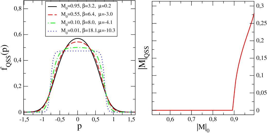
Figure 1: a) Velocity profiles (10) predicted theoretically for different initial magnetizations (see legend, where we have reported also the values of the parameter $\beta$ and $\mu$). b) final magnetization as a function of $M_{0}$. A phase transition is observed at $M_{0}=0.897$ for $e=0.69$.

We validate our theoretical findings in the initial magnetization range $M_{0}\in[0,M_{crit}]$, by performing numerical simulations with $N$ ranging from $10^{3}$ to $10^{7}$. Numerical velocity distributions are compared in Fig. 2 with the analytical solution (10). Although not a single free parameter is used, we find an excellent agreement in the tails of the distribution. The discrepancies observed in the center of the distributions are commented below.

To discuss the behavior of $M$ in the QSS, one must distinguish different magnetization intervals. Consider first the interval $M_{0}\in[M_{a},M_{crit}]$, with $M_{a}\approx 0.5$. Both $M_{x}$ and $M_{y}$ are found to approach zero when the number of rotators is increased, in agreement with the theory outlined above. Our results correlate well with the scaling $|M|\propto N^{-1/6}$ reported in Ref. rapisarda . Numerical simulations also confirm the presence of a bifurcation at $M_{0}=M_{crit}$, and indicate that the distribution in angles is indeed inhomogeneous above this value. Interestingly, when the initial magnetization lies instead in the interval $[0,M_{a}]$, $M_{x}$ and $M_{y}$ display regular oscillations in time, which appear only when a large enough number of rotators ($N>10^{6}$) is simulated. It is important to emphasize that the oscillations are centered around zero, i.e. the equilibrium value predicted by our theory.

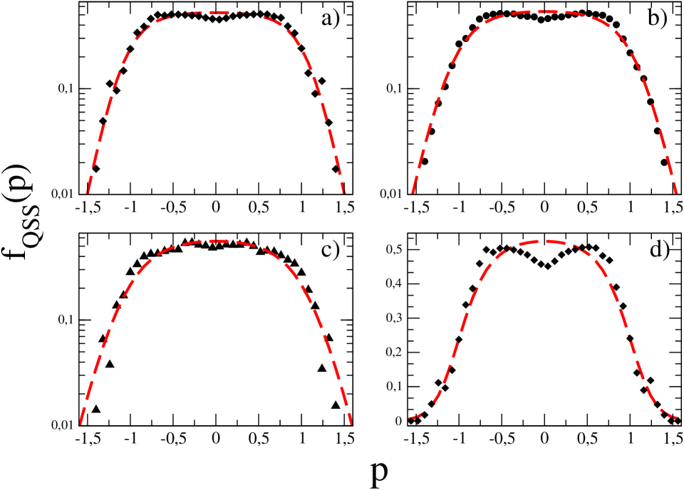
Figure 2: Velocity distribution functions. Symbols refer to numerical simulations, while dashed lines stand for the theoretical profile (10). Panels a), b) and c) present the three cases ${M_{0}}=0.3$, ${M_{0}}=0.5$ and ${M_{0}}=0.7$ in lin-log scale, while panel d) shows the case ${M_{0}}=0.3$ in lin-lin scale. The numerical curves are computed from one single realization with $N=10^{7}$ at time $t=100$. Here $e=0.69$.

We now discuss the presence of two symmetric bumps in the velocity distributions obtained numerically (see Fig. 2). This is a consequence of a collective phenomenon which leads to the formation of two clusters in the $(\theta,p)$ plane. Both clusters form early in time and then acquire constant opposite velocities which are maintained during the time evolution, thus enlarging their relative separation. Consequently, the bumps displayed by the velocity distributions are not transient features, but represent instead an intrinsic peculiarity of QSS. To the best of our knowledge, this is a new collective phenomenon which has not been previously detected. A simple dynamical argument can be elaborated to shed light onto the process of formation of the clusters. Consider the one-particle Hamiltonian $\epsilon(\theta,p)=\frac{p^{2}}{2}-M_{x}\cos\theta-M_{y}\sin\theta$ associated to (1), where $(\theta,p)$ are the conjugate variables of the selected rotor. For short times, $\theta\sim\theta_{0}+p_{0}t$. One then finds $M_{x}\simeq(\sin{\Delta_{\theta}}\sin{\Delta_{p}t})/(\Delta_{\theta}\Delta_{p}t)$ and $M_{y}\simeq 0$. Using this result, one ends up with

$$\epsilon(\theta,p)=\frac{p^{2}}{2}+\frac{\sin{\Delta_{\theta}}}{2\Delta_{\theta}\Delta_{p}t}\left[\sin\left(\theta-\Delta_{p}t\right)+\sin\left(\theta+\Delta_{p}t\right)\right]~{},$$

which corresponds to the Hamiltonian of one particle interacting with two waves of phase velocities $\pm\Delta_{p}$. Depending on the initial condition, the particles can be trapped in one of the two resonances, the latter being therefore directly responsible for the arising of two highly populated regions. Moreover, by including higher order corrections to the above calculation one can show that the two resonances tend to overlap when $M_{0}\rightarrow 1$, in agreement with our numerical findings.

Having derived an analytical expression for the velocity distribution function (10), which is fully validated by the numerics, enables to take advantage of the predictions recently obtained in Ref. BouchetDauxois , where it has been demonstrated that momentum autocorrelation functions can be deduced by knowing only the tails of the velocity distributions. Since these are Gaussian (see Eq. (10)), one expects algebraic decay of momentum autocorrelation. The mean square displacement of the angles $\sigma^{2}(t)=\frac{1}{N}\sum_{i}{[\theta_{i}(t)-\theta_{i}(0)]^{2}}$ is also a quantity of interest. The scaling $\sigma^{2}\propto t^{\gamma}$ defines the diffusive behavior: $\gamma=1$ corresponds to normal diffusion and $\gamma=2$ to free particle ballistic dynamics. Intermediate cases correspond to the anomalous diffusion behavior. Here, for all water-bag initial conditions, the behavior of the momentum autocorrelation function implies BouchetDauxois that a weakly anomalous diffusion has to be expected, with a diffusion exponent $\gamma=1$ and logarithmic corrections.

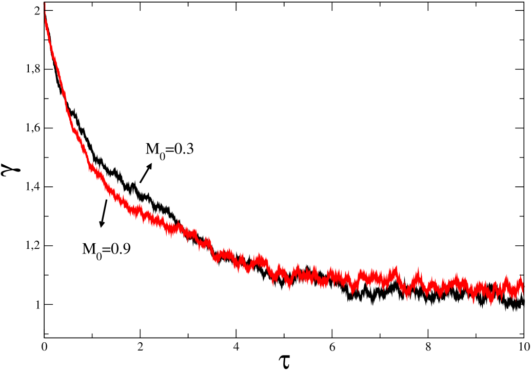
Figure 3: The exponent $\gamma={\rm d}\log(\sigma^{2})/{\rm d}\log(t)$ is plotted as a function of the rescaled time $\tau=t/N$. Starting from the initial ballistic value $2$, it converges to the normal diffusion exponent $1$. Simulations refer to $M_{0}=0.3$, and $M_{0}=0.9$. Here $N=10^{5}$ and $e=0.69$.

On the numerical simulations side, it is claimed in Ref. rapisarda that the QSS display anomalous diffusion with an exponent $\gamma$ in the range $1.4-1.5$ for $0.4\leq M_{0}\leq 1$. These results are contradicted by more recent papers yama1 , where normal diffusion behavior is found. To provide further insight, we have monitored the time evolution of $\sigma^{2}$ by employing a larger number of particles than in previous investigations. As clearly demonstrated by the inspection of Fig. 3, a large value of the exponent $\gamma$ is clearly excluded. On the contrary, the almost normal diffusion found is in complete agreement with the theoretical scenario discussed above.

In this paper, by drawing analogies with the statistical theory of “violent relaxation” in astrophysics and 2D Euler turbulence, we have analytically derived known properties of the quasi-stationary states of the HMF model. In particular: $i)$ velocity probability distributions in all quasi-stationary states investigated are well described by Lynden-Bell statistics (10); $ii)$ Gaussian tails of such maximum entropy states ensure an algebraic decay of momentum autocorrelation functions and, hence, a normal diffusion of the angles. Our theoretical approach is fully predictive, contrary to results obtained using nonextensive thermostatisticsTsallis , which consist in parametric fits that are not justified from first principlesRapisarda . Despite this success of “violent relaxation” theory, we do not expect it to be so precise in all long-range systems: due to incomplete relaxation of the Vlasov equation LyndenBell67 ; Chavanis96 ; Chavanis06 , the QSS should deviate somewhat from Lynden-Bell’s statistical prediction. Besides that, we have discovered that a double cluster spontaneously forms for all magnetizations. This collective effect was not known before. Similar time-dependent quasi-stationary states have been recently found in Ref Kaneko . Our maximum entropy principle is unable to capture this phenomenon, for which we have developed an analytical approach based on analogies with similar effects encountered in plasma-wave Hamiltonian dynamics. More refined maximum entropy schemes, accounting for the conservation of additional invariants besides the normalization, are expected to give a full description of these phenomena and represent a challenge for future investigations.

We acknowledge financial support from the PRIN05-MIUR project Dynamics and thermodynamics of systems with long-range interactions.

References

- (1) T. Dauxois, S. Ruffo, E. Arimondo, M. Wilkens, Dynamics and Thermodynamics of Systems with Long Range Interactions, Lect. Not. Phys. 602, Springer (2002).
- (2) T. Padmanabhan, Phys. Rep. 188, 285 (1990)
- (3) D. R. Nicholson, Introduction to plasma physics Krieger Publishing Company, Malabar, Florida (1992)
- (4) L. Q. English, M. Sato and A. J. Sievers, Phys. Rev. B 67 024403 (2003).
- (5) J. Barré et al., Phys. Rev E 69, 045501(R) (2004).
- (6) D. Lynden-Bell and R. Wood, Mon. Not. R. Astron. Soc. 138, 495 (1968).
- (7) J. Barré et al., Phys. Rev. Lett. 87, 030601 (2001).
- (8) F. Borgonovi et al, J. Stat. Phys. 116, 235 (2004).
- (9) D. Mukamel et al , Phys. Rev. Lett., 95, 240604 (2005).
- (10) M. Antoni and S. Ruffo, Phys. Rev. E 52, 2361 (1995).
- (11) A. Taruya and M. Sakagami, Phys. Rev. Lett. 90, 181101 (2003).
- (12) V. Latora, A. Rapisarda and C. Tsallis, Phys. Rev. E 64, 056134 (2001).
- (13) V. Latora, A. Rapisarda and S. Ruffo, Phys. Rev. Lett. 83, 2104 (1999).
- (14) J. P. Boon and C. Tsallis (Eds.), Europhysics News, 36 (2005).
- (15) C. Tsallis, J. Stat. Phys. 52, 479 (1988).
- (16) J. Barré et al., Physica A 365, 177 (2006)
- (17) D. Lynden-Bell, Mon. Not. R. Astron. Soc. 136, 101 (1967).
- (18) P. H. Chavanis et al, Astrophys. J. 471, 385 (1996); P. H. Chavanis, Physica A 365, 102 (2006).
- (19) W. Braun and K. Hepp, Comm. Math. Phys. 56, 101 (1977).
- (20) P. H. Chavanis, Physica A 359, 177 (2006).
- (21) J. Michel and R. Robert, Comm. Math. Phys. 159, 195 (1994).
- (22) Y. Y. Yamaguchi et al, Physica A 337, 36-66 (2004).
- (23) P. H. Chavanis, [cond-mat/0604234].
- (24) A. Pluchino, V. Latora and A. Rapisarda, Phys. Rev. E 69, 056113 (2004).
- (25) F. Bouchet and T. Dauxois, Phys. Rev. E 72, 045103(R) (2005).
- (26) Y. Y. Yamaguchi, Phys. Rev. E 68 066210 (2003); L. G. Moyano and C. Anteneodo, Phys. Rev. E 74, 1 (2006).
- (27) H. Morita and K. Kaneko, Phys. Rev. Let. 96 050602 (2006).