Geometric and impurity effects on quantum rings in magnetic fields

Abstract

We investigate the effects of impurities and changing ring geometry on the energetics of quantum rings under different magnetic field strengths. We show that as the magnetic field and/or the electron number are/is increased, both the quasiperiodic Aharonov-Bohm oscillations and various magnetic phases become insensitive to whether the ring is circular or square in shape. This is in qualitative agreement with experiments. However, we also find that the Aharonov-Bohm oscillation can be greatly phase-shifted by only a few impurities and can be completely obliterated by a high level of impurity density. In the many-electron calculations we use a recently developed fourth-order imaginary time projection algorithm that can exactly compute the density matrix of a free-electron in a uniform magnetic field.

I Introduction

The possibilities of utilizing the Aharonov-Bohm (AB) effect in future nanotechnology has stimulated significant recent progress in fabricating nanoscopic quantum rings. lorke ; fuhrer ; keyser Since the capabilities to control the electron number in the ring and to modify its geometry are essential for observing and exploiting new phenomena, systems with these capabilities have attracted much theoretical interest.

Lorke and co-workers lorke have applied self-assembly techniques to create InGaAs and GaAlAs/GaAs rings containing only a few electrons. The weak electron-electron interaction in these rings makes them most suitable for optical experiments, and the observed state transitions can be well explained with the single-electron spectrum of a parabolic ring. pekka On the other hand, Keyser and co-workers keyser have reached the strongly correlated regime by omitting the screening gate on top of a few-electron quantum ring fabricated from a GaAs/AlGaAs heterostructure. They were able to observe fractional AB oscillations with a period of $\Phi_{0}/N$, where $\Phi_{0}=h/e$ is the flux quantum and $N$ is the electron number. Exact diagonalization of a few-electron Hamiltonian niemela has shown that the electron-electron interactions break the degeneracy between the singlet and triplet states, leading to fractional oscillations. Similar results have been obtained within the Heisenberg model deo and also by recent Monte Carlo calculations. emperadornew Both have clarified the role of the electron localization in the fractional AB effect. The role of the (two-dimensional) width of the ring is, however, still unclear in the strong-interaction limit.

From magnetotransport experiments in the Coulomb blockade regime one can infer the discrete energy levels of a quantum ring. fuhrer Moreover, these measurements have been performed for both circular and square ring-geometries; the latter corresponds to a chaotic Sinai billiard, kaaos i.e., a circular antidot at the center of a square quantum dot. In such a symmetry-broken quantum ring, the increasing magnetic field induces regularity in the amplitude and position of the Coulomb peaks. These dots have been estimated to contain hundreds of electrons. The interactions were screened by a top gate, hence the simple single-electron picture provides a sufficient description of the spectrum. fuhrer

We examine in this paper the energetics of circular, square-shaped, and impurity-doped two-dimensional (2D) quantum rings containing up to $N\sim 20$ strongly interacting electrons. We shall focus on the measurable quantities such as the chemical potentials, addition energies, and the magnetization. We will identify the quasiperiodic AB oscillations as well as different magnetic phases, and find, in agreement with the experiments, fuhrer that these become very similar between circular and square rings at large $N$ and in high magnetic fields. In these phases we find similarities to integer and fractional quantum Hall states of quantum dots. oosterkamp ; henri We also carry out a statistical analysis of the addition-energies for quantum rings containing randomly distributed Coulombic impurities. Increasing the number of impurities leads to a systematic phase shift in the AB oscillations. As a result of the electron-electron interactions, the high-disorder limit is characterized by a Gaussian-like addition-energy distribution. This shape indicates the disappearance of the AB oscillations.

In this work, we solve the many-electron problem in a strong, uniform magnetic field by use of the spin-density-functional theory (SDFT). To solve the Kohn-Sham (KS) equations for thousands of impurity configurations, we use our recently developed fourth-order projection algorithm magalg to determine the occupied KS orbitals. This algorithm is highly efficient, since the number of Fast Fourier Transforms used for solving the KS spectrum remains the same even in the presence of a magnetic field. This is because at its core, our algorithm is capable of exactly computing the density matrix of a free electron in an arbitrarily strong magnetic field. Thus unlike other methods of solving the Schrödinger equation, the magnetic field part of the physics is hardwired into our algorithm. Also, instead of the usual slow-convergent, charge-mixing iterations, we update the charge densities by our linear-response algorithmcluster with accelerated Newton-Raphson convergence. These significant algorithmic advances are not based incremental improvement of numerical methods, but in attuning to the fundamental physics of the problem. The details of the algorithms are presented in the Appendix.

II Quantum-ring model

We focus on quantum rings realized in semiconductor heterostructures, which can be modeled by localizing electrons to a 2D (xy) plane. We use the effective-mass approximation with GaAs parameters, i.e., the effective electron mass $m^{*}=0.067\,m_{e}$ and the dielectric constant $\kappa=12.7$. The many-electron Hamiltonian is written in SI units as

$$H = \frac{1}{2m^{*}}\sum^{N}_{i=1}\left[-i\hbar\nabla_{i}+e\mathbf{A}({\mathbf{r}}_{i})\right]^{2}+\sum^{N}_{i<j}\frac{e^{2}}{4\pi\epsilon_{0}\kappa|{\mathbf{r}}_{i}-{\mathbf{r}}_{j}|}$$ (1)

$$+ \sum^{N}_{i=1}\left[V_{\rm ext}(r_{i},\theta_{i})+V_{\rm imp}({\mathbf{r}}_{i})+g^{*}\mu_{B}Bs_{z,i}\right].$$

The magnetic field ${\mathbf{B}}=B\hat{z}$ is chosen perpendicular to the xy plane, the vector potential is then, in linear gauge, $\mathbf{A}=-By\,\mathbf{e}_{x}$. The last term is the Zeeman energy that couples the external magnetic field with the electron spin. Here $g^{*}=-0.44$ is the effective gyromagnetic ratio, $\mu_{B}=e\hbar/2m_{e}$ is the Bohr magneton, and $s_{z}=\pm\frac{1}{2}$ for the up and down spins, respectively. The spin-orbit interaction is expected to be negligible in the GaAs structure having a wide band gap, it is therefore ignored in the Hamiltonian. The external potential that confines the electrons and defines the geometry of the quantum ring is chosen, in polar coordinates, to be

$$V_{\rm ext}(r,\theta)=\frac{1}{2}m^{*}\omega_{0}^{2}r^{2}\left[1+\alpha\cos(p\,\theta)\right]+V_{0}e^{-r^{2}/d^{2}},$$ (2)

where $\hbar\omega_{0}=5$ meV is the confinement strength, and the cosine term defines the confinement geometry. We apply a circular and square shape determined by $\alpha=0$ and $(\alpha,p)=(0.2,4)$, respectively. serra The Gaussian term in Eq. 2 defines an antidot at the center, thus producing a ring-like shape of our system. We set $V_{0}=200$ meV and the width parameter $d=10$ nm, which is a sufficient value for two-dimensionality. The shapes of the total external potentials for the both geometries are shown in Fig. 1.

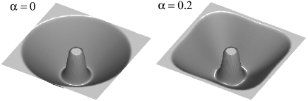
Figure 1: Shapes of the external confinement potentials determining circular and square quantum rings with $\alpha=0$ and $0.2$ in Eq. 2, respectively.

Within the circular ring geometry ($\alpha=0$), we also apply an impurity potential describing repulsive Coulombic impurities located randomly in the vicinity of the quantum-ring system. It is written as

$$V_{\rm imp}({\mathbf{r}})=\sum^{N_{\rm imp}}_{k=1}\frac{-e}{4\pi\epsilon_{0}\kappa\sqrt{({\mathbf{r}}-{\mathbf{R}}_{k})^{2}+d^{2}_{k}}},$$ (3)

where $N_{\rm imp}$ is the number of impurities, and ${\mathbf{R}}_{k}$ and $d_{k}$ are their random lateral and vertical positions in the ranges of $0\leq R_{k}\leq 100\,{\rm nm}$ and $0\leq d_{k}\leq 10\,{\rm nm}$, respectively. This model, motivated by single-electron tunneling experiments, jens has been applied recently in statistical studies on quantum dots. michael1 ; michael2 Similarly to those studies, for each $N_{\rm imp}=5\ldots 30$ we apply $1000$ spatial configurations in order to obtain good statistics.

III Single-electron spectra

In order to obtain insight into the energy-level structure in the quantum rings studied, we first computed the single-electron spectra of a system of noninteracting electrons as a function of the magnetic-field strength. Figure 2

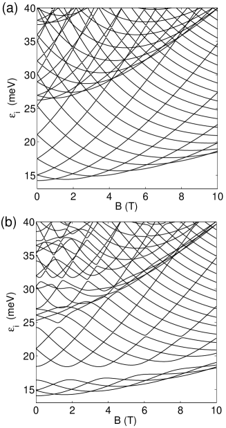
Figure 2: Single-electron spectra in circular (a) and square (b) quantum rings as a function of the magnetic field. The Zeeman splitting is omitted.

shows the eigenenergies $\epsilon_{i}$ for a circular (a) and square (b) quantum ring with up to $i\sim 25$ and $B=10$ T. The spectrum of our circular ring is similar to the one obtained using a pure parabolic 2D ring model. pekka Due to the finite ring width, the second Fock-Darwin level and the beginning of the third one can be seen in the spectrum. Increasing the width by making $d$ smaller brings the upper Landau levels lower in energy.

In the spectrum of a square ring shown in Fig. 2(b), the four lowest energy levels are decoupled from the upper levels and form a braid-like structure as a function of the magnetic field. Similar decoupling can be observed for the next four levels at low fields. This behavior results from the four-fold symmetry of the square confining potential. The probability densities of the lowest eigenstates show that the four lowest levels correspond to energetically stable corner modes. The next four levels in the lower row, instead, correspond to the side modes. Valín-Rodríquez and co-workers serra have analyzed modes of this type in their far-infrared-absorption studies on triangular and square quantum dots.

In addition to the decoupled single-electron levels, there are several other avoided level crossings in the spectrum of a square ring, particularly at low magnetic fields. The level repulsion in quantum dots is usually interpreted as a signature of quantum chaos. kaaos Contrary to the square quantum dot, esaphysica our square-ring system is non-integrable also at zero magnetic field. A similar system having steep walls (Sinai billiard) is a famous example of a chaotic system, it has been extensively studied in the context of both classical and quantum billiards. kaaos In Fig. 2(b) it can be seen that the number of avoided crossings decreases at high magnetic fields because the electron orbitals shrink due to the increasing magnetic confinement. However, the system remains chaotic, again in contrast with a square quantum dot which becomes integrable at $B\rightarrow\infty$.

The presence of external impurities (see Eq. 3) lead to irregular deviations in the single-electron energy levels. In Fig. 3

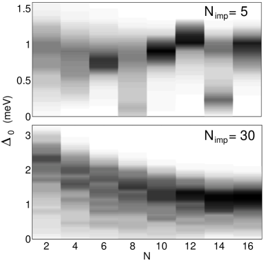
Figure 3: Level-spacing distributions of noninteracting electrons at $B=10$ T in impurity-affected quantum rings. The level spacings are calculated from one thousand random impurity configurations for $5$ (upper panel) and $30$ impurities (lower panel).

we plot distributions (gray scale) of single-electron level spacings at $B=10$ T calculated from one thousand random impurity configurations for $N_{\rm imp}=5$ and $30$, respectively. The level spacings correspond to the addition energies of noninteracting electrons defined as $\Delta_{0}(N)=\epsilon_{N/2+1}-\epsilon_{N/2}$. In the case of five impurities the distributions are approximately peaked around the level spacings of the clean quantum ring (cf. Fig. 2 at $B=10$ T). However, when $N=14$ ($\epsilon_{8}-\epsilon_{7}$), for example, there are two maxima in the distribution as seen in the upper panel of Fig. 3. These result from the fact that while these two states are nearly degenerate at that field, they have a different slope with respect to $B$. Hence, in strongly disordered configurations the level splitting is considerably larger than in the approximately clean cases, leading to a two-peak structure. When the number of impurities is increased to 30 (lower panel in Fig. 2), the signatures of the shell structure clearly disappear. On a coarse scale, the distributions resemble Wigner-Dyson forms indicating a disordered system. However, the distributions show fine structure resulting from the correlation between consecutive energy levels in the presence of a high number of impurities.

IV Many-electron properties

IV.1 Circular and square geometries

For the corresponding many-electron problem we apply the SDFT. Using the numerical scheme outlined in the Appendix, we have calculated the total energies of different spin states for $N=1\ldots 17$ and for each magnetic-field strength up to $10$ T in steps of $0.2$ T. The ground state for each $N$ is then defined as the spin state having the lowest energy $E(N)$. Figure 4

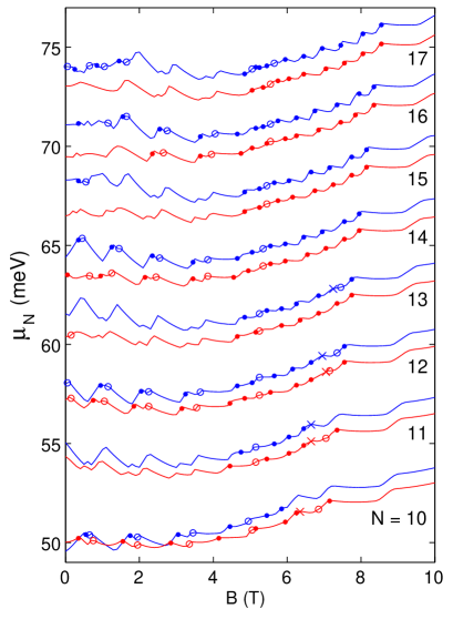
Figure 4: (color online). Chemical potentials for $N=10\ldots 17$ in circular (upper blue lines) and square (lower red lines) quantum rings. The filled circles, open circles, and crosses correspond to the spin changes $S\rightarrow S+1$, $S\rightarrow S-1$, and $S\rightarrow S+2$, respectively.

shows the chemical potentials $\mu(N)=E(N)-E(N-1)$ for $N=10\ldots 17$ in circular (upper blue lines) and square (lower red lines) quantum rings. We omit the low electron numbers in Fig. 4 to display the differences between two rings more clearly. The transitions in the ground-state spins are marked in Fig. 4 such that the filled circles denote an increase $S\rightarrow S+1$, and the open circles mark a decrease $S\rightarrow S-1$. The crosses mark an increase of $S\rightarrow S+2$. The rightmost points correspond to full spin polarization. The chemical potentials for $N=10,11$ and $12$ in circular ring agree with those of Emperador and co-workers. emperador The trend of pairing between peaks for consecutive values of $N$, as well as quasiperiodic oscillations analyzed in Ref. emperador, , are found to continue up to higher electron numbers. We see the predicted violations in the pairing, e.g., at $B\sim 1$ and $2.2$ T when $N=11-12$. These are explained by Hund’s rule, causing partial spin polarization near the level crossings in the corresponding single-electron spectrum (see Fig. 2).

As seen in Fig. 4, the evolution of $\mu(N)$ as a function of $B$ is qualitatively similar in circular and square rings, although the oscillations at low fields are considerably stronger in the circular case. This difference is due to the level repulsion of the square-shaped ring that leads to smoother behavior of the total energies. The tendency of the symmetry-breaking to even out the oscillations has been detected also in quantum dots containing external impurities. jens ; gycly The square ring shows also increased stability as a small increase in $\mu(N)$ when $N=4$ or $8$ [not plotted in Fig. 4]. This effect is presented and discussed in detail in connection with the addition energies below.

The chemical potentials could be directly compared to Coulomb blockade oscillations of transport measurements, but we are not aware of such experiments for quantum rings. In the quantum dots, however, a remarkably good agreement has been obtained between the experimental result of the Coulomb blockade oscillations oosterkamp and SDFT calculations. henri

Next we consider the second energy differences, i.e., the addition energies defined as $\Delta(N)=\mu(N+1)-\mu(N)=E(N-1)-2E(N)+E(N+1)$. Besides chemical potentials, they are also measurable quantities, fuhrer and give a more detailed view on the energetic structure of quantum rings. Figure 5

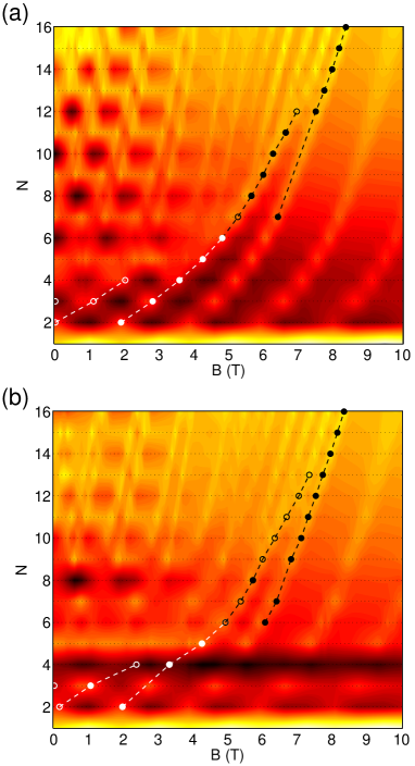
Figure 5: (color online). Addition energies (yellow: low, black: high) as a function of the magnetic field and up to 16 electrons in circular (a) and square (b) quantum rings. The open and filled circles mark the first and final full spin polarizations, respectively. The dashed lines are plotted to guide the eye.

shows the full phase diagram of $\Delta(N)$ as a function of $B$ and $N$ for a circular (a) and square (b) ring. The light and dark regions correspond to low and high addition energies, respectively. The open and filled circles mark the first and final full spin polarizations, and the dashed lines are to guide the eye. The characteristic energy oscillations are evident in both geometries. The structure of the oscillations, however, shows interesting differences. In the circular case there are three easily distinguished phases: (i) strong oscillations at low $B$ that mostly correspond to spin changes $0\rightarrow 1\rightarrow 0$ following Hund’s rule; (ii) spin flip region at intermediate $B$ that becomes broader as $N$ increases; and (iii) a polarized regime in high magnetic fields on the right side of the dashed line(s), characterized by large-width oscillations of a period $\Delta\Phi\sim\Phi_{0}$ (the flux $\Phi=BA$, where $A$ is the estimated ring area). A similar division can be found in the addition energies of a square ring [Fig. 5(b)]. However, the effect of the four-fold asymmetry is clear in the pronounced stability of the four-electron ring. It results from the decoupling of the lowest single-electron levels shown in Fig. 2. The stability is strongest after the polarization at $B\sim 3\ldots 4$ T, since then all the four separated levels are (singly) occupied. Likewise, the eight-electron ring is particularly stable at low fields when $S=0$.

The addition energies in high magnetic fields are very similar between the circular and square rings, particularly when $N$ is large. This result agrees qualitatively with the experimental observation of Fuhrer and co-workers. fuhrer It can be explained by the fact that the magnetic confinement has a parabolic shape. Furthermore, the electron-electron interactions make the square ring effectively more symmetric. jens In the onset of the full spin polarization there are two differences. First, the square ring has a kink at $N=4$ due to its specific energy spectrum discussed in Sec. III. Secondly, there are many depolarizations in the square ring when $N=6\ldots 13$, occurring between the first and second full spin polarizations marked as open and solid circles in Fig. 5, respectively. However, this effect is relatively faint and its emergence is very sensitive to the ring parameters. For example, depolarization can be obtained in the circular ring at $N=8\ldots 11$ if the Zeeman energy in Eq. 1 is slightly reduced.

The different magnetic phases discussed above can be characterized in detail from the magnetization curves for large electron numbers. The magnetization is defined as the derivative of the free energy with respect to the magnetic field and reduces in zero temperature to $M=-\partial{E_{\rm tot}}/\partial{B}$. In Fig. 6

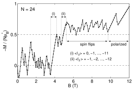
Figure 6: Magnetization of a 24-electron circular quantum ring. Different magnetic phases characteristic of finite Fermion systems are marked in the figure.

we plot the magnetization of a 24-electron circular quantum ring as a function of the magnetic field strength $B$. In the two steps marked in the figure as (i) and (ii), the ground-state spin is zero and the (doubly) filled angular-momentum states are $\left<l_{z}\right>=0,-1,\ldots,-11$ and $-1,-2,\ldots,-12$, respectively. They are calculated as the expectation values of the angular momentum operator $\hat{l}_{z}=-i\hbar[x(\partial/\partial{y})-y(\partial/\partial{x})]$ for different KS states. The first occupation (i) from $\left<l_{z}\right>=0$ to $-(N/2-1)$ directly corresponds to a quantum Hall state qhkirja with a filling factor $\nu=2$. In the spin-flip region at $B\sim 5\ldots 10$ T the spin polarization of the ring gradually increases and the magnetization is characterized by short-period oscillations. In the first fully polarized $(S=12)$ state the occupation is $\left<l_{z}\right>=-2,-3,\ldots,-25$. After that the oscillations become regular such that each step corresponds to an increase of 24 in the total angular momentum $|L_{z}|=\sum_{i}{|\left<l^{i}_{z}\right>}|$, as the electrons jump from $\left<l^{i}_{z}\right>$ to $\left<l^{i}_{z}\right>-1$. Consequently, the hole in the electron density at the center of the ring increases, and there are no signs of edge reconstruction, which confirms the result of Emperador and co-workers. empr

The behavior in the electron occupations and magnetization as a function of $B$ is similar to that of a quantum-dot system. henri The most obvious difference is that the $\nu=1$ state with an occupation from $\left<l_{z}\right>=0$ to $-(N-1)$ is not found in quantum rings. This state, i.e., the maximum-density droplet, macdonald is particularly stable in quantum dots and has been observed experimentally. oosterkamp However, we expect that in quantum rings the signatures of the $\nu=2$ state and spin flips, as well as the regular oscillations in the polarized ($\nu<1$) regime could be observed in magnetization experiments using, for example, sensitive micromechanical magnetometers. schwarz

IV.2 Impurity effects

Finally we analyze the effect of impurities on the addition energies in a many-electron system. The applied impurity model is defined in Eq. 3. For simplicity, we focus here on the fully spin-polarized regime where the addition-energy oscillations in corresponding impurity-free quantum rings (see Fig. 5) are regular. Figure 7

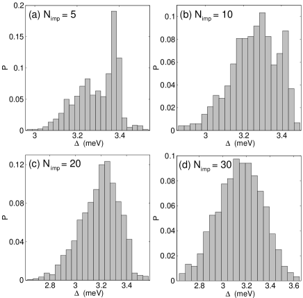
Figure 7: Addition-energy distributions of a 12-electron quantum ring having 5 (a), 10 (b), 20 (c), and 30 (d) impurities. The magnetic field is set to $B=10$ T corresponding to the fully-polarized regime.

shows the addition-energy distributions of a 12-electron quantum ring at $B=10$ T. For each number of impurities we have calculated the electronic structure and energetics for one thousand random impurity configurations. We find that the distribution for $N_{\rm imp}=5$ shows a clear two-peak structure. This is due to the fact that in this case the rings can be roughly divided into relatively disordered and clean ones depending on the actual location of the impurities. These two types of rings have then different radii on the average, which eventually leads to a phase shift in the AB oscillations as a function of the magnetic field.

As the number of impurities is increased, the two peaks gradually merge and finally at $N_{\rm imp}=30$, corresponding to an impurity density of $\sim 10^{-3}{\rm nm}^{-1}$, we find a Gaussian-like symmetric distribution shown in Fig. 7(d). The symmetric shape is a result of the electron-electron interactions that even out the tilted shape and irregularities found in the level-spacing distributions (noninteracting electrons) shown in Fig. 3. The Gaussian shape is qualitatively similar to what has been found in disordered quantum dots both experimentally sivan ; patel and theoretically using Hartree-Fock cohen and density-functional methods. hirose ; jiang ; michael2 In addition, modifications to the random matrix theory that take the interactions into account have led to a good agreement between the experiments and the theory, alhassid whereas the bare random matrix theory yields the Wigner-dyson distribution. Hence, we expect that the distribution shown in Fig. 7(d) for quantum rings corresponds to the limit of disorder which ultimately indicates the disappearance of the AB oscillations. Following the analogy to quantum-dot systems, jiang we expect that a Gaussian-like distribution could be obtained in conductance experiments for large ($N>100$) quantum rings. In that case the addition-energy statistics would be determined as a function of $N$.

V Summary

We have used efficient computational algorithms for solving the Kohn-Sham equations of spin-density-functional theory to examine the effects of geometric deviations on the ground-state properties of two-dimensional quantum rings in magnetic fields. Due to the circular shape of the magnetic confinement, increasing magnetic field evens out the variations between the energetics of quantum rings of different geometries. The measurable quantities in both systems can be characterized by quasiperiodic oscillations, of which we have been able to identify the quantum-ring counterparts of the integer quantum-Hall states. However, the Aharonov-Bohm oscillations at high fields are very sensitive to the presence of external impurities which may produce a systematic phase shift. In the high-impurity (disorder) limit the electron-electron interactions make the addition-energy distributions Gaussian-like. This behavior, indicating the disappearance of the oscillations, is similar to what has been found in quantum dots.

*

Appendix A Numerical scheme

Our numerical procedure for solving the electronic properties of the system within the SDFT consists of two parts, namely, the solution of an effective Schrödinger equation [the Kohn-Sham (KS) equation] and the self-consistent determination of the spin-densities. The KS equation in a magnetic field is

$$\left[\frac{1}{2m^{\star}}(-i\hbar\nabla+e\mathbf{A}(\mathbf{r}))^{2}+V_{\rm KS}({\mathbf{r}})\right]\Phi_{i}^{\sigma}(\mathbf{r})=\epsilon_{i}\Phi_{i}^{\sigma}(\mathbf{r}),$$ (4)

where the KS potential $V_{\rm KS}(\mathbf{r})$ is a sum of the external potential defined above, the Hartree potential, and the exchange-correlation potential given as $V_{\rm xc}({\mathbf{r}})=\delta{E_{\rm xc}}[\rho,\xi]/\delta\rho^{\sigma}{({\mathbf{r}})}$. Here $\rho^{\sigma}$ are the electron spin densities, $\sigma$ denotes the spin index, and $\xi(\mathbf{r})=[\rho^{\uparrow}(\mathbf{r})-\rho^{\downarrow}(\mathbf{r})]/\rho(\mathbf{r})$ is the local spin polarization. For $E_{\rm xc}$ we use the local spin-density approximation with the functional provided by Attaccalite and co-workers. AMGB02

The lowest $n$ solutions of the eigenvalue problem (4) are obtained by applying the evolution operator,

$$\mathcal{T}(\epsilon)\equiv\text{e}^{-\epsilon H}$$ (5)

repeatedly to a set of states $\{\psi_{j},\,1\leq j\leq n\}$, and orthogonalizing the states after every step. Instead of the commonly used second-order factorization in combination with the Gram-Schmidt orthogonalization, we use the fourth-order factorization for the evolution operator given by Suzuki96 ; ChinPLA97

$$\mathcal{T}^{(4)}(\epsilon)=e^{-\frac{1}{6}\epsilon V}e^{-\frac{1}{2}\epsilon T}e^{-\frac{2}{3}\epsilon\widetilde{V}}e^{-\frac{1}{2}\epsilon T}e^{-\frac{1}{6}\epsilon V}+\mathcal{O}(\epsilon^{5})\,,$$ (6)

where

$$T=\frac{1}{2m^{\star}}\mathbf{\Pi}^{2}\equiv\frac{1}{2m^{\star}}\left[\Pi_{x}^{2}+\Pi_{y}^{2}\right],\quad\mathbf{\Pi}={\bf p}+e{\bf A}(\mathbf{r})$$ (7)

is the kinetic-energy operator. We have defined the local modified potential Suzuki96 ; ChinPLA97 as

$$\widetilde{V}=V+\frac{1}{48}\epsilon^{2}[V,[T,V]].$$ (8)

Note that the vector potential ${\bf A}(\mathbf{r})$ does not contribute to the commutator.

We have shown in Ref. magalg, that the density matrix $e^{-\epsilon T}$ can be exactly decomposed for a uniform magnetic field as

$$e^{-\frac{\epsilon}{2m^{\star}}(\Pi_{x}^{2}+\Pi_{y}^{2})} = e^{-\frac{\epsilon}{2m^{\star}}C_{E}(\xi)\Pi_{x}^{2}}e^{-\frac{\epsilon}{2m^{\star}}C_{M}(\xi)\Pi_{y}^{2}}\times$$ (9)

$$\times e^{-\frac{\epsilon}{2m^{\star}}C_{E}(\xi)\Pi_{x}^{2}},$$

where $\xi=\epsilon\hbar eB/m^{*}$, and

$$C_{E}(\xi)=\frac{\cosh(\xi)-1}{\xi\sinh(\xi)}\quad\text{and}\quad C_{M}(\xi)=\frac{\sinh(\xi)}{\xi}\,.$$ (10)

The exact factorization shown in Eq. (9) is possible because the Hamiltonian of an electron in a uniform magnetic field is quadratic, and higher-order commutators of $\Pi_{x}^{2}$ and $\Pi_{y}^{2}$ are either zero or simply proportional to $\Pi_{x}^{2}$ and $\Pi_{y}^{2}$. The two key commutators are

$$[\Pi_{i}^{2},[\Pi_{j}^{2},\Pi_{i}^{2}]]=8\hbar^{2}e^{2}B^{2}\Pi_{i}^{2}.$$ (11)

Hence, all higher order commutators appearing in the Baker–Campbell–Hausdorff formula can be summed back to the original operators $\Pi_{x}^{2}$ and $\Pi_{y}^{2}$.

The above result can be easily generalized to a charged particle in a uniform magnetic field in an arbitrary external potential: Inserting the exact factorization (9) into the factorization (6) of the full Hamiltonian yields the final result:

$$\mathcal{T}^{(4)}(\epsilon) = e^{-\frac{1}{6}\epsilon V}e^{-\frac{\epsilon}{4m^{\star}}C_{E}(\frac{\xi}{2})\Pi_{x}^{2}}e^{-\frac{\epsilon}{4m^{\star}}C_{M}(\frac{\xi}{2})\Pi_{y}^{2}}\times$$

$$\times e^{-\frac{\epsilon}{4m^{\star}}C_{E}(\frac{\xi}{2})\Pi_{x}^{2}}e^{-\frac{2}{3}\epsilon\widetilde{V}}e^{-\frac{\epsilon}{4m^{\star}}C_{E}(\frac{\xi}{2})\Pi_{x}^{2}}\times$$

$$\times e^{-\frac{\epsilon}{4m^{\star}}C_{M}(\frac{\xi}{2})\Pi_{y}^{2}}e^{-\frac{\epsilon}{4m^{\star}}C_{E}(\frac{\xi}{2})\Pi_{x}^{2}}e^{-\frac{1}{6}\epsilon V}+\mathcal{O}(\epsilon^{5})\,.$$

In Ref. magalg, we have shown that this algorithm is, depending on the system and the desired accuracy, a factor of 10 to 100 more efficient than the second order factorization. There, we have worked in circular gauge, here we point out that the method becomes even more efficient in linear gauge. The algorithm is then applied as follows:

• Start with a set of suitably-chosen initial states in the coordinate space.

• Multiply these states by $e^{-\frac{1}{6}\epsilon V}$.

• Fourier transform the $x$-coordinate of each state to the $k_{x}$-space and multiply by $e^{-\frac{\epsilon}{4m^{\star}}C_{E}(\frac{\xi}{2})(k_{x}+eBy)^{2}}$.

• Fourier transform now $y$ to the $k_{y}$-space, and multiply by $e^{-\frac{\epsilon}{4m^{\star}}C_{M}(\frac{\xi}{2})k_{y}^{2}}$.

• Do the inverse transformation back to $y$ and multiply by $e^{-\frac{\epsilon}{4m^{\star}}C_{E}(\frac{\xi}{2})(k_{x}+\frac{1}{2}By)^{2}}$.

• Fourier transform $k_{x}$ back to the $x$-space and multiply by $e^{-\frac{2}{3}\epsilon\tilde{V}}$. Then repeat the steps (3)-(5) and finally multiply the states by $e^{-\frac{1}{6}\epsilon V}$.

• Orthonormalize the states and repeat the procedure until convergence has been obtained.

Thus, the implementation of the algorithm requires the equivalent of two 2D Fourier transforms. In other words it is computationally no more costly than the case without a magnetic field. For the orthonormalization, we diagonalize the matrix of the overlap integrals and from these we construct a new set of orthonormal states.

A persistent problem of density-functional calculations is that the naïve charge density mixing iteration scheme, usually require a large number of iterations for convergence. We overcome this problem by using a method cluster which solves for $\rho(\mathbf{r})$ directly by applying a Newton-Raphson procedure is used. We define

$$\Delta\rho^{\sigma}({\bf r})=\sum_{\mathbf{h}}n_{\sigma}(\mathbf{h})\left|\Phi^{\star\,\sigma}_{\mathbf{h}}[\rho_{\uparrow},\rho_{\downarrow}](\mathbf{r})\right|^{2}-\rho^{\sigma}(\mathbf{r})$$ (13)

as the density difference between two self-consistent iterations. Here $n^{\sigma}$ is the occupation factor, $\Phi^{\sigma}_{\mathbf{h}}$ are the orthogonalized solutions of Eq. (4), and $\rho^{\sigma}(\mathbf{r})$ is the density used for the calculation of $V_{\rm KS}$. The sum goes over all occupied (hole: ${\bf h}$) states. Then the density correction $\delta\rho^{\sigma}({\bf r})$ is determined by a linear equation

$$\Delta\rho^{\sigma}({\bf r})=\sum_{\sigma^{\prime}}\int d^{d}r^{\prime}\,\varepsilon^{\sigma,\sigma^{\prime}}({\bf r},{\bf r^{\prime}};0)\delta\rho^{\sigma^{\prime}}({\bf r}^{\prime}).$$ (14)

Here $d$ is the dimension of the system and $\varepsilon^{\sigma,\sigma^{\prime}}$ is the static dielectric function of a non-uniform electron gas. pinesnoz It contains the zero-frequency Lindhard function and the particle-hole potential $V_{p-h}^{\sigma,\sigma^{\prime}}({\bf r},{\bf r^{\prime}})=\delta V_{\rm KS}^{\sigma}({\bf r})/\delta\rho^{\sigma^{\prime}}({\bf r^{\prime}})$. To avoid the calculation of unoccupied (particle: ${\bf p}$) states we seek for an approximation for the static response function that only needs the calculation of occupied states. For the purpose such an algorithm, we recall that linear response theory can be derived thouless from an action principle for excitations of the form $\left|\psi(t)\right\rangle=\exp(\sum_{ph}c_{ph}(t)a^{\dagger}_{p}a_{h})\left|\phi_{0}\right\rangle$, where $\left|\phi_{0}\right\rangle$ is the ground state, and $c_{ph}(t)$ are particle–hole amplitudes. If we assume that the particle–hole amplitudes are matrix elements of a local function $\omega^{\sigma}({\bf r})$, i.e., $c_{ph}(t)=\left\langle p\right|\omega^{\sigma}({\bf r},t)\left|h\right\rangle$ we end up with Feynman’s theory of collective excitations. feyn Using the commutator of the kinetic part of the effective Schrödinger equation with $\omega^{\sigma}$,

$$\frac{1}{2}\left[\Pi^{2},\omega^{\sigma}\right]= \frac{1}{2}\left[\Pi\left[\Pi,\omega^{\sigma}\right]+\left[\Pi,\omega^{\sigma}\right]\Pi\right]$$

$$= -\frac{i}{2}\left[\Pi\left(\mathbf{\nabla}\omega^{\sigma}\right)+\left(\mathbf{\nabla}\omega^{\sigma}\right)\Pi\right],$$ (15)

the magnetic part completely cancels out because it is local. Thus, applying the response-algorithm in a magnetic field also applies no computational overhead compared to the zero-field case. In the “collective approximation” we can rewrite Eq. 14 as cluster

$$\left[-\frac{1}{2}\nabla\cdot\left[\rho^{\sigma}({\bf r})\nabla\right]+2\sum_{\sigma^{\prime}}S_{F}^{\sigma}\,\star\,V^{\sigma,\sigma^{\prime}}_{p-h}\,\star\,S_{F}^{\sigma^{\prime}}\,\star\right]w^{\sigma^{\prime}}$$

$$=2\sum_{\sigma^{\prime}}S_{F}^{\sigma}\,\star\,V^{\sigma,\sigma^{\prime}}_{p-h}\,\star\,\Delta\rho^{\sigma^{\prime}}$$ (16)

where now

$$\delta\rho^{\sigma}({\bf r})\,=\,\Delta\rho^{\sigma}({\bf r})-S^{\sigma}_{F}({\bf r},{\bf r^{\prime}})\,\star\,{w}^{\sigma}({\bf r^{\prime}}),$$

and

$$S_{F}^{\sigma}({\bf r},{\bf r}^{\prime})=\rho^{\sigma}({\bf r})\delta({\bf r}-{\bf r^{\prime}})-\frac{1}{2}\left|\sum_{\bf h}\Phi^{\sigma\,\star}_{\bf h}({\bf r})\Phi^{\sigma}_{\bf h}({\bf r^{\prime}})\right|^{2},$$

is the static structure function of the noninteracting system. Above, the asterisk stands for the convolution integral. With these manipulations, we have rewritten the response-iteration equation in a form that requires only the calculation of the occupied states. Since the multiplication on the left-hand side of Eq. 16 requires only vector–vector operations, the equation can be solved either directly or with iterative methods like the conjugate-gradient method or multigrid methods. aithesis

- (1) A. Lorke, R. J. Luyken, A. O. Govorov, J. P. Kotthaus, J. M. Garcia, and P. M. Petroff, Phys. Rev. Lett. 84, 2223 (2000).
- (2) A. Fuhrer, S. Lüscher, T. Ihn, T. Heinzel, K. Ensslin, W. Wegscheider, and M. Bichler, Nature (London) 413, 822 (2001).
- (3) U. F. Keyser, C. Fühner, S. Borck, R. J. Haug, M. Bichler, G. Abstreiter, and W. Wegscheider, Phys. Rev. Lett. 90, 196601 (2003).
- (4) T. Chakraborty and P. Pietiläinen, Phys. Rev. B 50, 8460 (1994).
- (5) K. Niemelä, P. Pietiläinen, P. Hyvönen, and T. Chakraborty, Europhys. Lett. 36, 533 (1996).
- (6) P. S. Deo, P. Koskinen, M. Koskinen, and M. Manninen, Europhys. Lett. 63, 846 (2003).
- (7) A. Emperador, F. Pederiva, and E. Lipparini, Phys. Rev. B 68, 115312 (2003).
- (8) H.-J. Stockmann, Quantum Chaos: An Introduction (Cambridge University Press, Cambridge, 2000).
- (9) T. H. Oosterkamp, J. W. Janssen, L. P. Kouwenhoven, D. G. Austing, T. Honda, and S. Tarucha, Phys. Rev. Lett. 82, 2931 (1999).
- (10) H. Saarikoski and A. Harju, Phys. Rev. Lett. 94, 246803 (2005).
- (11) M. Aichinger, S. A. Chin, and E. Krotscheck, Comp. Phys. Comm 171, 197 (2005).
- (12) M. Aichinger and E. Krotscheck, Comp. Mater. Sci. 34, 188 (2005).
- (13) M. Valín-Rodríquez, A. Puente, and L. Serra, Phys. Rev. B 64, 205307 (2001).
- (14) E. Räsänen, J. Könemann, R. J. Haug, M. J. Puska, and R. M. Nieminen, Phys. Rev. B 70, 115308 (2004).
- (15) M. Aichinger and E. Räsänen, Phys. Rev. B 71, 165302 (2005).
- (16) E. Räsänen and M. Aichinger, Phys. Rev. B 72, 045352 (2005).
- (17) See, e.g., E. Räsänen, M. J. Puska, and R. M. Nieminen, Physica E (Amsterdam) 22 490 (2004). The classical case has been studied by M. Robnik and M. V. Berry, J. Phys. A 18, 11361 (1985).
- (18) A. Emperador, M. Pi, M. Barranco, and E. Lipparini, Phys. Rev. B 64, 155304 (2001).
- (19) A. D. Güçlü, J. S. Wang, and H. Guo, Phys. Rev. B 68, 035304 (2003).
- (20) T. Chakraborty and P. Pietiläinen, The Quantum Hall Effects: Fractional and Integral (Springer, Berlin, 1995).
- (21) A. Emperador, M. Barranco, E. Lipparini, M. Pi, and L. Serra, Phys. Rev. B 59, 15301 (1999).
- (22) A. H. MacDonald, S. R. Eric Yang, and M. D. Johnson, Aust. J. Phys. 46, 345 (1993).
- (23) M. P. Schwarz, D. Grundler, C. Heyn, D. Heitmann, D. Reuter, and A. Wieck, Phys. Rev. B 68, 245315 (2003).
- (24) U. Sivan, R. Berkovits, Y. Aloni, O. Prus, A. Auerbach, and G. Ben-Yoseph, Phys. Rev. Lett. 77, 1123 (1996).
- (25) S. R. Patel et al., Phys. Rev. Lett. 80, 4522 (1998).
- (26) A. Cohen, K. Richter, and R. Berkovits, Phys. Rev. B 60, 2536 (1999).
- (27) K. Hirose, F. Zhou, and N. S. Wingreen, Phys. Rev. B 63, 75301 (2001).
- (28) H. Jiang, D. Ullmo, W. Yang, and H. U. Baranger, Phys. Rev. B 69 235326 (2004).
- (29) Y. Alhassid, Ph. Jacquod, and A. Wobst, Phys. Rev. B 61, R13357 (2000).
- (30) C. Attaccalite, S. Moroni, P. Gori-Giorgi, and G. B. Bachelet, Phys. Rev. Lett. 88, 256601 (2002).
- (31) M. Suzuki, in Computer Simulation Studies in Condensed Matter Physics, edited by D. P. Landau, K. K. Mon, and H.-B. Schüttler (Springer, Berlin, 1996), Vol. VIII, pp. 1–6.
- (32) S. A. Chin, Phys. Lett. A 226, 344 (1997).
- (33) D. Pines and P. Nozieres, The Theory of Quantum Liquids (Benjamin, New York, 1966).
- (34) D. J. Thouless, The Quantum Mechanics of Many-body Systems, 2 ed, (Academic Press, New York, 1972).
- (35) R. P. Feynman, Statistical Mechanics - A Set of Lectures, Benjamin Advanced Book, Reading, MA, 1972.
- (36) M. Aichinger, Spin-Density-Functional-Theory Calculations of 2D Finite Electron Systems, PhD thesis, Johannes Kepler Universität, Linz, Austria (2005).