Non-destructive measurement of electron spins in a quantum dot

Abstract

We propose and implement a non-destructive measurement that distinguishes between two-electron spin states in a quantum dot. In contrast to earlier experiments with quantum dots, the spins are left behind in the state corresponding to the measurement outcome. By measuring the spin states twice within a time shorter than the relaxation time, $T_{1}$, correlations between consecutive measurements are observed. They disappear as the wait time between measurements become comparable to $T_{1}$. The correlation between the post-measurement state and the measurement outcome is measured to be $\sim 90\%$ on average.

In standard quantum mechanics, repeated measurements of the same observable produce the same outcome Braginsky . Read-out schemes with this property are called non-destructive. In reality, a measurement of a quantum object often destroys the system itself, in which case repeated measurements aren’t possible. This is the case, for instance, with conventional photon detectors. Even if the quantum system itself is not destroyed by the measurement, its state can be altered and a second measurement may give a different result than the first measurement. An intrinsic property of non-destructive measurements is that the post-measurement state corresponds to the measurement outcome. This characteristic is of fundamental interest and also of practical relevance in the context of quantum information processing. For instance, non-destructive measurements can be used to quickly (re)initialize selected qubits DiVincenzo_crit .

In quantum dots, non-destructive measurements of the charge state have been implemented FieldPRL ; PettaPRL04 . For spin states in quantum dots, however, all single-shot read-out schemes used so far are destructive. Either the spin is always left in the ground state NatureReadout , or the number of electrons in the dot is changed as a result of the measurement RonaldPRL . Here, we present and implement a non-destructive, single-shot measurement scheme that distinguishes two-electron singlet from triplet states in a single quantum dot. We take advantage of the remarkably long spin relaxation time, $T_{1}$, NatureReadout ; RonaldPRL ; FinleyNature , to repeat the measurement twice within $T_{1}$ and demonstrate experimentally that the spin state after the read-out corresponds to the measurement outcome.

Our measurement scheme is based on spin-to-charge conversion taking advantage of a difference in tunnel rates between the dot and a reservoir, depending on the spin state, as in Ref. RonaldPRL . In the case of the singlet, both electrons are in the ground state orbital whereas for the triplet state, one electron is in the first excited orbital. The excited orbital has a stronger overlap with the reservoir than the lowest orbital, causing the tunnel rate to and from the triplet state, $\Gamma_{T}$, to be much larger than the tunnel rate to and from the singlet state, $\Gamma_{S}$ RonaldPRL .

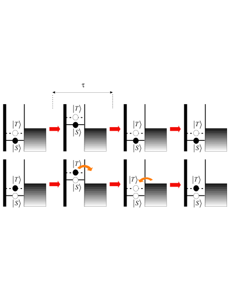
Figure 1: Schematic of the quantum dot throughout the non-destructive measurement scheme, for a singlet (Top) or triplet (Bottom) initial state. Curved arrows indicate tunnel process. The spin state is the same before and after the measurement.

To implement the non-destructive measurement, we pulse the potential of the dot so the electrochemical potential for both the singlet and the triplet state lies above the Fermi energy for a short time $\tau$ (see Fig. 1), fulfilling the relation $1/\Gamma_{T}\ll\tau\ll 1/\Gamma_{S}$. In the experiment, $1/\Gamma_{T}\approx 5~{}\mu s$, $\tau=20~{}\mu s$, and $1/\Gamma_{S,out}=100~{}\mu s$ (for the singlet, we observe the time to tunnel in is different from the time to tunnel out: $1/\Gamma_{S,in}\approx 1000~{}\mu s$ note3 ). If the dot is in the singlet state, most of the time no electron tunnels out during the entire pulse sequence since $\tau$ is small in comparison with $1/\Gamma_{S}$, even though tunneling would be energetically allowed. In the case of the triplet state, an electron will tunnel off the dot after the pulse is applied, in a time $1/\Gamma_{T}$ much smaller than $\tau$. In this case, an electron tunnels back in after the pulse and, it will tunnel into the triplet state with high probability since $\Gamma_{T}\gg\Gamma_{S}$.

The proposed read-out scheme is thus non-destructive in the sense that the state after the measurement coincides with the measurement result. The actual measurement takes place through the occurrence or absence of the first tunnel process. For a superposition input state, this is when the ”projection” of the wave function would take place. For a singlet initial state, the dot remains in the singlet all along; for a triplet initial state, the dot is reinitialized through a second tunnel event.

We point out that the proposed scheme is conceptually similar to the measurement procedure used for trapped ions WinelandRMP . In both systems, we can distinguish the two relevant states depending on whether or not a transition is made through a third state (a reservoir for the electron spin and a short-lived internal level for the ion).

We test this measurement concept with a quantum dot (white dotted circle in Fig. 2(a)) and a quantum point contact (QPC) defined in a two-dimensional electron gas (2DEG) with an electron density of $1.3\cdot 10^{15}$ m^-2, 90 nm below the surface of a GaAs/AlGaAs heterostructure, by applying negative voltages to gates $L$, $M$, $T$ and $Q$. Fast voltage pulses on gate $P$ are used to rapidly change the electrochemical potential of the dot. All measurements are performed at zero magnetic field. We tune the dot to the few-electron regime CiorgaPRB ; JeroFewEl , and completely pinch off the tunnel barrier between gates $L$ and $T$, so that the dot is only coupled to the reservoir on the right JeroAPL . The conductance of the QPC is tuned to about $e^{2}/h$, making it very sensitive to the number of electrons on the dot FieldPRL . A voltage bias of 0.7 mV induces a current through the QPC, $I_{QPC}$, of about 30 nA. Tunneling of an electron on or off the dot gives steps in $I_{QPC}$ of 300 pA LievenAPL ; EnsslinAPL and we observe them in the experiment with a measurement bandwidth equal to 60 kHz.

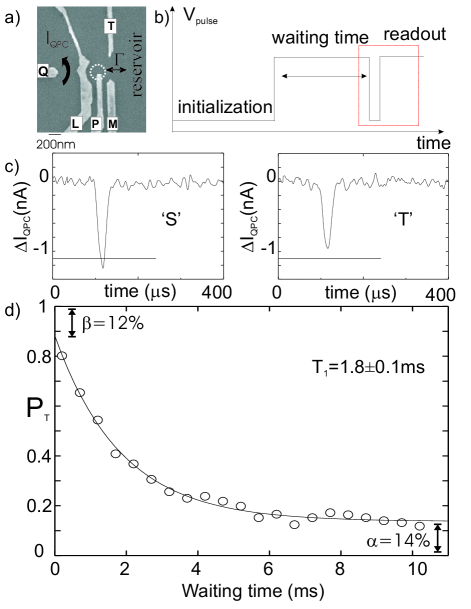
Figure 2: (a) Scanning electron micrograph showing the sample design. (b) Voltage pulses applied to gate ${}^{\prime}P^{\prime}$ for the relaxation measurement. (c) Typical QPC response in a 400 $\mu$s interval around the read-out pulse, for the case of singlet (left) and triplet (right). The solid horizontal line indicates the position of the threshold. (d) The probability for detecting a triplet state as a function of the waiting time. Each point is an average over $500$ experiments. The solid line is an exponential fit to the data. The measurement errors $\alpha$ and $\beta$ (see text) are indicated.

First we demonstrate that the non-destructive measurement correctly reads out the spin states. The experiment consists in reconstructing a relaxation curve from the triplet to the singlet and comparing the results with those obtained using destructive read-out scheme RonaldPRL . The protocol is illustrated in Fig.2(b). The starting point is a dot with one electron in the ground state (initialization). In the second stage of the pulse, the singlet and triplet electrochemical potentials are below the Fermi energy and a second electron tunnels into the dot. Since $\Gamma_{T}\gg\Gamma_{S}$, most likely a triplet state will be formed, on a timescale of $1/\Gamma_{T}$. The non-destructive measurement pulse is applied after a waiting time that we vary. Due to the direct capacitive coupling of gate $P$ to the QPC channel, $\Delta I_{QPC}$ follows the pulse shape (see Fig 2(c)). The precise amplitude of the QPC pulse response directly reflects the charge state of the dot throughout the read-out pulse. If the two electrons remain in the dot, the QPC signal goes below a predefined threshold, and we conclude that the dot was in the singlet state (outcome ${}^{\prime}S^{\prime}$, see Fig. 2(c), left). Otherwise, if one electron tunnels out in a time shorter than the pulse response time, the QPC pulse response stays above the threshold and we declare that the dot was in the triplet state (outcome ${}^{\prime}T^{\prime}$, see Fig. 2(c), right) sigma .

As expected, we observe an exponential decay of the triplet population as a function of the waiting time, giving a relaxation time, $T_{1}$, equal to $1.8\pm 0.1$ ms. The measurement errors are $\alpha=0.14$ and $\beta=0.12$, where $\alpha$ ($\beta$) is defined as the probability for the measurement to return triplet (singlet) if the actual state is singlet (triplet). We observe the same values (within error bars) when using the known destructive read-out scheme in this same measurement run. In both cases, measurement errors are completely explained by the two different tunnel rates RonaldPRL . The resulting measurement fidelity, $1-(\alpha+\beta)/2$, is 87%. It is worth noticing that in this new read-out scheme the measurement time, $t_{meas}\simeq\tau=20~{}\mu$s, is much shorter than $T_{1}$ ($T_{1}/t_{meas}\simeq 90$).

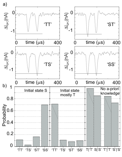
Figure 3: (a) Typical QPC response for two consecutive measurements in the case of ${}^{\prime}SS^{\prime}$, ${}^{\prime}TT^{\prime}$, ${}^{\prime}ST^{\prime}$ and ${}^{\prime}TS^{\prime}$. The threshold is the same for the two non-destructive measurement pulses. The pulse width is $20~{}\mu$s and the delay between the two measurement pulses is $60~{}\mu$s. (b) The recorded probabilities for each of these four events over 3000 runs, with the singlet (first graph) and mostly the triplet (second graph) as the initial state. In the third graph, conditional probabilities $P(T|^{\prime}T^{\prime})$ or $P(S|^{\prime}S^{\prime})$ that the state after the first measurement corresponds to the outcome of the first measurement and conditional probabilities $P(^{\prime}T^{\prime}|^{\prime}T^{\prime})$ or $P(^{\prime}S^{\prime}|^{\prime}S^{\prime})$ that the second measurement gives the same outcome as the first one are presented. They are extracted from the two previous graphs and the known $\alpha$ and $\beta$ with no a-priori knowledge of the initial state.

We next test if the measurement is non-destructive by studying the correlations between the outcomes of two successive measurements. We program a second read-out pulse $60~{}\mu$s after the end of the first pulse and record the probability for each of the four combined outcomes, ${}^{\prime}SS^{\prime}$, ${}^{\prime}TT^{\prime}$, ${}^{\prime}ST^{\prime}$, ${}^{\prime}TS^{\prime}$ (Fig.3). In order to accurately characterize the measurement, we first do this with singlet initial states (prepared by waiting $20$ ms for complete relaxation), and then again with mostly triplet initial states (prepared by letting the second electron tunnel in $200~{}\mu$s before the first measurement note1 ). A clear correlation between consecutive measurement outcomes is observed (Fig. 3(b)), both for singlet and triplet initial states.

When we average over $S$ or $T$ initial states (i.e. when we have no a-priori knowledge of the spin state), we find, from the correlation data and the known values of $\alpha$ and $\beta$, an $85\%$ ($73\%$) conditional probability for outcome ${}^{\prime}T^{\prime}$ (${}^{\prime}S^{\prime}$) in the second measurement given that the first measurement outcome was ${}^{\prime}T^{\prime}$ (${}^{\prime}S^{\prime}$) note2 .

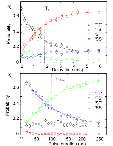
Figure 4: The probabilities for the two consecutive measurement outcomes as a function of (a) the measurement delay and (b) the measurement pulse duration. In solid line is represented the exponential fit to the data.

The degree to which the scheme is non-destructive is quantified via the probability for obtaining a $S$ or $T$ post measurement state ($60~{}\mu$s after the end of the first pulse) conditional on the measurement outcome. From the correlation data and the known values of $\alpha$ and $\beta$, we extract a $97\%$ ($84\%$) conditional probability $P(T|^{\prime}T^{\prime})$ ($P(S|^{\prime}S^{\prime}))$, again assuming no a-priori knowledge of the initial state note2 . For a triplet outcome, one electron tunneled out during the measurement pulse, and another electron tunneled back in after the pulse. A triplet state is formed with near certainty in this reinitialization process (since $\Gamma_{T}/\Gamma_{S,in}\approx 200$), but the triplet state can relax to the singlet during the $60~{}\mu$s wait time between the two measurements. This occurs with a probability $\gamma$ of $3\%$, which explains the observed conditional probability $P(T|^{\prime}T^{\prime})$. The conditional probability $P(S|^{\prime}S^{\prime})$ can be found as $1-P(T,^{\prime}S^{\prime})/P(^{\prime}S^{\prime})$. $P(^{\prime}S^{\prime})$ is simply $[(1-\alpha)+\beta]/2$ (averaged over $S$ and $T$ initial states). There are two main contributions to $P(T,^{\prime}S^{\prime})$. First, for $\beta=12\%$ of the triplet initial states, both electrons remain on the dot. In this case, a singlet outcome is declared but the post-measurement state is almost always a triplet. Second, for singlet initial states, a singlet outcome is obtained with probability $1-\alpha=86\%$. For $\sigma=5\%$ of those cases, one electron nevertheless tunneled out and the post-measurement state is a triplet note2 .

An attractive feature of non-destructive measurements is that it allows one to study the time evolution between two successive measurements. As a proof of principle, we let the spin evolve under relaxation for a controlled time in between two measurements. The singlet state is not affected by relaxation, so we initialize the dot (mostly, as before) in the triplet state. In figure 4(a), the probabilities for the four possible outcomes are recorded as a function of the waiting time. We notice that ${}^{\prime}TT^{\prime}$ and ${}^{\prime}TS^{\prime}$ respectively decay and increase exponentially, with a time constant $1.5\pm 0.3$ ms, within the error bars of the relaxation time obtained from Fig.2(d).

Finally, we remark that the non-destructive nature of the measurement relies on our ability to tune the dot in a regime where $1/\Gamma_{T}\ll\tau\ll 1/\Gamma_{S,out}$. If $\tau\gg 1/\Gamma_{S,out},1/\Gamma_{T}$, the measurement is destructive, because one electron will tunnel off the dot during the read-out pulse irrespective of the state of the dot. The information about the spin state is then lost after the read-out and the post-measurement state will always be a triplet. We can vary the duration of the pulse in order to make the transition from non-destructive to destructive read-out. Here we initialize in the singlet state, since for triplet initial states, the post-measurement state doesn’t change with $\tau$. Figure 4(b) summarizes the results. The four different curves correspond to each combination of measurement outcomes as a function of the duration of the pulse. As expected, the ${}^{\prime}TS^{\prime}$ and ${}^{\prime}TT^{\prime}$ statistics are steady, while the ${}^{\prime}SS^{\prime}$ and ${}^{\prime}ST^{\prime}$ probabilities decay respectively increase exponentially with a time constant $105\pm 10~{}\mu s$, within the error bars of the evaluation of $1/\Gamma_{S,out}$.

In conclusion, we demonstrate our ability to implement a non-destructive measurement scheme for distinguishing two-electron singlet from triplet states in a single quantum dot. The spin system is not strictly preserved throughout the entire measurement process. In that respect, our scheme differs from a quantum non-demolition (QND) measurement Braginsky . Nevertheless, repeated measurements give the same results and the post-measurement state corresponds to the measurement outcome. All the imperfections in the correlations observed in the experiments are explained by the ratio between the singlet and triplet tunnel rates, and the relaxation rate from triplet to singlet. Other spin-dependent tunnel processes, for instance as observed in double dots EngelPRL04 ; KoppensScience ; JohnsonNature ; PettaScience , can be used for non-destructive read-out, possibly with even higher fidelity.

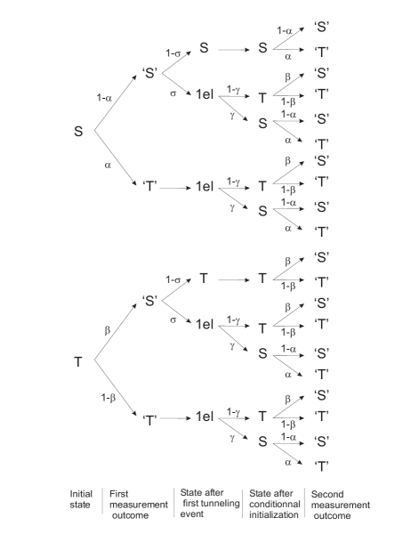
Figure 5: Different events and their probabilities all along the process of the two consecutive measurements for singlet S or triplet T as an initial state. $\alpha$ and $\beta$ are defined as the probability for the measurement to return respectively triplet and singlet if the actual state is singlet and triplet. They are obtained directly from the relaxation curve, giving $\alpha=14\%$ and $\beta=12\%$. $\sigma$ is the probability for an electron to tunnel out even though the QPC signal did go below the threshold and a ${}^{\prime}S^{\prime}$ outcome has been declared (we assume that $\sigma$ is equal for singlet and triplet initial states). Finally, $\gamma$ is the probability that, after reinitializing to a two-electron state and subsequent relaxation for $60~{}\mu$s, a singlet state is present in the dot. In the experiment, $\sigma=5\%$ and $\gamma=3\%$, determined from the above probability tree, the known value of $\alpha$ and $\beta$, and the correlation data.

- (1) V. B. Braginsky and F. Y. Khalili, Quantum measurement, Camb. Univ. Press (1995).
- (2) D.P. DiVincenzo, Forschr. Phys. 48, 771 (2000).
- (3) M. Field et al., Phys. Rev. Lett. 70, 1311 (1993).
- (4) J. R. Petta et al., Phys. Rev. Lett. 93, 186802 (2004).
- (5) J. M. Elzerman et al., Nature 430, 431 (2004).
- (6) R. Hanson et al., Phys. Rev. Lett. 94, 196802 (2005).
- (7) Miro Kroutvar et al., Nature 432, 81 (2001).
- (8) A possible explanation could be that the pulse not only shifts the dot potential but also distorts it, thereby changing the orbitals.
- (9) D. Leibfried, R. Blatt, C. Monroe, and D. Wineland, Rev. Mod. Phys. 75, 281 (2003).
- (10) M. Ciorga et al., Phys. Rev. B 61, R16315 (2000)
- (11) J. M. Elzerman et al., Phys. Rev. B 67, 161308 (2003).
- (12) J. M. Elzerman et al., Appl. Phys. Lett. 84, 4617 (2004).
- (13) R. Schleser et al., Appl. Phys. Lett. 85, 2005 (2004).
- (14) L. M. K. Vandersypen et al., Appl. Phys. Lett. 85, 4394 (2004).
- (15) When the QPC signal went below the threshold and a outcome is declared, there is still some probability, , that one electron tunneled out during the pulse (after a time longer than the pulse response time).
- (16) The ratio of and tunnel rates into the dot is , but of the triplets relax to singlet in the short time between injection and read-out (s).
- (17) Full details of the statistics of all processes are available as supplementary material.
- (18) Hans-Andreas Engel et al., Phys. Rev. Lett. 93, 106804 (2004).
- (19) A. C. Johnson et al., Nature 435, 925 (2005).
- (20) F. H. L. Koppens et al., Science 309, 1346 (2005).
- (21) J. R. Petta et al., Science 309, 2180 (2005).